Parameter Estimation and Hypothesis Testing of Multivariate Poisson Inverse Gaussian Regression


Abstract
1. Introduction
2. Materials and Methods
2.1. Multivariate Poisson Inverse Gaussian Distribution (MPIGD)
2.2. Multivariate Poisson Inverse Gaussian Regression (MPIGR)
3. Results
3.1. Parameter Estimation of MPIGR Model
- ▪
- Step 1. Determine the initial value for parameter . The initial value of parameter is obtained while using the separate univariate Poisson regression. The initial value for overdispersion parameter τ used the average of the observed overdispersion based on the variance of PIGD [9].
- ▪
- Step 2. Determine the gradient vector , which is the elements consist of the first derivative of the log-likelihood function, .
- ▪
- Step 3. Determine the Hessian matrix where the elements consist of the second derivative of the log-likelihood function, as follows
- ▪
- Step 4. Start the Newton–Raphson iteration using the following formula,with and r = 0, 1, 2, …, r*.
- ▪
- Step 5. The iteration will stop if , with ε is a very small value and it will produce the estimator value for each parameter.
3.2. Factorial Simplification in the Third Modification of BESSEL Function
3.3. Hypothesis Testing of MPIGR Model
3.4. Application
4. Discussion
5. Conclusions
Author Contributions
Funding
Acknowledgments
Conflicts of Interest
Nomenclature
| PIG | Poisson Inverse Gaussian |
| PIGD | Poisson Inverse Gaussian Distribution |
| PIGR | Poisson Inverse Gaussian Regression |
| MPIGD | Multivariate Poisson Inverse Gaussian Distribution |
| MPIGR | Multivariate Poisson Inverse Gaussian Regression |
| MLE | Maximum Likelihood Function |
| MLRT | Maximum Likelihood Ratio Test |
| CoV | Coefficient of Variation |
| LBW | Low Birth Weight |
Appendix A
References
- Consul, P.; Famoye, F. Generalized poisson regression model. Commun. Stat. Theory Methods 1992, 21, 89–109. [Google Scholar] [CrossRef]
- Holla, M.S. On a poisson-inverse gaussian distribution. Metr. Int. J. Theor. Appl. Stat. 1967, 11, 115–121. [Google Scholar] [CrossRef]
- Dean, C.; Lawless, J.F.; Willmot, G.E. A mixed poisson-inverse-gaussian regression model. Can. J. Stat. 1989, 17, 171–181. [Google Scholar] [CrossRef]
- Hilbe, J.M. Poisson Inverse Gaussian Regression. In Modeling Count Data; Cambridge University Press (CUP): Cambridge, UK, 2014; pp. 162–171. [Google Scholar]
- Karlis, D.; Xekalaki, E. A Simulation Comparison of Several Procedures for Testing the Poisson Assumption. J. R. Stat. Soc. Ser. D Stat. 2000, 49, 355–382. [Google Scholar] [CrossRef][Green Version]
- Ouma, V.M. Poisson Inverse Gaussian (PIG) Model for Infectious Disease Count Data. Am. J. Theor. Appl. Stat. 2016, 5, 326. [Google Scholar] [CrossRef][Green Version]
- Xie, F.-C.; Wei, B.-C. Influence analysis for Poisson inverse Gaussian regression models based on the EM algorithm. Metrika 2007, 67, 49–62. [Google Scholar] [CrossRef]
- Zha, L.; Lord, D.; Zou, Y. The Poisson inverse Gaussian (PIG) generalized linear regression model for analyzing motor vehicle crash data. J. Transp. Saf. Secur. 2014, 8, 18–35. [Google Scholar] [CrossRef]
- Ghitany, M.E.; Karlis, D. An EM Algorithm for Multivariate Mixed Poisson. Appl. Math. Sci. 2012, 6, 6843–6856. [Google Scholar]
- United Nations Inter-agency Group for Child Mortality Estimation (UN IGME). Levels & Trends in Child Mortality: Report 2018, Estimates Developed by the United Nations Inter-Agency Group for Child Mortality Estimation; United Nations Children’s Fund: New York, NY, USA, 2018. [Google Scholar]
- WHO; UNICEF; UNFPA; The World Bank. Maternal Mortality: Level and Trends 2000 to 2017; World Health Organization: Geneva, Switzerland, 2019; ISBN 978-92-4-151648-8. [Google Scholar]
- Moucheraud, C.; Worku, A.; Molla, M.; Finlay, J.E.; Leaning, J.; Yamin, A.E. Consequences of maternal mortality on infant and child survival: A 25-year longitudinal analysis in Butajira Ethiopia (1987–2011). Reprod. Health 2015, 12, S4. [Google Scholar] [CrossRef] [PubMed]
- Miaou, S.P.; Lord, D. Modeling Traffic Crash–Flow Relationships for Intersections Dispersion Parameter, Functional Form, and Bayes Versus Empirical Bayes Methods. Transp. Res. Rec. J. Transp. Res. Board 2003, 1840, 31–40. [Google Scholar] [CrossRef]
- Willmot, G.E. The Poisson-Inverse Gaussian distribution as an alternative to the negative binomial. Scand. Actuar. J. 1987, 1987, 113–127. [Google Scholar] [CrossRef]
- Stein, G.Z.; Juritz, J.M. Bivariate compound poisson distributions. Commun. Stat. Theory Methods 1987, 16, 3591–3607. [Google Scholar] [CrossRef]
- Stein, G.Z.; Zucchini, W.; Juritz, J.M. Parameter estimation for the Sichel distribution and its multivariate extension. J. Am. Stat. Assoc. 1987, 82, 938–944. [Google Scholar] [CrossRef]


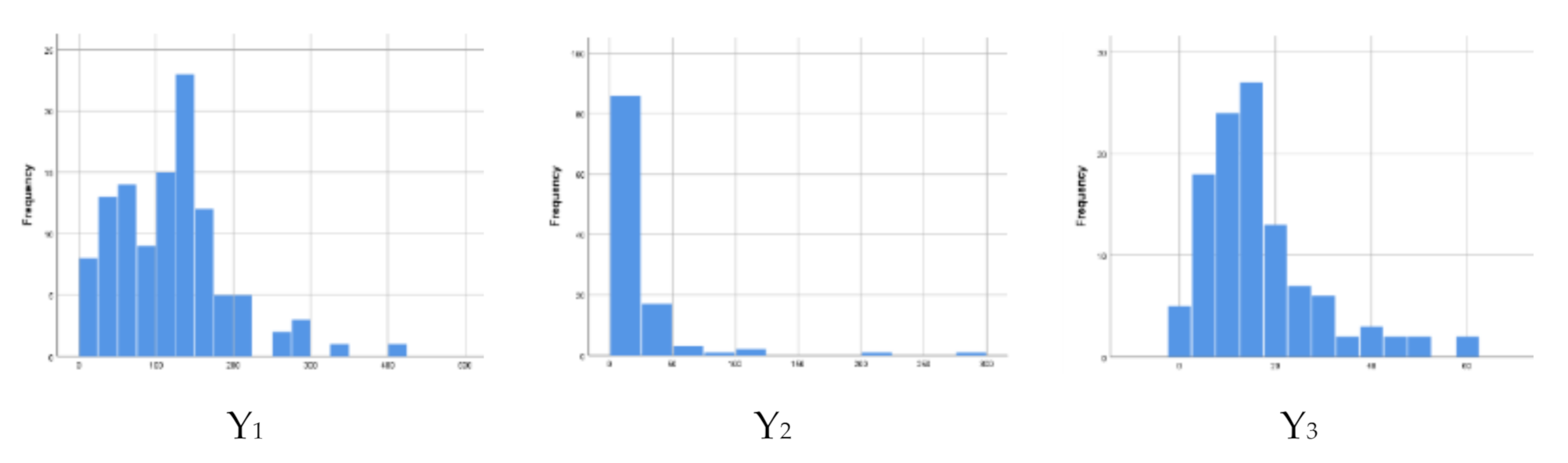
| Variable | Mean | SD | Coefficient of Variation | Min | Max |
|---|---|---|---|---|---|
| The number of infant mortality (Y1) | 118.08 | 72.885 | 63.4 | 7 | 403 |
| The number of child mortality (Y2) | 20.41 | 36.554 | 425.6 | 0 | 278 |
| The number of maternal mortality (Y3) | 16.4 | 12.233 | 89.1 | 0 | 59 |
| Variable | Province | ||||
|---|---|---|---|---|---|
| Jakarta | Yogyakarta | Central Java | West Java | East Java | |
| The percentage of antenatal care visit by pregnant women | 99.26 (6.10) a | 90.92 (3.61) | 92.86 (3.62) | 97.44 (8.20) | 89.34 (5.47) |
| The percentage of pregnant woman who received Fe3 tablet | 95.14 (4.35) | 88.05 (4.41) | 92.85 (4.01) | 95.88 (9.50) | 88.37 (5.67) |
| The percentage of complete neonatal visits | 95.44 (2.13) | 77.32 (28.53) | 92.97 (10.29) | 94.30 (16.78) | 96.34 (3.82) |
| The percentage of Low Birth Weight (LBW) | 1.07 (1.45) | 5.26 (1.14) | 4.54 (0.93) | 2.87 (1.66) | 4.20 (1.41) |
| The percentage of healthy house | 66.33 (18.85) | 70.59 (17.97) | 85.27 (14.17) | 71.25 (15.84) | 70.53 (16.40) |
| The percentage of active integrated service post | 100 (0.00) | 76.99 (9.36) | 66.98 (18.88) | 63.07 (20.58) | 78.14 (14.53) |
| The percentage of infants received vitamin A | 92.52 (8.13) | 90.92 (16.40) | 97.25 (8.43) | 91.76 (16.01) | 98.30 (7.97) |
| The percentage of births assisted by health workers | 98.00 (5.56) | 100.0 (0.00) | 99.14 (1.56) | 97.94 (8.39) | 94.04 (4.16) |
| The number of live births b | 34649 (23137) | 8470 (4548) | 15424 (7310) | 33903 (25870) | 15144 (10125) |
| Variable | Deviance | df | Deviance/df |
|---|---|---|---|
| Number of infant mortality (Y1) | 4462.60 | 102 | 43.75 |
| Number of child mortality (Y2) | 2181.11 | 102 | 21.38 |
| Number of maternal mortality (Y3) | 670.05 | 102 | 6.57 |
| Parameter | The Number of Infant Mortality | The Number of Under-Five Children Mortality | The Number of Maternal Mortality | |||||||||
|---|---|---|---|---|---|---|---|---|---|---|---|---|
| Est | Se | Z | P | Est | Se | Z | P | Est | Se | Z | P | |
| 4.101 | 5.27 × 10⁻⁴ | −7.78 × 10³ | p < 0.001 | −2.549 | 5.17 × 10⁻³ | 4.92 × 10² | p < 0.001 | 3.613 | 3.59 × 10⁻² | −1.00 × 10² | p < 0.001 | |
| −0.032 | 7.40 × 10⁻⁸ | 4.31 × 10⁵ | p < 0.001 | −0.072 | 7.24 × 10⁻⁷ | 9.89 × 10⁴ | p < 0.001 | 0.014 | 1.06 × 10⁻⁵ | −1.34 × 10³ | p < 0.001 | |
| 0.004 | 6.23 × 10⁻⁸ | 6.16 × 10⁴ | p < 0.001 | −0.018 | 6.15 × 10⁻⁷ | −2.87 × 10⁴ | p < 0.001 | 0.007 | 3.05 × 10⁻⁶ | 2.31 × 10³ | p < 0.001 | |
| −0.003 | 5.16 × 10⁻⁹ | −5.33 × 10⁵ | p < 0.001 | 0.001 | 5.03 × 10⁻⁹ | −2.64 × 10⁵ | p < 0.001 | −0.003 | 4.43 × 10⁻⁸ | −6.09 × 10⁴ | p < 0.001 | |
| −0.076 | 6.83 × 10⁻⁷ | 1.11 × 10⁵ | p < 0.001 | −0.449 | 1.41 × 10⁻⁵ | 3.18 × 10⁴ | p < 0.001 | −0.119 | 3.54 × 10⁻⁵ | 3.36 × 10³ | p < 0.001 | |
| −0.002 | 3.88 × 10⁻⁹ | 4.88 × 10⁵ | p < 0.001 | 0.005 | 2.04 × 10⁻⁸ | 2.24 × 10⁵ | p < 0.001 | −0.005 | 3.99 × 10⁻⁷ | 1.28 × 10⁴ | p < 0.001 | |
| −0.005 | 3.67 × 10⁻⁹ | 1.37 × 10⁶ | p < 0.001 | 0.019 | 2.53 × 10⁻⁸ | −7.59 × 10⁵ | p < 0.001 | −0.013 | 2.60 × 10⁻⁷ | 5.34 × 10⁴ | p < 0.001 | |
| 0.004 | 6.67 × 10⁻⁹ | −6.03 × 10⁵ | p < 0.001 | −0.005 | 2.02 × 10⁻⁸ | −2.57 × 10⁵ | p < 0.001 | 0.006 | 8.32 × 10⁻⁷ | −7.68 × 10³ | p < 0.001 | |
| 0.041 | 3.26 × 10⁻⁸ | 1.24 × 10⁶ | p < 0.001 | 0.144 | 1.94 × 10⁻⁶ | 7.42 × 10⁴ | p < 0.001 | 3.613 | 3.59 × 10⁻² | −1.00 × 10² | p < 0.001 | |
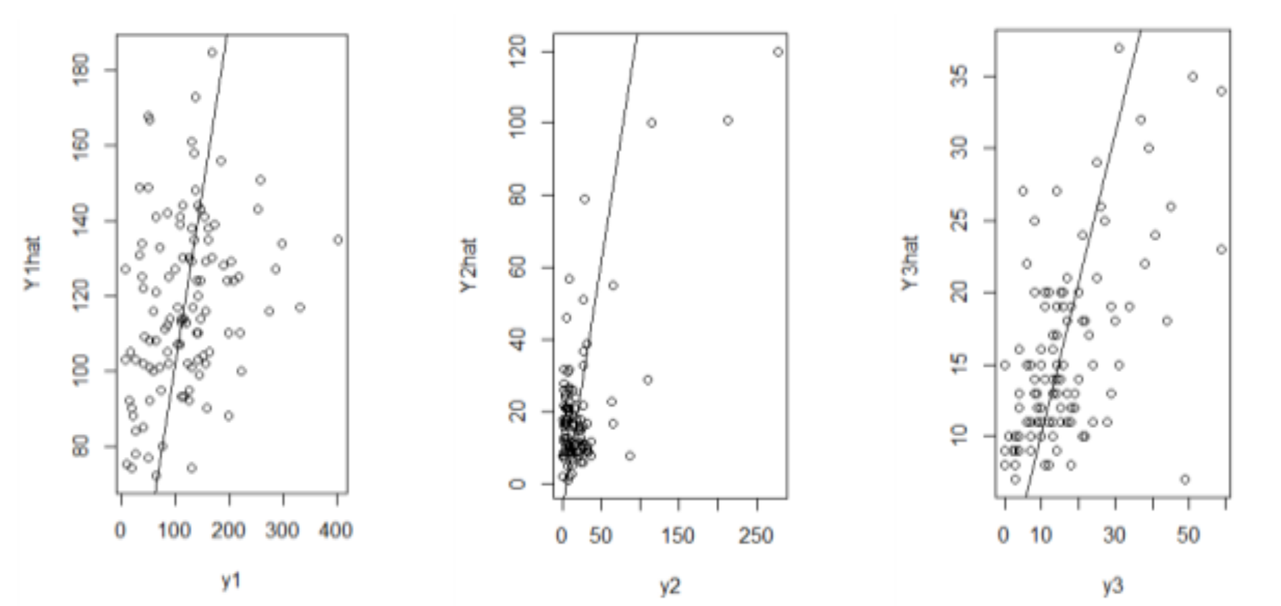
| Y1 | Y2 | Y3 | |
|---|---|---|---|
| MSE | 4821.05 | 707.31 | 104.17 |
| RMSE | 69.43 | 26.59 | 10.21 |
Publisher’s Note: MDPI stays neutral with regard to jurisdictional claims in published maps and institutional affiliations. |
© 2020 by the authors. Licensee MDPI, Basel, Switzerland. This article is an open access article distributed under the terms and conditions of the Creative Commons Attribution (CC BY) license (http://creativecommons.org/licenses/by/4.0/).
Share and Cite
Mardalena, S.; Purhadi, P.; Purnomo, J.D.T.; Prastyo, D.D. Parameter Estimation and Hypothesis Testing of Multivariate Poisson Inverse Gaussian Regression. Symmetry 2020, 12, 1738. https://doi.org/10.3390/sym12101738
Mardalena S, Purhadi P, Purnomo JDT, Prastyo DD. Parameter Estimation and Hypothesis Testing of Multivariate Poisson Inverse Gaussian Regression. Symmetry. 2020; 12(10):1738. https://doi.org/10.3390/sym12101738
Chicago/Turabian StyleMardalena, Selvi, Purhadi Purhadi, Jerry Dwi Trijoyo Purnomo, and Dedy Dwi Prastyo. 2020. "Parameter Estimation and Hypothesis Testing of Multivariate Poisson Inverse Gaussian Regression" Symmetry 12, no. 10: 1738. https://doi.org/10.3390/sym12101738
APA StyleMardalena, S., Purhadi, P., Purnomo, J. D. T., & Prastyo, D. D. (2020). Parameter Estimation and Hypothesis Testing of Multivariate Poisson Inverse Gaussian Regression. Symmetry, 12(10), 1738. https://doi.org/10.3390/sym12101738