On Construction of Solutions of Linear Differential Systems with Argument Deviations of Mixed Type

Abstract

We show the use of parametrization techniques and successive approximations for the effective construction of solutions of linear boundary value problems for differential systems with multiple argument deviations. The approach is illustrated with a numerical example.

1. Introduction

In several applications, it is desirable to have effective tools allowing one to construct solutions of functional differential equations under various boundary conditions. Many real processes are modelled by systems of equations with argument deviations (see, e.g., [1,2,3] and references therein). For delay equations, the classical method of steps [1] allows one to construct the solution of the Cauchy problem by extending it from the initial interval in a stepwise manner; in this way, an ordinary differential equation is solved at every step, with every preceding part of the curve serving as a historical function for the next one. This technique, together with the ODE solvers available in the mathematical software, is commonly used in the practical analysis of dynamic models based on equations with retarded argument under the initial conditions (e.g., in economical models [4,5,6]).

In certain cases, boundary conditions are more complicated and deviations are of mixed type (i. e., equations involve both retarded and advanced terms [7,8] or deviations of neither type), which in particular, makes impossible to apply the method of steps due to the absence of the Volterra property of the corresponding operator. The aim of this paper is to show that the techniques suggested in [9] for boundary value problems for ordinary differential equations, under certain assumptions, can be adopted for application to functional differential equations covering, in particular, the case of deviations of mixed type and general boundary conditions. As a result, one can formulate a scheme for the effective finding of approximations to solutions of boundary value problems for functional differential equations, which also theoretically allows one to establish the solvability in a rigorous manner. Here, we consider the linear case and deal with the construction of approximate solutions only. The techniques are rather flexible and can be used in relation to other problems. Although the approach is not explicitly designed for partial differential equations, it still might be used in the cases where systems of equations with one independent variable arise (e.g., equations obtained when a symmetry reduction is possible, equations related to the inverse scattering transform or discretization [10,11]). Unlike methods used for integrable systems (e.g., the Hirota bilinear method [12]), the technique is aimed at getting approximate solutons without previous knowledge of the structure of the solution set.

We consider the system of n linear functional differential equations

$$u^{\prime }(t)=(lu)(t)+q(t),t\in [a,b],$$

(1)

under the linear boundary conditions

$$h(u)=d,$$

(2)

where $u={(u_i)}_{i=1}^n$, $-\infty <a<b<\infty$, $l:C([a,b],{\mathbb{R}}^n)\to L_{\infty }([a,b],{\mathbb{R}}^n)$ is a linear bounded operator, $h:C([a,b],{\mathbb{R}}^n)\to {\mathbb{R}}^n$ is a bounded linear vector-valued functional, $d=\mathrm{col}\left(d_1,\cdots ,d_n\right)$ and $q\in L_{\infty }([a,b],{\mathbb{R}}^n)$ are fixed. System (1) can be rewritten in coordinates as

$$\begin{array}{cc}\hfill u_i^{\prime }(t)& =\sum _{j=1}^n(l_{ij}u)(t)+q_i(t),t\in \left[a,b\right],i=1,\cdots ,n,\hfill \end{array}$$

(3)

where $l_{ij}:C([a,b],\mathbb{R})\to L_{\infty }([a,b],\mathbb{R})$ are the components of the operator $l=\mathrm{col}(l_1,\cdots ,l_n)$ defined by the equalities

$$l_{ij}v:=l_i(v{e}_j),i,j=1,2,\cdots ,n$$

(4)

for v from $C([a,b],\mathbb{R})$ (here, $e_j$ stands for the jth unit vector). The difference between (1) and (3) is a matter of notation: given system (3), it can be rewritten as (1) by setting

$$lu=\left(\begin{array}{c}{\displaystyle \sum _{j=1}^n{l}_{1j}(u_j)}\\ {\displaystyle \sum _{j=1}^n{l}_{2j}(u_j)}\\ \cdots \\ {\displaystyle \sum _{j=1}^n{l}_{nj}(u_j)}\end{array}\right)$$

(5)

for $u\in C([a,b],{\mathbb{R}}^n)$. Here, we consider the case where the component operators have values in $L_{\infty }([a,b],\mathbb{R})$, i. e., the coefficients in the equation are essentially bounded, which excludes the presence of integrable singularities (e.g., $1/\sqrt{t}$, $t\in (0,1]$).

System (3) covers, in particular, the system of differential equations with argument deviations of the form

$$u_i^{\prime }(t)=\sum _{j=1}^n{p}_{ij}(t)u_j({\tau }_{ij}(t))+q_i(t),t\in \left[a,b\right],i=1,\cdots ,n,$$

(6)

where ${\tau }_{ij}:[a,b]\to [a,b]$, are measurable functions, $p_{ij}:\left[a,b\right]\to \mathbb{R}$ and $q_i:[a,b]\to \mathbb{R}$ $i,j=1,\cdots ,n$, are from $L_{\infty }([a,b],\mathbb{R})$. A particular case of (6) is, e.g., the well-known pantograph equation, which arises independently in several applied problems of various nature (see, e.g., [13,14] and references therein). The assumption that ${\bigcup }_{i,j=1}^n{\tau }_{ij}([a,b])\subset [a,b]$ is not a restriction of generality because the setting involving initial functions can be reduced to the present one by a suitable transformation [15]. The retarded character of the equation is not assumed (in particular, for (6), it is not required that ${\tau }_{ij}(t)\le t$ for all i, j) and, therefore, the method of steps is inapplicable.

We use the following notation. For any vectors $\xi =\mathrm{col}({\xi }_1,\cdots ,{\xi }_n)$, $\eta =\mathrm{col}({\eta }_1,\cdots ,{\eta }_n)$, we write $\left|\xi \right|=\mathrm{col}(\left|{\xi }_1\right|,\cdots ,\left|{\xi }_n\right|)$ and

$$max\{\xi ,\eta \}=\mathrm{col}(max\{{\xi }_1,{\eta }_1\},\cdots ,max\{{\xi }_n,{\eta }_n\}).$$

(7)

The inequalities between vectors as well as minima and maxima of vector functions are understood likewise in the componentwise sense. $r(A)$ denotes the spectral radius of a matrix A. For an essentially bounded function $v:[a,b]\to {\mathbb{R}}^n$ and an interval $J\subseteq [a,b]$, we put

$${\delta }_J(v):=\underset{t\in J}{\mathrm{ess}\sup }v(t)-\underset{t\in J}{\mathrm{ess}\inf }v(t).$$

(8)

2. Auxiliary Problems with Two-Point Conditions

The idea is to use a suitable parametrization. Motivated by [9], we will seek for a solution of (1), (2) among all solutions of Equation (1) under the simplest two-point conditions

$$\begin{array}{cccc}\hfill u(a)& =\xi ,\hfill & \hfill u(b)& =\eta \hfill \end{array}$$

(9)

with unfixed boundary values $\xi$ and $\eta$. Under suitable assumptions, every problem (1), (9) is shown to be uniquely solvable and its solution is constructed as the limit of certain iterations $\{u_m(·,\xi ,\eta ):m\ge 0\}$. The vectors $z=\mathrm{col}\left({\xi }_1,{\xi }_2,\cdots ,{\xi }_n\right)$ and $\eta =\mathrm{col}\left({\eta }_1,{\eta }_2,\cdots ,{\eta }_n\right)$ are parameters the values of which remain unknown at the moment; they should be chosen appropriately in order to satisfy condition (2).

Let us fix closed bounded connected sets $D_0$ and $D_1$ in ${\mathbb{R}}^n$ and focus on the solutions of problem (1), (2) with the values at the endpoints such that

$$\begin{array}{cccc}\hfill u(a)& \in D_0,\hfill & \hfill u(b)& \in D_1.\hfill \end{array}$$

(10)

To treat solutions with properties (10), we carry out “freezing” at the endpoints by passing temporarily to conditions (9). Thus, instead of (1), (2) we will consider the parametrised problem (1), (9). There are two (or, in coordinates, $2n$) degrees of freedom there and we will see that one can, in a sense, go back to the original problem by choosing the values of the parameters appropriately.

3. Iteration Process

Let $\mathcal{L}:L_{\infty }([a,b],{\mathbb{R}}^n)\to L_{\infty }([a,b],{\mathbb{R}}^n)$ be the continuous linear operator defined by the equality

$$(\mathcal{L}y)(t):={\int }_a^{t}y(s)ds-\frac{t-a}{b-a}{\int }_a^{b}y(s)ds,t\in [a,b],$$

(11)

for any $y\in L_{\infty }([a,b],{\mathbb{R}}^n)$. Let us fix arbitrary values of $\xi$ and $\eta$, put

$$\tilde{q}:=\mathcal{L}q,$$

(12)

and define the sequence of functions $\{u_m(·,\xi ,\eta ):m\ge 0\}$ by setting

$$\begin{array}{cc}\hfill u_0(t,\xi ,\eta )& =\left(1-\frac{t-a}{b-a}\right)\xi +\frac{t-a}{b-a}\eta ,\hfill \end{array}$$

(13)

$$\begin{array}{cc}\hfill u_m(t,\xi ,\eta )& =u_0(t,\xi ,\eta )+\tilde{q}(t)+(\mathcal{L}l{u}_{m-1}(·,\xi ,\eta ))(t),t\in [a,b],\hfill \end{array}$$

(14)

for $m\ge 1$. When no confusion may arise, for the sake of convenience we will sometimes omit the arguments $\xi$, $\eta$ in $u_m(t,\xi ,\eta )$ and write simply $u_m(t)$ assuming the dependence on the parameters implicitly. The sequence is obviously related to the iterative solution of the equation

$$u=u_0+\mathcal{L}lu+\tilde{q}.$$

(15)

The reason for choosing it in this particular way is explained by the following statement, which is an immediate consequence of (14).

Lemma 1.

Let ξ and η be fixed. If$u_m(·,\xi ,\eta )\rightrightarrows u$as$m\to +\infty$on$[a,b]$, then u satisfies the two-point conditions (9) and the equation

$$\begin{array}{cc}\hfill u^{\prime }(t)& =(lu)(t)+q(t)+\frac{1}{b-a}\left(\eta -\xi -{\int }_a^b(lu)(s)ds-{\int }_a^{b}q(s)ds\right),t\in [a,b].\hfill \end{array}$$

(16)

Proof. 

The function u satisfies the integral Equation (15) and, in particular, is absolutely continuous. By (11) and (13), Equation (15) is rewritten as

$$\begin{array}{cc}\hfill u(t)& =\xi +\frac{t-a}{b-a}(\eta -\xi )+{\int }_a^t(lu)(s)ds+{\int }_a^{t}q(s)ds-\frac{t-a}{b-a}\left({\int }_a^b(lu)(s)ds+{\int }_a^{b}q(s)ds\right),\hfill \end{array}$$

(17)

the differentiation of which yields (16). Since obviously $u_m(a,\xi ,\eta )=\xi$ and $u_m(b,\xi ,\eta )=\eta$ for all m, the fulfilment of conditions (9) is verified by passing to the limit in (14). □

The idea of the approach is briefly this: Equation (16) differs from (1) by a finite-dimensional term and after its ultimate “removal” by adjusting $\xi$ appropriately we are among the solutions of (1), (9); then we should try to choose $\eta$ so that (2) is satisfied. In order to proceed according to this scheme, it is needed to ensure the convergence of sequence of functions (14).

4. Applicability Conditions

Let L be the matrix constituted by the norms of the components of l as operators from $C([a,b],\mathbb{R})$ to $L_{\infty }([a,b],\mathbb{R})$:

$$L:=\left(\begin{array}{cccc}\parallel l_{11}\parallel & \parallel l_{12}\parallel & \cdots & \parallel l_{1n}\parallel \\ \parallel l_{21}\parallel & \parallel l_{22}\parallel & \cdots & \parallel l_{2n}\parallel \\ \cdots & \cdots & \cdots & \cdots \\ \parallel l_{n1}\parallel & \parallel l_{n2}\parallel & \cdots & \parallel l_{nn}\parallel \end{array}\right).$$

(18)

All the components of the matrix L are well defined due to the boundedness of l as a mapping from $C([a,b],{\mathbb{R}}^n)$ to $L_{\infty }([a,b],{\mathbb{R}}^n)$. It follows immediately from (4) and (18) that the componentwise inequality

$$\left|(lu)(t)\right|\le L\underset{s\in [a,b]}{max}\left|u(s)\right|$$

(19)

holds for a.e. $t\in [a,b]$ and arbitrary u from $C([a,b],{\mathbb{R}}^n)$.

Theorem 1.

Assume that the spectral radius of L satisfies the inequality

$$r(L)<\frac{2}{b-a}.$$

(20)

Then, for any fixed$\xi \in D_0$, $\eta \in D_1$, the sequence$\{u_m(·,\xi ,\eta ):m\ge 0\}$converges to a certain function$u_{\infty }(·,\xi ,\eta )$as$m\to +\infty$uniformly on$[a,b]$. The function$u_{\infty }(·,\xi ,\eta )$satisfies conditions (9) and the differential equation

$$\begin{array}{cc}\hfill u^{\prime }(t)& =(lu)(t)+q(t)+\frac{1}{b-a}\Delta (\xi ,\eta ),t\in [a,b],\hfill \end{array}$$

(21)

where

$$\Delta (\xi ,\eta ):=\eta -\xi -{\int }_a^b(l{u}_{\infty }(·,\xi ,\eta ))(s)ds-{\int }_a^{b}q(s)ds.$$

(22)

The function$u_{\infty }(·,\xi ,\eta )$is the unique solution of (21) with the initial condition$u(a)=\xi$and also the unique solution of Equation (17). The function$u_{\infty }(·,\xi ,\eta )$satisfies the original Equation (1) if and only if ξ and η are chosen so that

$$\Delta (\xi ,\eta )=0.$$

(23)

The form of iteration sequence (14) is chosen specifically according to the two-point separated boundary conditions (9), so that (9) is automatically satisfied on every step. The smallness of $r(L)$ (assumption (20)) ensures the unique solvability of all the auxiliary initial value problems (16) and (24),

$$u(a)=\xi ,$$

(24)

which is also helpful in cases where the initial value problem (1), (24) for the original equation is not uniquely solvable. It should be noted that the last mentioned issue may arise even for very simple equations of type (6); for example, it is easy to verify that if (1) has the form

$$u^{\prime }(t)=\frac{u(b)}{b-a}-q(t),t\in [a,b],$$

(25)

then the initial value problem (25), (24) is not uniquely solvable (it has infinitely many solutions if $\xi ={\int }_a^{b}q(s)ds$ and no solution for $\xi \ne {\int }_a^{b}q(s)ds$) and the corresponding Picard iterations diverge. However, the iterations defined according to equalities (13) and (14) can be used since assumption (20) is satisfied ($L={(b-a)}^{-1}$ in this case).

Equation (21) clearly resembles (16) with the difference that $\Delta (\xi ,\eta )$ appearing in (21), where the limit function is directly involved, is not a functional term. Equation (21) can thus be regarded as a perturbation of equation (1) with a constant forcing term,

$$\begin{array}{cc}\hfill u^{\prime }(t)& =(lu)(t)+q(t)+\mu ,t\in [a,b],\hfill \end{array}$$

(26)

the value of which is related to the two-point condition (9).

Theorem 2.

Assume that condition (20) holds and ξ, η are fixed. Then the solution of (26) with the initial value (24) satisfies the condition

$$u(b)=\eta$$

(27)

if and only if

$$\mu =\frac{1}{b-a}\Delta (\xi ,\eta )$$

(28)

with Δ given by (22).

Proof. 

The proof is similar to that of ([9] Theorem 7). If $\mu$ in (26) has form (28), then the function $u=u_{\infty }(·,\xi ,\eta )$, which is well defined by Theorem 1, is the unique solution of the Cauchy problem (26), (24). By Lemma 1, this function also satisfies condition (27).

Conversely, let v be a function satisfying (26) and (24) with a certain value of $\mu$. The integration of (26) gives the representation

$$\begin{array}{cc}\hfill v(t)& =\xi +{\int }_a^t(lv)(s)ds+{\int }_a^{t}q(s)ds+\mu \frac{t-a}{b-a},t\in [a,b],\hfill \end{array}$$

(29)

whence

$$\begin{array}{cc}\hfill (b-a)\mu & =v(b)-\xi -{\int }_a^b(lv)(s)ds-{\int }_a^{b}q(s)ds.\hfill \end{array}$$

(30)

Combining (29) and (30) and assuming that $v(b)=\eta$, we get

$$\begin{array}{cc}\hfill v(t)& =\xi +{\int }_a^t(lv)(s)ds+{\int }_a^{t}q(s)ds+\frac{t-a}{b-a}\left(\eta -\xi -{\int }_a^b(lv)(s)ds-{\int }_a^{b}q(s)ds\right),\hfill \end{array}$$

or, which is the same,

$$\begin{array}{cc}\hfill v(t)& =\xi +\frac{t-a}{b-a}(\eta -\xi )+{\int }_a^t(lv)(s)ds+{\int }_a^{t}q(s)ds-\frac{t-a}{b-a}\left({\int }_a^b(lv)(s)ds+{\int }_a^{b}q(s)ds\right)\hfill \end{array}$$

(31)

for $t\in [a,b]$. Equation (31) coincides with (17) and thus v is a solution of (17). Since, by Theorem 1, the function $u=u_{\infty }(·,\xi ,\eta )$ is the unique solution of equation (17), it follows that $v=u$, $v(b)=u(b)=\eta$ and, hence, by (30), $\mu$ is necessarily of form (28). □

Theorem 3.

Under assumption (20), the limit function$u_{\infty }(·,\xi ,\eta )$of sequence (14) is a solution of the original problem (1), (2) if and only if the vectors ξ and η satisfy the system of$2n$equations

$$\begin{array}{c}\Delta (\xi ,\eta )=0,\\ h(u_{\infty }(·,\xi ,\eta ))=d.\end{array}$$

(32)

Proof. 

It is sufficient to apply Theorem 1. Equations (32) bring us from the auxiliary two-point parametrised conditions back to the given functional conditions (2). □

Combining these statements, one can formulate the following theorem.

Theorem 4.

Assume condition (20). If there exist$(\xi ,\eta )\in D_0\times D_1$for which equations (32) are satisfied, then the boundary value problem (1), (2) has a solution$u(·)$such that$u(a)=\xi$and$u(b)=\eta$. Conversely, if problem (1), (2) has a solution$u(·)$, then the values$\xi =u(a)$and$\eta =u(b)$satisfy (32).

Proof. 

Indeed, if $(\xi ,\eta )$ satisfy (32) then, by Theorem 3, the function $u_{\infty }(·,\xi ,\eta )$ is a solution of problem (1), (2). By Theorem 1, this function satisfies the two-point conditions (9).

Assume now that u is a solution of problem (1), (2) and put $\xi =u(a)$, $\eta =u(b)$. Then u is a solution of the initial value problem (26), (24) with $\mu =0$ and, furthermore,

$$u=u_{\infty }(·,\xi ,\eta )$$

(33)

because the solution of this problem is unique (Theorem 1). By Theorem 2, it follows that (23) holds. Since, by assumption, u satisfies (2), it is obvious from (55) that $h(u_{\infty }(·,\xi ,\eta ))=d$, i. e., (32) holds. □

The boundary value problem (1), (2) is thus theoretically reduced to the solution of Equation (32) in the variables $\xi$ and $\eta$.

5. Proof of Theorem 1

We need some technical statements.

Lemma 2.

For any essentially bounded function$y:[a,b]\to {\mathbb{R}}^n$,

$$\left|(\mathcal{L}y)(t)\right|\le \frac{1}{2}{\alpha }_1(t){\delta }_{[a,b]}(y),t\in [a,b].$$

(34)

This is a modified version of Lemma 3 from [16]; the proof goes the same lines. Here, notation (8) is used and ${\alpha }_1$ is defined by

$${\alpha }_1(t)=2(t-a)\left(1-\frac{t-a}{b-a}\right),t\in [a,b].$$

The inequality in (34) and similar relations below are componentwise.

Lemma 3.

The estimate

$$\underset{t\in [a,b]}{max}|u_{m+1}(t,\xi ,\eta )-u_m(t,\xi ,\eta )|\le \frac{{(b-a)}^{m+1}}{2^{m+2}}{L}^m{\delta }_{[a,b]}((l{u}_0)(·,\xi ,\eta ))$$

(35)

holds for$m=0,1,\cdots$.

Proof. 

Since ${max}_{t\in [a,b]}{\alpha }_1(t)=\frac{1}{2}(b-a)$, it follows from Lemma 2 that

$$\begin{array}{cc}\hfill |u_1(t)-u_0(t)|& =|(\mathcal{L}l{u}_0)(t)|\le \frac{1}{2}{\alpha }_1(t){\delta }_{[a,b]}(l{u}_0)\le \frac{b-a}{4}{\delta }_{[a,b]}(l{u}_0)\hfill \end{array}$$

and (35) thus holds for $m=0$. Assume that the required estimate (35) holds for a certain $m=m_0\ge 1$. It is clear from (8) that

$${\delta }_{[a,b]}(lu)\le 2\underset{t\in [a,b]}{\mathrm{ess}\sup }\left|(lu)(t)\right|$$

(36)

for any u. Then, by Lemma 2,

$$\begin{array}{cc}\hfill |u_{m_0+2}(t)-u_{m_0+1}(t)|& =|(\mathcal{L}l(u_{m_0+1}-u_{m_0}))(t)|\le \frac{1}{2}{\alpha }_1(t){\delta }_{[a,b]}(l(u_{m_0+1}-u_{m_0}))\hfill \\ \hfill & \le \frac{b-a}{4}{\delta }_{[a,b]}(l(u_{m_0+1}-u_{m_0}))\le \frac{b-a}{2}\underset{s\in [a,b]}{\mathrm{ess}\sup }\left|l(u_{m_0+1}-u_{m_0})(s)\right|.\hfill \end{array}$$

(37)

By virtue of (19) and (35) with $m=m_0$, we have

$$\begin{array}{cc}\hfill \underset{s\in [a,b]}{\mathrm{ess}\sup }\left|l(u_{m_0+1}-u_{m_0})(s)\right|& \le L\underset{\tau \in [a,b]}{max}|u_{m_0+1}(\tau )-u_{m_0}(\tau )|\hfill \\ \hfill & \le L\frac{{(b-a)}^{m_0+1}}{2^{m_0+2}}{L}^{m_0}{\delta }_{[a,b]}(l{u}_0)=\frac{{(b-a)}^{m_0+1}}{2^{m_0+2}}{L}^{m_0+1}{\delta }_{[a,b]}(l{u}_0)\hfill \end{array}$$

and, therefore, (37) yields

$$\begin{array}{cc}\hfill |u_{m_0+2}(t)-u_{m_0+1}(t)|& \le \frac{b-a}{2}\frac{{(b-a)}^{m_0+1}}{2^{m_0+2}}{L}^{m_0+1}{\delta }_{[a,b]}(l{u}_0)=\frac{{(b-a)}^{m_0+2}}{2^{m_0+3}}{L}^{m_0+1}{\delta }_{[a,b]}(l{u}_0).\hfill \end{array}$$

(38)

Relation (38) means that estimate (35) holds with $m=m_0+1$ and hence, due to the arbitrariness of $m_0$, for every $m\ge 0$. □

To prove Theorem 1, it is sufficient to use Lemma 3. Indeed, estimate (35) implies that

$$\begin{array}{cc}\hfill |u_{m+k}(t)-u_m(t)|& \le \sum _{j=1}^k|u_{m+j}(t)-u_{m+j-1}(t)|\hfill \\ \hfill & \le \sum _{j=1}^k\frac{{(b-a)}^{m+j}}{2^{m+j+1}}{L}^{m+j-1}{\delta }_{[a,b]}(l{u}_0)=\frac{{(b-a)}^{m+1}}{2^{m+2}}{L}^m\sum _{i=0}^{k-1}\frac{{(b-a)}^i}{2^i}{L}^i{\delta }_{[a,b]}(l{u}_0)\hfill \end{array}$$

$$\begin{array}{c}\hfill \le \frac{{(b-a)}^{m+1}}{2^{m+2}}{L}^m\sum _{i=0}^{\infty }\frac{{(b-a)}^i}{2^i}{L}^i{\delta }_{[a,b]}(l{u}_0)\end{array}$$

(39)

fo any $k\ge 1$. The assumption imposed on l ensures that $l{u}_0\in L_{\infty }([a,b],{\mathbb{R}}^n)$ and, therefore, ${\delta }_{[a,b]}(l{u}_0)<+\infty$. Due to assumption (20), we have $2^{-m}{(b-a)}^m{L}^m\to 0$ as $m\to \infty$ and the Neumann series ${\sum }_{m=0}^{\infty }{2}^{-m}{(b-a)}^m{L}^m$ converges. It then follows from (39) that $\{u_m(·,\xi ,\eta ):m\ge 0\}$ is a Cauchy sequence in $C([a,b],{\mathbb{R}}^n)$ and thus converges to $u_{\infty }(·,\xi ,\eta )$ uniformly on $[a,b]$ (in fact, due to the boundedness of $D_0$ and $D_1$, the convergence is also uniform with respect to $(\xi ,\eta )\in D_0\times D_1$). Passing to the limit as $m\to \infty$ in (14), we find that $u=u_{\infty }(·,\xi ,\eta )$ is a solution of (15). The proof of the uniqueness is standard: if (15) has another solution v, then $v-u=\mathcal{L}l(v-u),$ whence, by virtue of Lemma 2 and inequalities (19) and (36),

$$\begin{array}{cc}\hfill \underset{t\in [a,b]}{max}|v(t)-u(t)|& \le \frac{b-a}{4}{\delta }_{[a,b]}(l(v-u))\le \frac{b-a}{2}\underset{t\in [a,b]}{\mathrm{ess}\sup }(l(v-u)(t))\le \frac{b-a}{2}L\underset{t\in [a,b]}{max}|v(t)-u(t)|,\hfill \end{array}$$

and therefore, in view of condition (20), v coincides with u.

6. Some Estimates

Passing to the limit in (39) when $k\to \infty$ gives the usual estimate

$$\underset{t\in [a,b]}{max}|u_{\infty }(t,\xi ,\eta )-u_m(t,\xi ,\eta )|\le \frac{b-a}{4}{Q}^m{(1_n-Q)}^{-1}{\delta }_{[a,b]}((l{u}_0)(·,\xi ,\eta )),$$

(40)

where Q is given by

$$Q:=\frac{1}{2}(b-a)L.$$

(41)

Lemma 4.

For all$\{\xi ,\overline{\xi }\}\subset D_0$, $\{\eta ,\overline{\eta }\}\subset D_1$, $m\ge 1$and$t\in [a,b]$, the estimates

$$\begin{array}{cc}\hfill |u_m(t,\xi ,\eta )-u_m(t,\overline{\xi },\overline{\eta })|& \le \sum _{k=0}^{m-1}{Q}^k\left|u_0(t,\xi -\overline{\xi },\eta -\overline{\eta })\right|+\frac{b-a}{4}{Q}^{m-1}{\delta }_{[a,b]}(l{u}_0(·,\xi -\overline{\xi },\eta -\overline{\eta }))\hfill \end{array}$$

(42)

and

$$\begin{array}{cc}\hfill |u_m(t,\xi ,\eta )-u_m(t,\overline{\xi },\overline{\eta })|& \le \sum _{k=0}^m{Q}^{k}max\left\{\right|\eta -\overline{\eta }|,|\xi -\overline{\xi }\left|\right\}\hfill \end{array}$$

(43)

hold.

Recall that all the inequalities are understood in the componentwise sense. In (43), notation (7) is used.

Proof. 

Fix $\xi$, $\overline{\xi }$ and $\eta$, $\overline{\eta }$ and put

$$w(t):=u_0(t,\xi -\overline{\xi },\eta -\overline{\eta }),t\in [a,b].$$

(44)

The proof is carried out by induction. It follows immediately from (13) that

$$u_0(t,\xi ,\eta )-u_0(t,\overline{\xi },\overline{\eta })=u_0(t,\xi -\overline{\xi },\eta -\overline{\eta }),$$

and therefore, by virtue of (15) and Lemma 2,

$$\begin{array}{cc}\hfill |u_1(t,\xi ,\eta )-u_1(t,\overline{\xi },\overline{\eta })|& =|u_0(t,\xi ,\eta )-u_0(t,\overline{\xi },\overline{\eta })+(\mathcal{L}l[u_0(·,\xi ,\eta )-u_0(·,\overline{\xi },\overline{\eta })])(t)|\hfill \\ \hfill & =|w(t)+(\mathcal{L}lw(t)|\hfill \\ \hfill & \le \left|w(t)\right|+\frac{b-a}{4}{\delta }_{[a,b]}(lw),\hfill \end{array}$$

(45)

which means that (42) holds with $m=1$. Assume that (42) is satisfied for some arbitrarily fixed m. Then, by (14), (19), (36) and (41), we have

$$\begin{array}{cc}\hfill |u_{m+1}(t,\xi ,\eta )-u_{m+1}(t,\overline{\xi },\overline{\eta })|& =|u_0(t,\xi ,\eta )-u_0(t,\overline{\xi },\overline{\eta })+(\mathcal{L}l[u_m(·,\xi ,\eta )-u_m(·,\overline{\xi },\overline{\eta })])(t)|\hfill \\ \hfill & \le \left|w(t)\right|+\frac{b-a}{4}{\delta }_{[a,b]}(l(u_m(·,\xi ,\eta )-u_m(·,\overline{\xi },\overline{\eta })))\hfill \\ \hfill & \le \left|w(t)\right|+\frac{b-a}{2}\underset{s\in [a,b]}{\mathrm{ess}\sup }\left|l(u_m(·,\xi ,\eta )-u_m(·,\overline{\xi },\overline{\eta }))(s)\right|\hfill \\ \hfill & \le \left|w(t)\right|+\frac{b-a}{2}L\underset{s\in [a,b]}{max}|u_m(s,\xi ,\eta )-u_m(s,\overline{\xi },\overline{\eta })|\hfill \\ \hfill & \le \left|w(t)\right|+Q\sum _{k=0}^{m-1}{Q}^k\left|w(t)\right|+\frac{b-a}{4}Q{Q}^{m-1}{\delta }_{[a,b]}(lw)\hfill \\ \hfill & =\sum _{k=0}^m{Q}^k\left|w(t)\right|+\frac{b-a}{4}{Q}^m{\delta }_{[a,b]}(lw),\hfill \end{array}$$

(46)

whence, recalling (44), we see that (42) holds for the value $m+1$.

Inequality (43) is a consequence of (42). Indeed, according to (13), the graph of every component $u_{0,i}(·,\xi ,\eta )$ of $u_0(·,\xi ,\eta )$ is a straight line segment joining the points $(a,{\xi }_i)$ and $(b,{\eta }_i)$, whence it follows that

$$\underset{t\in [a,b]}{max}|u_{0,i}(t,\xi ,\eta )|=max\{|{\xi }_i|,|{\eta }_i\left|\right\}$$

for all $i=1,2,\cdots ,n$. Using notation (7), we can rewrite this in the componentwise form

$$\underset{t\in [a,b]}{max}|u_0(t,\xi ,\eta )|=max\{\left|\xi \right|,\left|\eta \right|\}.$$

(47)

Then, by (44),

$$\left|w(t)\right|\le max\left\{\right|\eta -\overline{\eta }|,|\xi -\overline{\xi }\left|\right\},t\in [a,b].$$

(48)

Using (42) and taking (19), (36), (48) into account, we get

$$\begin{array}{cc}\hfill |u_m(t,\xi ,\eta )-u_m(t,\overline{\xi },\overline{\eta })|& \le \sum _{k=0}^{m-1}{Q}^k\left|w(t)\right|+\frac{b-a}{4}{Q}^{m-1}{\delta }_{[a,b]}(lw)\hfill \\ \hfill & \le \sum _{k=0}^{m-1}{Q}^k\left|w(t)\right|+\frac{b-a}{2}{Q}^{m-1}L\underset{s\in [a,b]}{max}\left|w(s)\right|\hfill \\ \hfill & \le \sum _{k=0}^{m-1}{Q}^{k}max\left\{\right|\eta -\overline{\eta }|,|\xi -\overline{\xi }\left|\right\}+Q^{m}max\left\{\right|\eta -\overline{\eta }|,|\xi -\overline{\xi }\left|\right\},\hfill \end{array}$$

i.e., (43) holds. □

Lemma 5.

The estimate

$$\begin{array}{cc}\hfill |u_{\infty }(t,\xi ,\eta )-u_m(t,\overline{\xi },\overline{\eta })|& \le \sum _{j=0}^{m-1}{Q}^{j}max\left\{\right|\eta -\overline{\eta }|,|\xi -\overline{\xi }\left|\right\}\hfill \end{array}$$

$$\begin{array}{c}\hfill +Q^m\underset{s\in [a,b]}{max}|u_{\infty }(s,\xi ,\eta )-u_0(s,\overline{\xi },\overline{\eta })|\end{array}$$

(49)

holds for all$\{\xi ,\overline{\xi }\}\subset D_0$, $\{\eta ,\overline{\eta }\}\subset D_1$, $m\ge 1$and$t\in [a,b]$.

Proof. 

According to (14), the function $u_m(·,\overline{\xi },\overline{\eta })$ satisfies the recurrence relation

$$\begin{array}{cc}\hfill u_m(t,\overline{\xi },\overline{\eta })& =u_0(t,\overline{\xi },\overline{\eta })+(\mathcal{L}l{u}_{m-1}(·,\overline{\xi },\overline{\eta }))(t)\hfill \end{array}$$

(50)

and furthermore, by Theorem 1, the limit function $u_{\infty }(·,\xi ,\eta )$ satisfies Equation (15):

$$\begin{array}{cc}\hfill u_{\infty }(t,\xi ,\eta )& =u_0(t,\xi ,\eta )+(\mathcal{L}l{u}_{\infty }(·,\xi ,\eta ))(t)\hfill \end{array}$$

(51)

for $t\in [a,b]$. Define w by (44) and put

$$y_j(t):=u_{\infty }(t,\xi ,\eta )-u_j(t,\overline{\xi },\overline{\eta }),t\in [a,b],j=0,1,\cdots ,m.$$

(52)

Then, combining (50) and (51), we notice that

$$\begin{array}{cc}\hfill y_m(t)& =w(t)+(\mathcal{L}l{y}_{m-1})(t),t\in [a,b].\hfill \end{array}$$

(53)

The sequential application of (53) gives

$$y_m(t)=w(t)+(\mathcal{L}lw)(t)+\cdots +({(\mathcal{L}l)}^{m-1}w)(t)+({(\mathcal{L}l)}^m{y}_0)(t),t\in [a,b].$$

(54)

By analogy to (45), (46), using (19), (36) and (48), we get

$$\begin{array}{cc}\hfill |(\mathcal{L}lw)(t)|& \le \frac{b-a}{4}{\delta }_{[a,b]}(lw)\hfill \\ \hfill {|(\mathcal{L}lw)}^2(t)|& \le \frac{b-a}{4}{\delta }_{[a,b]}(l\mathcal{L}lw)\le \frac{b-a}{2}\underset{s\in [a,b]}{\mathrm{ess}\sup }\left|(l\mathcal{L}lw)(s)\right|\hfill \\ \hfill & \le \frac{b-a}{2}L\underset{s\in [a,b]}{max}\left|(\mathcal{L}lw)(s)\right|\hfill \\ \hfill & =Q\underset{s\in [a,b]}{max}\left|(\mathcal{L}lw)(s)\right|\le \frac{b-a}{4}Q{\delta }_{[a,b]}(lw)\hfill \end{array}$$

and, similarly,

$$\begin{array}{cc}\hfill \left|{(\mathcal{L}lw)}^j(t)\right|& \le \frac{b-a}{4}{Q}^{j-1}{\delta }_{[a,b]}(lw),t\in [a,b],\hfill \end{array}$$

(55)

for $j=1,2,\cdots ,m$. In view of (48), it follows from (55) that

$$\begin{array}{cc}\hfill {|(\mathcal{L}lw)}^j(t)|& \le \frac{b-a}{4}{Q}^{j-1}{\delta }_{[a,b]}(lw)\le \frac{b-a}{2}{Q}^{j-1}L\underset{s\in [a,b]}{max}\left|w(s)\right|\hfill \\ \hfill & \le Q^{j}max\left\{\right|\eta -\overline{\eta }|,|\xi -\overline{\xi }\left|\right\}\hfill \end{array}$$

for $1\le j\le m$, $t\in [a,b]$. Equality (54) then yields

$$|y_m(t)|\le \sum _{j=0}^{m-1}{Q}^{j}max\left\{\right|\eta -\overline{\eta }|,|\xi -\overline{\xi }\left|\right\}+Q^m\underset{s\in [a,b]}{max}\left|y_0(s)\right|,$$

which in view of (52), coincides with (49). □

In view of assumption (20), the second term in (49) involving the unknown $u_{\infty }(·,\xi ,\eta )$ tends to zero with m growing, due to condition (20) and the presence of the multiplier $Q^m$; the difference of values of $u_m$ with respect to the parameters is mainly estimated by ${\sum }_{j=0}^{m-1}{Q}^j$ multiplied by the size of the perturbation. The next lemma provides an alternative estimate of this type.

Lemma 6.

Let$\{\xi ,\overline{\xi }\}\subset D_0$, $\{\eta ,\overline{\eta }\}\subset D_1$, $m\ge 1$be fixed. Then

$$\begin{array}{cc}\hfill \underset{t\in [a,b]}{max}|u_{\infty }(t,\xi ,\eta )-u_m(t,\overline{\xi },\overline{\eta })|& \le Q^{m+1}{(1_n-Q)}^{-1}max\left\{\right|\xi |,|\eta \left|\right\}\hfill \\ \hfill & +\sum _{j=0}^m{Q}^{j}max\left\{\right|\eta -\overline{\eta }|,|\xi -\overline{\xi }\left|\right\}.\hfill \end{array}$$

(56)

Proof. 

In view of (19), (36), and (47), it follows from (40) that

$$\begin{array}{cc}\hfill \underset{t\in [a,b]}{max}|u_{\infty }(t,\xi ,\eta )-u_m(t,\xi ,\eta )|& \le \frac{b-a}{4}{Q}^m{(1_n-Q)}^{-1}2\underset{s\in [a,b]}{\mathrm{ess}\sup }\left|l{u}_0(·,\xi ,\eta )\right|\hfill \\ \hfill & \le \frac{b-a}{2}{Q}^m{(1_n-Q)}^{-1}L\underset{s\in [a,b]}{max}\left|u_0(s,\xi ,\eta )\right|\hfill \\ \hfill & =Q^{m+1}{(1_n-Q)}^{-1}max\left\{\right|\xi |,|\eta \left|\right\}.\hfill \end{array}$$

(57)

Estimating the left-hand term of (67) as

$$|u_{\infty }(t,\xi ,\eta )-u_m(t,\overline{\xi },\overline{\eta })|\le |u_{\infty }(t,\xi ,\eta )-u_m(t,\xi ,\eta )|+|u_m(t,\xi ,\eta )-u_m(t,\overline{\xi },\overline{\eta })|$$

and using (57) and inequality (43) of Lemma 4, we arrive at (56). □

7. Practical Realisation

Theorems 1 and 2 suggest to replace the boundary value problem (1), (2) by the system of $2n$ Equation (32). These equations are usually referred to as determining equations because their roots determine the solutions of the original problem among the solutions of the auxiliary ones (i.e., we obtain a solution once the values of $\xi$ and $\eta$ are found). The main difficulty here is the fact that $u_{\infty }(·,\xi ,\eta )$ is known in exceptional cases only and thus system (32), in general, cannot be constructed explicitly. This complication can be resolved by using the approximate determining systems of the form

$$\begin{array}{c}{\Delta }_m(\xi ,\eta )=0,\\ h(u_m(·,\xi ,\eta ))=d,\end{array}$$

(58)

where $m\ge 0$ is fixed and the function ${\Delta }_m:D_0\times D_1\to {\mathbb{R}}^n$ is given by the formula

$${\Delta }_m(\xi ,\eta ):=\eta -\xi -{\int }_a^b(l{u}_m(·,\xi ,\eta ))(s)ds-{\int }_a^{b}q(s)ds$$

(59)

for arbitrary $\xi \in D_0$, $\eta \in D_1$. The function ${\Delta }_m$ is obtained after m iterations and thus, in contrast to system (32), Equation (58) involve only functions that are constructed in a finite number of steps.

The uniform convergence of functions (14) to $u_{\infty }(·,\xi ,\eta )$ implies that systems (32) and (58) are close enough to one another for m sufficiently large and, under suitable conditions, the solvability of the mth approximate determining system (58) can be used to prove that of (32). Existence theorems can be formulated by analogy to [17] (we do not discuss this kind of statements here). A practical scheme of analysis of the boundary value problem (1), (2) along these lines can be described as follows.

• Solve the zeroth approximate determining system

  $$\begin{array}{c}{\Delta }_0(\xi ,\eta )=0,\\ h(u_0(·,\xi ,\eta ))=d.\end{array}$$

  (60)
  This approximate determining system has the simplest form and its root $({\xi }^{(0)},{\eta }^{(0)})$ serves as a rough approximation of the unknown values of $(\xi ,\eta )$. The function

  $$U_0(t):=u_0({\xi }^{(0)},{\eta }^{(0)}),t\in [a,b],$$

  (61)

  is the zeroth approximation of the solution we are looking for. This approximation is always linear (this is the straight line segment joining the points $(a,{\xi }^{(0)})$ and $(b,{\eta }^{(0)})$; see (13)) and its construction is easy because the iteration is not carried out yet.
• Analytically construct the function $u_1(·,\xi ,\eta )$ according to the recurrence Formula (14), keeping $\xi$ and $\eta$ as parameters. Numerically solve the corresponding first approximate determining system

  $$\begin{array}{c}{\Delta }_1(\xi ,\eta )=0,\\ h(u_1(·,\xi ,\eta ))=d\end{array}$$

  (62)

  in a neighbourhood of $({\xi }^{(0)},{\eta }^{(0)})$ and find its root $({\xi }^{(1)},{\eta }^{(1)})$. Substitute the values $({\xi }^{(1)},{\eta }^{(1)})$ into (14) for $m=1$ and construct the first approximation

  $$U_1(t):=u_1({\xi }^{(1)},{\eta }^{(1)}),t\in [a,b].$$

  (63)
• Choose a certain $m_0\ge 1$ and continue by analogy to step 2 for $m=1,2,\cdots ,m_0$ by analytically constructing the functions $u_m(·,\xi ,\eta )$, $m=1,2,\cdots ,m_0$. Computer algebra systems are very helpful for this purpose. Numerically solve every mth approximate determining system in a neighbourhood of the root of the $(m-1)$th one, $({\xi }^{(m-1)},{\eta }^{(m-1)})$, $m=1,2,\cdots ,m_0$. Collect the values $({\xi }^{(m)},{\eta }^{(m)})$, $m=1,2,\cdots ,m_0$, into a table, construct the approximations

  $$U_m(t):=u_m({\xi }^{(m)},{\eta }^{(m)}),t\in [a,b],$$

  (64)

  for $m=1,2,\cdots ,m_0$, and draw their graphs. By construction, we always have

  $$\begin{array}{cccc}\hfill U_m(a)& ={\xi }^{(m)},\hfill & \hfill U_m(b)& ={\eta }^{(m)}.\hfill \end{array}$$

  (65)
  Multiple roots of system (58) usually indicate the existence of multiple solutions of the problem. In such cases, in order to select a particular one, we specify a suitable neighbourhood when solving the approximate determining equations numerically.
• Analyse the results of step 3 and decide whether the computaton should be continued.

The approach involves both the analytic part (construction of iterations with parameters according to equalities (13) and (14)) and the numerical computation, when the approximate determining Equation (58) are solved. We can (and, in this approach, are generally encouraged to) start with step 1 without knowing anything about the solvability of the problem, because a hint on the existence of a solution and its localisation is likely to be obtained in the course of computation.

When analysing the results obtained at step 3, the following main scenarios may be observed:

• Clear signs of convergence and a good degree of coincidence ($U_{m_0}$ satisfies the set accuracy requirements; it remains only to check the solvability rigorously as mentioned above).
• There are signs of convergence but the accuracy requirements are not met (continue the computation with $m=m_0+1$).
• There are signs of divergence, usually accompanied by failure to solve some of the equations (either there is no solution or the convergence boundary is trespassed; the scheme is inapplicable).
• Failure to carry out symbolic computations at a certain point (software or hardware limitations; some simplifications should be used).

The main restriction is assumption (20), without which the presented proof fails and the procedure may diverge. When condition (20) is not satisfied, to exclude scenario 3, the use of the interval division technique [18] can be suggested, for which purpose the auxiliary two-point conditions of form (9) are very suitable. In the case of difficulties with symbolic computation, polynomial approximations can be used by analogy to [19]. We do not discuss these two issues here in more detail.

The accuracy of approximation can be checked by substituting $U_m$ into the equation and computing the residual functions $R_m=\mathrm{col}(R_{m,1},R_{m,2},R_{m{,}_3})$ for $m=1,2,\cdots ,m_0$, where

$$R_{m,i}(t):=U_{m,i}^{\prime }(t)-(l_i{U}_m)(t)-q_i(t),i=1,2,3.$$

(66)

By assumption, the operator l in Equation (1) has range among essentially bounded functions and, hence, one may require the smallness of the values ${\mathrm{ess}\sup }_{t\in [a,b]}\left|R_{m,i}(t)\right|$, $i=1,2,3$.

It follows from inequality (56) of Lemma 6 that the estimate

$$\begin{array}{cc}\hfill \underset{t\in [a,b]}{max}|u^{*}(t)-U_m(t)|& \le Q^{m+1}{(1_n-Q)}^{-1}max\left\{\right|u^{*}(a)|,|u^{*}(b)\left|\right\}\hfill \\ \hfill & +{(1_n-Q)}^{-1}max\left\{\right|u^{*}(b)-{\eta }^{(m)}|,|u^{*}(a)-{\xi }^{(m)}\left|\right\}\hfill \end{array}$$

(67)

holds for all $m\ge 1$, where $u^{*}$ is an exact solution of problem (1), (2) (provided it exists), the values $({\xi }^{(m)},{\eta }^{(m)})$ are the roots of the mth approximate determining system (58), and $U_m$ is the corresponding mth approximation (64). In other words, according to (67), the convergence of the roots of approximate determining equations to the corresponding values of a particular exact solution $u^{*}$ at the points a and b guarantees the approximation of $u^{*}$ by $U_m$ the quality of which is growing with m.

8. A Numerical Example

To show the practical realisation of the above scheme, let us consider the problem of solving the system of differential equations with argument deviations

$$\begin{array}{cc}\hfill u_1^{\prime }(t)& =\frac{1}{6}{u}_1(1-t)+\frac{2}{3}(t-1)u_3(1-t)+q_1(t),\hfill \\ \hfill u_2^{\prime }(t)& =-\beta u_3\left(\frac{t}{3}\right)+q_2(t),\hfill \\ \hfill u_3^{\prime }(t)& =u_2(t)-16u_2(\tau (t))+q_3(t),t\in \left[0,1\right],\hfill \end{array}$$

(68)

where $q_1(t):=-\frac{11}{12}-\frac{1}{72}sin4t^2,$ $q_2(t):=\left(\frac{\beta }{144}+8\right)t+\beta cos(\frac{4}{9}{t}^2)+\frac{1}{18},$ $q_3(t):=4{(sin4t^2)}^2+\frac{2}{9}sin4t^2+\frac{t}{6},$$\tau$ is the function $\tau :[0,1]\to [0,1]$ given by the formula

$$\tau (t):=\frac{1}{4}(t+sin4t^2),t\in [0,1],$$

and $\beta$ is a positive constant, under the non-local boundary conditions

$$\begin{array}{cccccc}\hfill u_1(1)& =-\frac{5}{12},\hfill & \hfill {\int }_0^1{u}_2(s)ds& =\frac{979}{720},\hfill & \hfill u_3(0)& =1.\hfill \end{array}$$

(69)

The given particular form of the forcing terms $q_1$, $q_2$ and $q_3$ in (68) is chosen for the purpose of checking explicitly an exact solution, which is known to be

$$\begin{array}{cccccc}\hfill u_1^{*}(t)& =\frac{1}{12}sin(4{(1-t)}^2)+\frac{t^2}{12}-t+\frac{1}{2},\hfill & \hfill u_2^{*}(t)& =4t^2+\frac{t}{18}-\frac{1}{720},\hfill & \hfill u_3^{*}(t)& =cos4t^2+\frac{t}{48}\hfill \end{array}$$

(70)

in this case.

Along with the retarded term containing the deviation $t\mapsto \frac{1}{3}t$, the right-hand side of system (68) involves also terms with the argument reflection $t\mapsto 1-t$ and the argument transformation $\tau$ for which the function $t\mapsto t-\tau (t)$ has multiple sign changes. The latter two are deviations of mixed type (i. e., of neither retarded nor advanced type).

System (68) is obviously of type (6) with $n=3$, $a=0$, $b=1$, $l_{12}=l_{21}=l_{22}=l_{31}=l_{33}=0,$ $(l_{11}v)(t):=\frac{1}{6}v(1-t),$$(l_{13}v)(t):=\frac{2}{3}(t-1)v(1-t),$ $(l_{23}v)(t):=-\beta v(\frac{1}{3}t),$ $(l_{32}v)(t):=v(t)-16v(\tau (t))$ for $t\in [0,1]$, $v\in L_{\infty }([0,1],\mathbb{R})$, while the boundary conditions (69) can be rewritten as (2) with $h(u):=\mathrm{col}\left(u_1(1),{\int }_0^1{u}_2(s)ds,u_3(0)\right)$ and $d=\mathrm{col}\left(-\frac{5}{12},\frac{979}{720},1\right)$. It is easy to verify that the corresponding operator l (see formula (5)) satisfies the componentwise inequality (19) for all $u\in C([0,1],{\mathbb{R}}^3)$ with the matrix

$$L=\left(\begin{array}{ccc}\frac{1}{6}& 0& \frac{2}{3}\\ 0& 0& \beta \\ 0& 17& 0\end{array}\right).$$

Since $r(L)=max\{\frac{1}{6},\sqrt{17\beta }\}$, it follows that condition (20) holds if

$$\beta <\frac{4}{17}\approx 0.235.$$

Let us choose, e.g., $\beta :=0.23$ and proceed as described in Section 7 (note that condition (20) is only sufficient; in particular, numerical experiments for larger values of $\beta$ show that the convergence is still observed for $\beta \approx 1.1$).

We start from the zeroth approximation defined according to formula (13). The linearity of the functional differential system (68) and of the boundary conditions (69) implies that the approximate determining system are linear. To construct the zeroth approximate determining system (60), one should only substitute (13) into (59) with $m=0$. After some comutation we find that, in this case, (60) has the form

$$\begin{array}{c}\begin{array}{c}\begin{array}{ccccc}\hfill {\eta }_1& =-\frac{5}{12},\hfill & \hfill {\xi }_3& =1,\hfill & \hfill {\xi }_2+{\eta }_2=\frac{979}{360},\end{array}\\ \begin{array}{c}\frac{1}{12}{\eta }_1-\frac{2}{9}{\eta }_3+\frac{1}{12}{\xi }_1-\frac{1}{9}{\xi }_3-\frac{S(2)}{144}-\frac{11}{12}={\eta }_1-{\xi }_1,\\ -\frac{23}{120}{\xi }_3-\frac{23}{600}{\eta }_3+\frac{69C\left(\frac{2}{3}\right)}{200}+\frac{38941}{9600}={\eta }_2-{\xi }_2,\\ 2\left({\xi }_2-{\eta }_2+\frac{1}{18}\right)S(2)-\frac{C(2\sqrt{2})}{\sqrt{2}}-\frac{27}{2}{\xi }_2-\frac{3}{2}{\eta }_2+\frac{25}{12}={\eta }_3-{\xi }_3,\end{array}\end{array}\end{array}$$

(71)

where $S(t):={\int }_0^{t}sin{s}^{2}ds$ and $C(t):={\int }_0^{t}cos{s}^{2}ds$, $t\in [0,1]$, are the Fresnel integrals. System (71) consists of six equations in six variables ${\xi }_i$, ${\eta }_i$, $i=1,2,3$, which according to (65), have the meaning of approximate values of $u_i(0)$, $u_i(1)$, $i=1,2,3$. Solving Equation (71), we find its roots

$$\begin{array}{cccccc}\hfill {\xi }_1^{(0)}& \approx 0.63083,\hfill & \hfill {\xi }_2^{(0)}& \approx -0.68261,\hfill & \hfill {\xi }_3^{(0)}& =1,\hfill \\ \hfill {\eta }_1^{(0)}& =\frac{5}{12},\hfill & \hfill {\eta }_2^{(0)}& \approx 3.40206,\hfill & \hfill {\eta }_3^{(0)}& \approx 0.14388.\hfill \end{array}$$

(72)

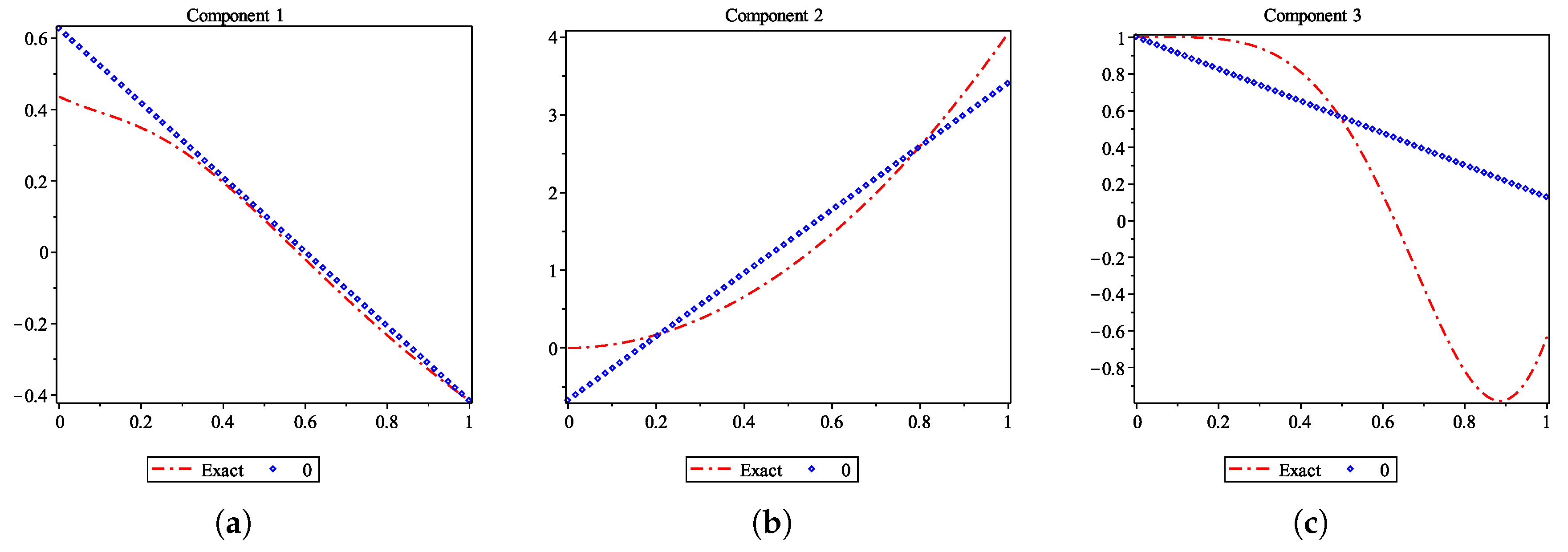
Substituting values (72) into formula (13) according to (61), we obtain the zeroth approximation $U_0=\mathrm{col}(U_{0,1},U_{0,2},U_{0,3})$, whose components $U_{0,i}$ represent the straight line segments joining the points $(0,{\xi }_i^{(0)})$ and $(1,{\eta }_i^{(0)})$, $i=1,2,3$. Although this linear approximation is very rough, it still provides some useful information on the localisation of the solution. On Figure 1, its graph is drawn together with that of the known exact solution (70). In particular, we have (see also Table 1) that

$$\begin{array}{cccccc}\hfill {\xi }_1^{(0)}-u_1^{*}(0)& \approx 0.194,\hfill & \hfill {\xi }_2^{(0)}-u_2^{*}(0)& \approx -0.681,\hfill & \hfill {\xi }_3^{(0)}-u_3^{*}(0)& =0,\hfill \\ \hfill {\eta }_1^{(0)}-u_1^{*}(1)& =0,\hfill & \hfill {\eta }_2^{(0)}-u_2^{*}(1)& \approx -0.652,\hfill & \hfill {\eta }_2^{(0)}-u_3^{*}(1)& \approx 0.777.\hfill \end{array}$$

The values of ${\xi }_3$ and ${\eta }_1$ in (71) are determined directly due to the form of the boundary conditions (69).

Figure 1. The zeroth approximation for problems (68) and (69).

Table 1. Values of the parameters computed from the approximate determining equations with $0\le m\le 10$ (11 nodes)

m	${\mathit{\xi }}_1$	${\mathit{\xi }}_2$	${\mathit{\xi }}_3$	${\mathit{\eta }}_1$	${\mathit{\eta }}_2$	${\mathit{\eta }}_3$
0	0.630827	−0.682613	1	−0.416667	3.40206	0.143882
1	0.516729	−0.0189486	1	−0.416667	4.08704	−0.412343
2	0.486264	0.00196245	1	−0.416667	4.04751	−0.675279
3	0.425443	−0.0020287	1	−0.416667	4.05544	−0.624705
4	0.439424	−0.00126683	1	−0.416667	4.05392	−0.634359
5	0.43643	−0.00141226	1	−0.416667	4.05421	−0.632516
6	0.437032	−0.0013845	1	−0.416667	4.05416	−0.632868
7	0.436914	−0.0013898	1	−0.416667	4.05417	−0.632801
8	0.436937	−0.00138879	1	−0.416667	4.05417	−0.632813
9	0.436932	−0.00138898	1	−0.416667	4.05417	−0.632811
10	0.436933	−0.00138895	1	−0.416667	4.05417	−0.632811
⋮	⋮	⋮	⋮	⋮	⋮	⋮
∞	0.436933	−0.00138889	1	−0.416667	4.05417	−0.63281

Furthermore, better approximations are obtained when we proceed to higher order iterations according to formula (14). For problem (68), (69), by virtue of (11), this formula means that the functions $u_m=\mathrm{col}(u_{m,1},u_{m,2},u_{m,3})$, $m\ge 1$, are constructed according to the recurrence relations

$$\begin{array}{cc}\hfill u_{m,1}(t,\xi ,\eta )& =u_{0,1}(t,\xi ,\eta )+{\tilde{q}}_1(t)+\frac{1}{6}{\int }_0^t{u}_{m-1,1}(1-s,\xi ,\eta )ds+\frac{2}{3}{\int }_0^t(s-1)u_{m-1,3}(1-s,\xi ,\eta )ds\hfill \\ \hfill & -\frac{t}{6}{\int }_0^1{u}_{m-1,1}(1-s,\xi ,\eta )ds-\frac{2t}{3}{\int }_0^1(s-1)u_{m-1,3}(1-s,\xi ,\eta )ds,\hfill \\ \hfill u_{m,2}(t,\xi ,\eta )& =u_{0,2}(t,\xi ,\eta )+{\tilde{q}}_2(t)-\beta {\int }_0^t{u}_{m-1,3}\left(\frac{s}{3},\xi ,\eta \right)ds-\beta t{\int }_0^1{u}_{m-1,3}\left(\frac{s}{3},\xi ,\eta \right)ds,\hfill \\ \hfill u_{m,3}(t,\xi ,\eta )& =u_{0,3}(t,\xi ,\eta )+{\tilde{q}}_3(t)+{\int }_0^t{u}_{m-1,2}(s,\xi ,\eta )ds-16{\int }_0^t{u}_{m-1,2}(\tau (s),\xi ,\eta )ds\hfill \\ \hfill & -t{\int }_0^1{u}_{m-1,2}(s,\xi ,\eta )ds+16t{\int }_0^1{u}_{m-1,2}(\tau (s),\xi ,\eta )ds\hfill \end{array}$$

for $t\in [0,1]$, $m=1,2,\cdots$, where $u_0=\mathrm{col}(u_{0,1},u_{0,2},u_{0,3})$ is the starting approximation (13) and the functions ${\tilde{q}}_i$, $i=1,2,3$, are computed by formula (12). A direct computation shows that, in this case, ${\tilde{q}}_i$, $i=1,2,3$, have the form

$$\begin{array}{cc}\hfill {\tilde{q}}_1(t)& =\frac{S(2t)-tS(2)}{144},\hfill \\ \hfill {\tilde{q}}_2(t)& =\frac{115223}{28800}{t}^2-\frac{115223}{28800}t+\frac{69}{200}\left(C\left(\frac{2}{3}t\right)-tC\left(\frac{2}{3}\right)\right),\hfill \\ \hfill {\tilde{q}}_3(t)& =\frac{S(2t)-tS(2)}{9}+\frac{tC(2\sqrt{2})-C(2\sqrt{2}t)}{\sqrt{2}}+\frac{t(t-1)}{12},t\in [0,1].\hfill \end{array}$$

The values ${\xi }_i$ and ${\eta }_i$, $i=1,2,3$, are kept as parameters when passing to the next iteration. The main computational work is to construct the functions $u_{m,i}(·,\xi ,\eta )$, $i=1,2,3$, analytically, for which purpose computer algebra systems are natural to be used.

Here, when carrying out computations according to the above recurrence relations, we use MAPLE and additionally simplify the task by using polynomial approximations in the spirit of [19] (more precisely, 9th order polynomials over the Chebyshev nodes; the interpolation nodes used in the course of computation are marked on the graphs). Carried out without interpolation (i.e., literally according to Section 7), the procedure allows achieving the required accuracy in a fewer number of steps but is more computationally expensive.

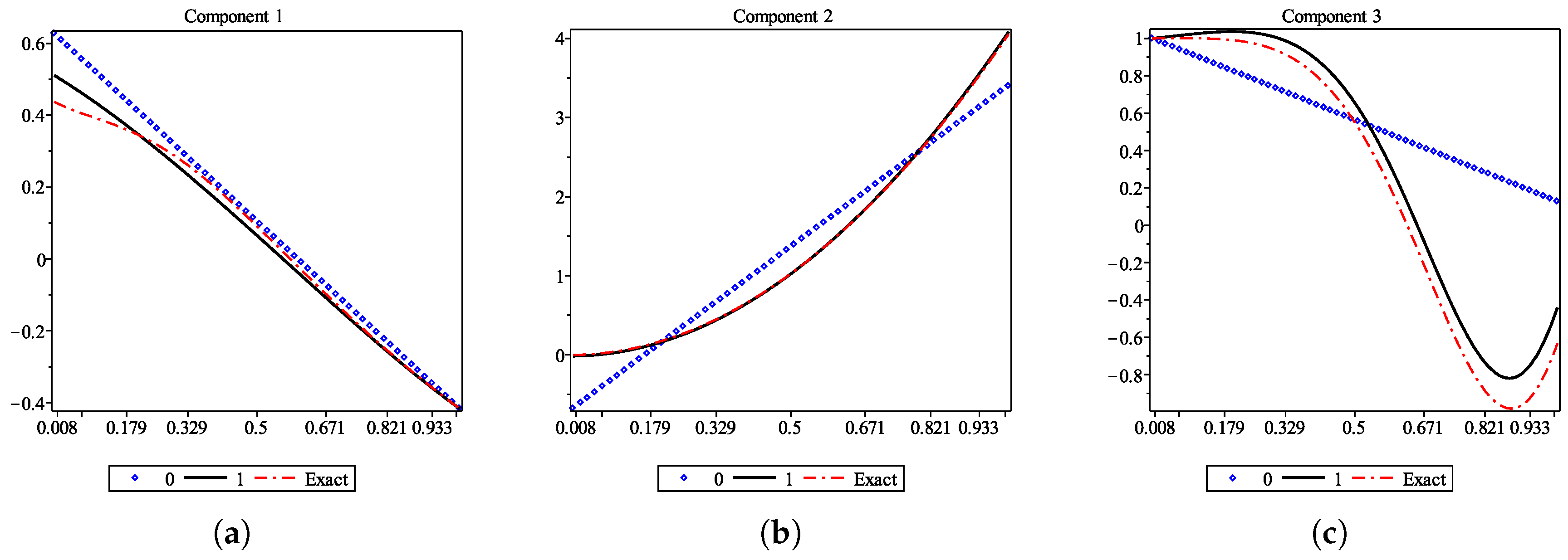
The rough zeroth approximation is improved when we start the iteration. To obtain the first approximation (63), we need to construct the functions $u_{1,i}(·,\xi ,\eta )$, $i=1,2,3$, and the corresponding first approximate determining system (62). Constructing system (62) and solving it numerically, we get the values

$$\begin{array}{cccccc}\hfill {\xi }_1^{(1)}& \approx 0.51673,\hfill & \hfill {\xi }_2^{(1)}& \approx -0.01895,\hfill & \hfill {\xi }_3^{(1)}& =1,\hfill \\ \hfill {\eta }_1^{(1)}& =-\frac{5}{12},\hfill & \hfill {\eta }_2^{(1)}& \approx 4.08704,\hfill & \hfill {\eta }_3^{(1)}& \approx -0.41232\hfill \end{array}$$

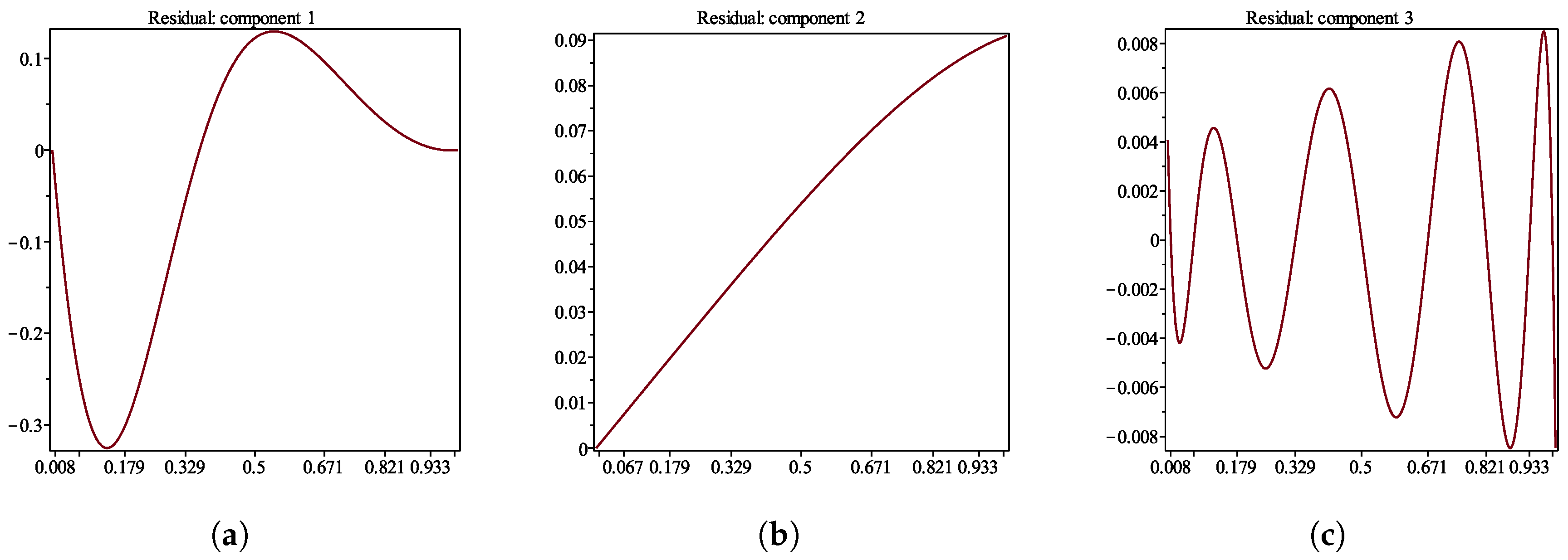
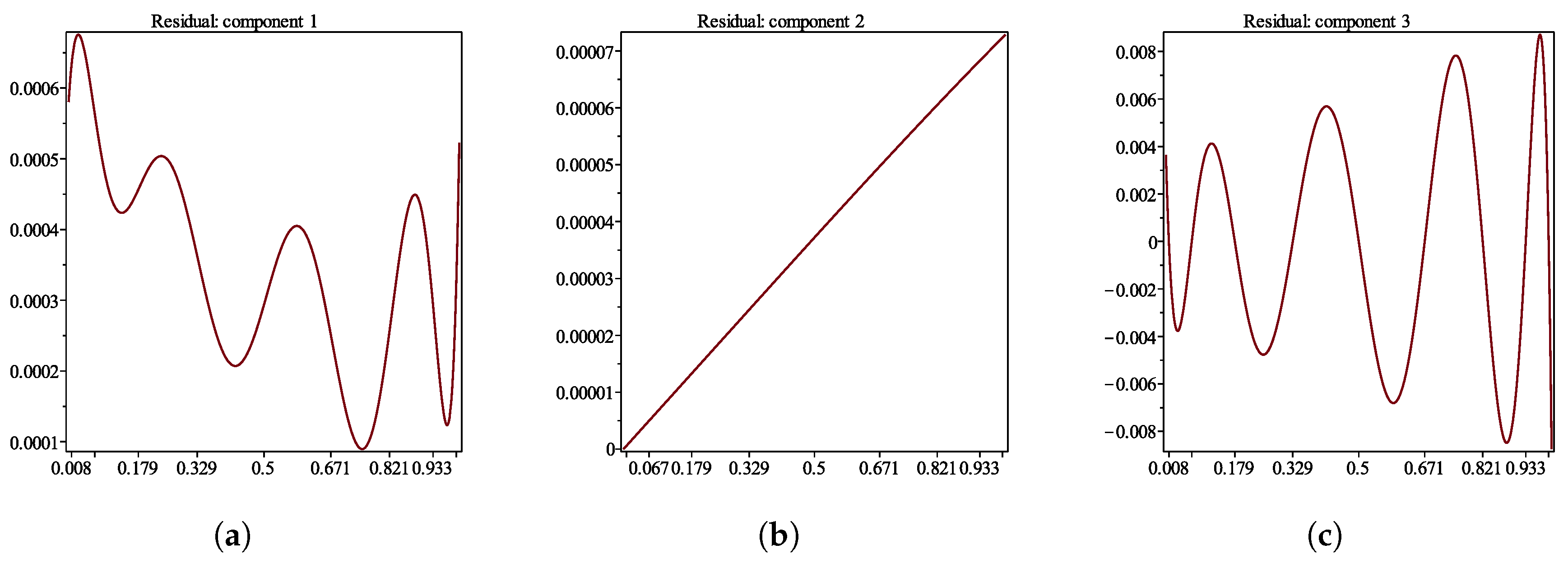
and, by (63), obtain the first approximation $U_1=\mathrm{col}(U_{1,1},U_{1,2},U_{1,3})$ the graph of which is shown on Figure 2. Checking the residual function $R_1$ corresponding to $U_1$ (Formula (66)) in Figure 3, we see that already the first approximation provides a reasonable degree of accuracy. Higher order approximations are obtained by repeating these steps for more iterations.

Figure 2. The first approximation for problems (68) and (69).

Figure 3. Residual of the first approximation.

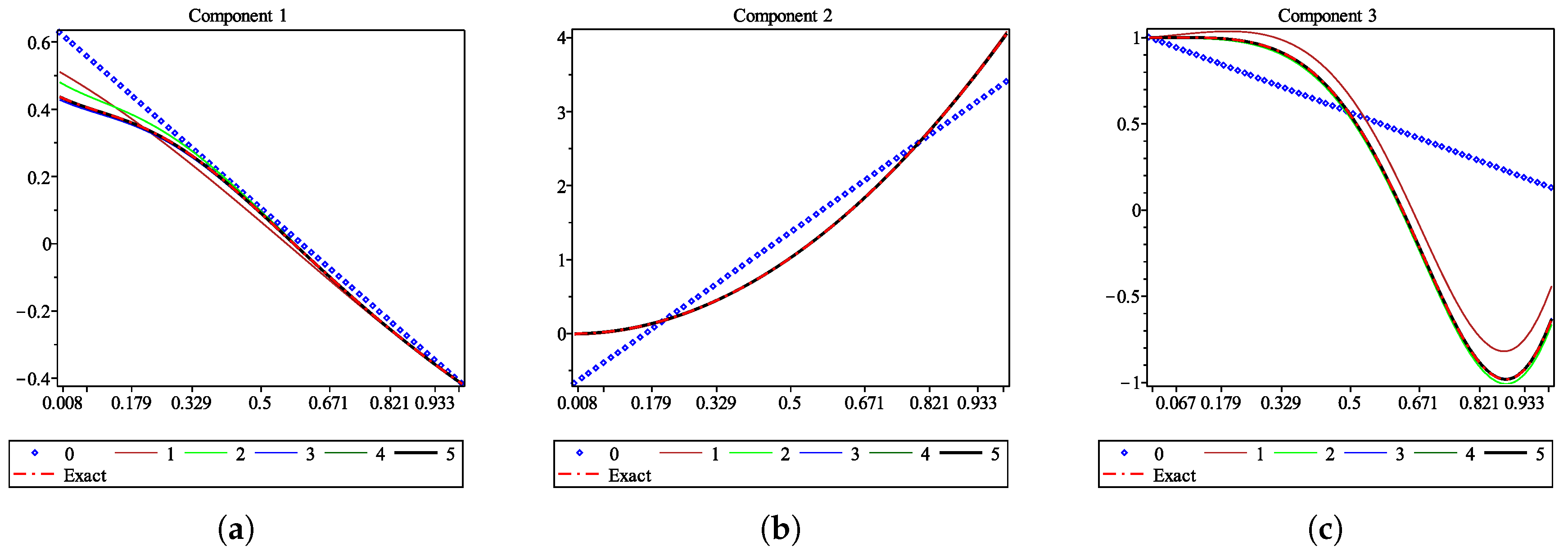
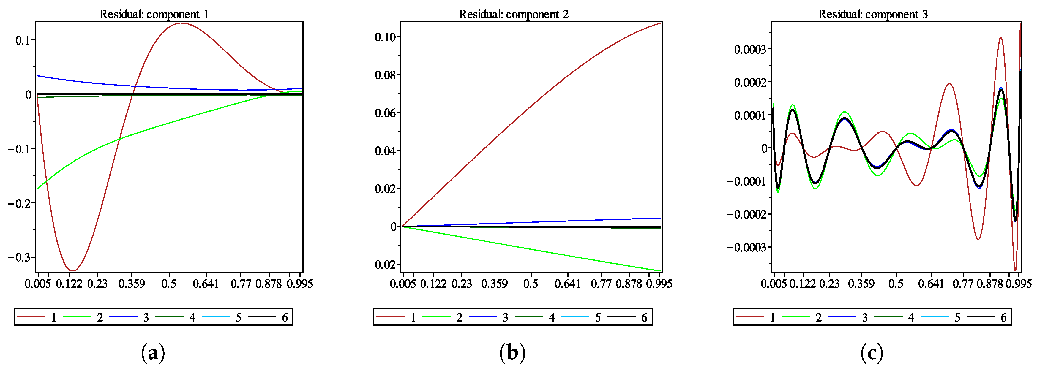
Figure 4 shows the graphs of several further approximations. We can observe that, starting from the third one, the graphs in fact coincide with one another. The maximal value of the residual $t\mapsto U_5^{\prime }(t)-(l{U}_5)(t)-q(t)$ of the fifth approximation $U_5$ is about $0.008$ (see Figure 5). The result is refined further when we continue the computation with more iterations. In this particular case, when interpolation is additionally used, this depends also on the number of nodes; increasing it from 9, e.g., to 11, we get the sixth approximation $U_6$ with the residual not exceeding $0.00025$ in every component. This is seen in Figure 6 (especially Figure 6c), where the graphs of the components of $R_m$, $1\le m\le 6$, are shown. The graph of $U_6$ does not optically differ from that of $U_5$ presented in Figure 4.

Figure 4. Several further approximations for problems (68) and (69).

Figure 5. Residual of the fifth approximation.

Figure 6. Residuals of the first six approximations (11 nodes).

The values ${\xi }^{(m)}$, ${\eta }^{(m)}$ obtained by numerically solving the approximate determining Equation (58) for $0\le m\le 10$ (with interpolation on 11 nodes) are collected in Table 1. In the last row of the table, for the sake of comparison, we give the values $u_i^{*}(0)$, $u_i^{*}(1)$, $i=1,2,3$, of the exact solution (70).

The approximations (64) are constructed in an analytic form; e.g., for the above-mentioned $U_6$, using Maple we obtain the explicit formulae

$$\begin{array}{cc}\hfill U_{6,1}(t)& \approx -4.042408471t^{11}+20.46952618t^{10}-37.43787653t^9+17.54308868t^8+38.65671249t^7\hfill \\ & -69.52449717t^6+43.70459764t^5-5.021255652t^4-6.515215520t^3+1.878014779t^2\hfill \\ & -0.5643854438t+0.4370323501,\hfill \\ \hfill U_{6,2}(t)& \approx 0.00004217847108t^{11}-0.0003918694568t^{10}+0.001582265878t^9-0.003636034946t^8\hfill \\ & +0.005193027536t^7-0.004701252907t^6+0.002625994458t^5-0.0008335495560t^4\hfill \\ & +0.0001241374492t^3+3.999981974t^2+0.055555553t-0.001384503,\hfill \\ \hfill U_{6,3}(t)& \approx 69.00767411t^{11}-297.1865115t^{10}+515.3651026t^9-495.0362578t^8+310.1738752t^7\hfill \\ & -122.453762t^6+30.80698530t^5-12.71224445t^4+0.3960898466t^3\hfill \\ & -0.01470825t^2+0.02088904869t+1\hfill \end{array}$$

for all $t\in [0,1]$.

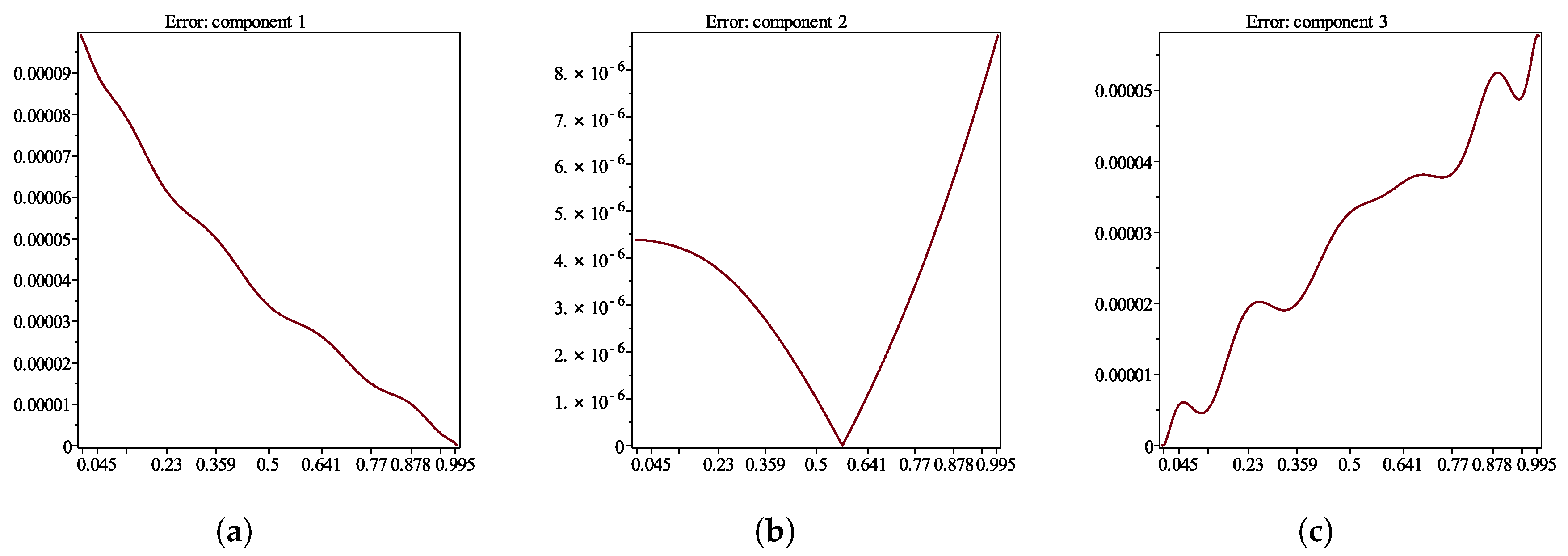
The accuracy of approximation of $u^{*}$ by $U_6$ can be verified in Figure 7, where the graphs of the corresponding error functions $t\mapsto |U_{6,i}(t)-u_i^{*}(t)|$, $i=1,2,3$, are shown. We can see that the maximal value of the absolute error does not exceed ${10}^{-4}$.

Figure 7. Error of the sixth approximation (11 nodes).