Article

An Improved Local Search Genetic Algorithm with a New Mapped Adaptive Operator Applied to Pseudo-Coloring Problem †

by
Monique Simplicio Viana
1,*,
Orides Morandin Junior
1 and
Rodrigo Colnago Contreras
2
1
Department of Computing, Federal University of São Carlos, São Carlos SP 13565-905, Brazil
2
Department of Applied Mathematics and Statistics, University of São Paulo, São Carlos SP 13566-590, Brazil
*
Author to whom correspondence should be addressed.
This paper is an extended version of our preliminary work “Contreras, et al. 2020”.
Symmetry 2020, 12(10), 1684; https://doi.org/10.3390/sym12101684
Submission received: 29 August 2020 / Revised: 22 September 2020 / Accepted: 30 September 2020 / Published: 14 October 2020
(This article belongs to the Special Issue Symmetry in Vision II)

Abstract

:
In many situations, an expert must visually analyze an image arranged in grey levels. However, the human eye has strong difficulty in detecting details in this type of image, making it necessary to use artificial coloring techniques. The pseudo-coloring problem (PsCP) consists of assigning to a grey-level image, pre-segmented in K sub-regions, a set of K colors that are as dissimilar as possible. This problem is part of the well-known class of NP-Hard problems and, therefore, does not present an exact solution for all instances. Thus, meta-heuristics has been widely used to overcome this problem. In particular, genetic algorithm (GA) is one of those techniques that stands out in the literature and has already been used in PsCP. In this work, we present a new method that consists of an improvement of the GA specialized in solving the PsCP. In addition, we propose the addition of local search operators and rules for adapting parameters based on symmetric mapping functions to avoid common problems in this type of technique such as premature convergence and inadequate exploration in the search space. Our method is evaluated in three different case studies: the first consisting of the pseudo-colorization of real-world images on the RGB color space; the second consisting of the pseudo-colorization in RGB color space considering synthetic and abstract images in which its sub-regions are fully-connected; and the third consisting of the pseudo-colorization in the Munsell atlas color set. In all scenarios, our method is compared with other state-of-the-art techniques and presents superior results. Specifically, the use of mapped automatic adjustment operators proved to be powerful in boosting the proposed meta-heuristic to obtain more robust results in all evaluated instances of PsCP in all the considered case studies.

1. Introduction

There are situations of visual data analysis in which an expert must extract complex considerations from images originally arranged in gray levels. In these situations, it is common to use the most diverse tools, but the visual analysis is almost always present. For example, we can highlight some recent challenges to detecting edges in sonar images [1], to detecting weapons in baggage [2], to visually analyze medical images [3,4,5,6,7], to conduct visual routines in remote sensing [8,9], to detect crashes in wire ropes [10], among other situations. Still, the human eye is not able to detect many details in an image colored with different shades of the same color [11,12] because the human brain has difficulty in the task of recognizing signals defined by similar frequencies. To solve this issue, one of the techniques most commonly used in specialized literature is the artificial attribution of colors in order to obtain a visual enhancement in certain regions of the image.
In this case, it is necessary to define a set of colors for different regions of the original grey-level image, so that these colors are as visually dissimilar as possible and make the task of visually differentiating neighboring regions in an image easier. This problem is known in the specialized literature as pseudo-coloring problem (PsCP), or as the definition of color sets of high visual contrast [13]. This is a problem in which it is necessary to establish a finite set of elements belonging to a given color space, such that these elements are as far distant as possible according to some measure of distance. In this way, we can see that PsCP is an optimization problem. In addition, if the set of colors to be calculated is defined by a few elements, then PsCP can be solved exactly by greedy algorithms; however, if it is necessary to define a reasonably large amount of colors, the problem may not be solved. This is because PsCP is a combinatorial problem of the well-known class of NP-Hard problems. For this reason, many authors have proposed to solve it with the use of inexact methodologies; that is, with the use of meta-heuristics. As an example, we can highlight the work of Radlak and Smolka [14], who solve PsCP with the use of a GA. However, it is known that this meta-heuristic can have difficulty in solving complex combinatorial problems since it is common to be stuck in local optima and present premature convergence [15].
In the literature, we find strategies that can be used in GA to make it more efficient and less susceptible to the difficulties mentioned. For example, Asadzadeh [16] proposed the use of local search strategies across all standard GA operators. In addition, the author also defined an operator specialized in massive local search, the “elite local search procedure”. The methodology is used in the job shop scheduling problem, which is also an NP-Hard combinatorial problem. These strategies proved to be effective and surpassed the other evolutionary techniques considered. Therefore, one of the proposals of our work is to use these strategies in GA and adapt them to be able to solve PsCP. In addition, we also propose to add in GA a step of auto adjustment of parameters [17,18], since the use of this type of technique in the meta-heuristic in question proved to be useful when used to solve other NP-Hard problems [19,20].
This paper is an extended version of our preliminary work [21]. In this text, we generalize the adaptive rules of our technique using mapping functions that automatically update the parameterization of the meta-heuristic. We also added a section of related works that address the different types of pseudo-colorization in the specialized literature and a section that details the methodology followed for the resolution of PsCP by the proposed method. This text is richer in detail since we add descriptions of all the routines of operators of the method through flowcharts and algorithms with comments. The computational experiments were also updated with more comparisons taking into account more recent works.
The paper is organized into 7 sections. Specifically, in Section 2, we discuss the different types of approaches that involve pseudo-colorization methods available in the current literature. In Section 3, we describe the mathematical formulation of PsCP. In Section 4, we present the methodology used in this work to solve the PsCP. The formulation of the proposed algorithm and the details of all its operators are presented in Section 5. The proposed method is evaluated in three test scenarios and the experimental results obtained are presented in Section 6. The manuscript ends with conclusions and proposals for future work in Section 7.

2. Related Works

Associating different colors for partitions of an image is a problem from the well-known four-color theorem [22], which establishes that, using four distinct colors, there is at least one possible color configuration in which the vertices of any planar graph can be colored so that no pair of neighboring vertices are colored with the same color. From this result, the graph coloring theory was created, which concentrates around 200 problems still unsolved [23]. One of these problems is the pseudo-coloring problem (PsCP), which belongs to the class of NP-Hard problems [24] and that we focus on this work.
PsCP can also be interpreted to keep semantic information during the association of colors in regions of images. In this case, it is considered that the objective of the problem is to convert an image available only in grey-level to a color version so that the color associations make sense and preserve the original meaning of the represented components in the image [25]. One example in this research field is [26], where the PsCP was addressed with the use of an architecture of multiple Generative Adversarial Networks (GANs). The method, called Multi-GANs, has obtained results with acceptable colors, presenting more realistic characteristics and meaning for the images generated. On the other hand, Fang, et al. [27] addresses the problem of image colorization by exploring measures of self-similarity and consistency constraints in the resolution of superpixels. More recently, Wan, et al. [28] proposed a fully automatic method using neural networks and optimization to treat image colorization. For a more comprehensive overview, we recommend the work of Li, et al. [29], who present the most updated and deep review in this specific field.
In this work, our advances are contained in a sub-area of PsCP known as color coding [30]. In this type of research, the problem of associating artificial colors to sub-regions of a grey-level image is a problem of combinatorial optimization defined in a graph [31], in which it is necessary to establish a color for each sub-region considering a fixed set of colors and in such a way that the colors chosen are as visually dissimilar as possible [32]. In other words, the objective of these problems is to determine a high contrast set of colors [33]. In this field, one of the most recognized works is the paper by Carter and Carter [13], which was the first work to propose a heuristic search that aimed to explore the RGB color space for a set of colors that was as dissimilar as possible taking into account distances in CIELUV space. In this case, the algorithm starts with several points in RGB, defined through the Grassman’s laws [34], and in each iteration, one of these points was moved away from the others as much as possible, so that, at the end of the method, all points were spread out in space quasi-optimally. Glasbey, et al. [35] show an extension to this heuristic formulated by sequential sets. In detail, the authors present a method of greedy behavior that begins with a set formed only by the white color and to this set is added the most dissimilar color available in the entire color space, giving rise to another set of two colors and so on until the set has a color for each sub-region to be colored. In addition, to determine high contrast sets and taking into account multiple illuminant configurations, Bianco and Citrolo [36] proposed a heuristic that performs local searches in the neighborhood of possible PsCP solutions until no configuration that is better than the previous configuration is found. The authors compare the performance of their technique with two basic meta-heuristics also proposed in their work: simulated annealing (SA) [37] and genetic algorithm (GA) [38]. A generalization of this local search heuristic is proposed in the form of an unsupervised high-contrast coloring (HCC) algorithm [39].
Bioinspired meta-heuristics have also achieved advances in PsCP by determining high contrast sets of colors. For example, Radlak and Smolka [14] proposes a GA that performs searches in the RGB space in order to artificially color a pre-segmented grey-level image. In detail, the authors divide the population of the algorithm into three sub-populations: one specific for the component R; another for component G; and another for component B. In the same work, a new quantitative measure of performance comparison is also proposed, which is described in details in the next sections of our work. More recently, we proposed in our preliminary work [21] a new GA with local search and adaptive operators specialized in solving the PsCP. In this text, we present the expansion of this technique, in which the adaptive operator makes use of mapping functions to update the mutation and crossover rates during the method iterations.
In the next section, we present in detail the mathematical formulation of PsCP treated in this work.

3. Mathematical Formulation of Pseudo-Coloring Problem

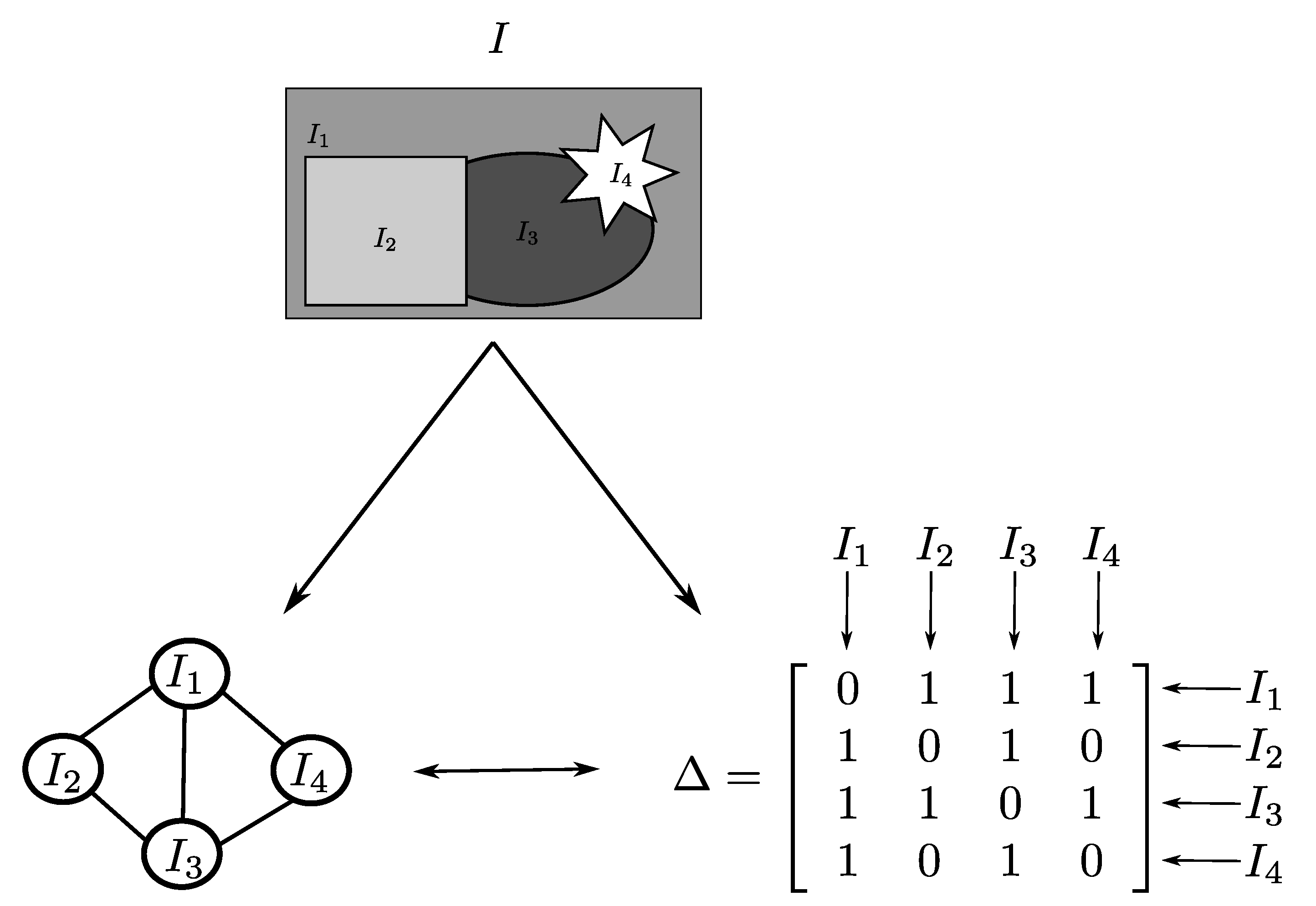
To define PsCP, we will use in this work a model similar to that used by Radlak and Smolka [14]. For this, we will consider that we have as input a grey-level image I, pre-segmented in K disjunct sub-regions, and we will obtain as output a set of K colors that are as visually dissimilar as possible in neighboring regions. Mathematically, let I 1 , I 2 , …, I K be the pre-segmented sub-regions of I, and let Δ = ( δ i , j ) i , j = 1 K be the neighborhood matrix representing the connections between those sub-regions whose coordinates δ i , j are defined as follows in the Equation (1):
δ i , j = 1 , if   I i is   neighbor   of   I j in   I , 0 , if   I i is   not   neighbor   of   I j   in   I   or   if i = j .
In other words, the neighborhood matrix Δ describes the arrangement of all sub-regions in I and can be interpreted as the adjacency matrix of a graph that represents the connections between the sub-regions. This information is very important to solve the PsCP, since sub-regions that are neighbors must be colored with the most different colors possible, while sub-regions that are not connected can be colored with similar colors without much loss to the visualization. In Figure 1, we present a schematic with a grey-level image I pre-segmented in K = 4 sub-regions, the neighborhood matrix Δ defined by the positioning of these sub-regions and the graph that this matrix defines.
Thus, to solve the PsCP, we have to determine a set of K colors C = { c 1 , c 2 , , c K } to pseudo-coloring all the sub-regions of I, with neighborhood matrix Δ = ( δ i , j ) i , j = 1 K , such that the value of the function F Δ of Equation (2), which can be interpreted as the lowest distance between the colors of all neighbor sub-regions of I, is the greatest possible value, configuring this version of the PsCP in a max–min optimization problem.
F Δ ( C ) : = min d ( c i , c j ) | δ i , j 0 , c i , c j C ,
in which d ( · , · ) is a distance function in some color space. Even though d ( · , · ) can be defined as any distance between two given colors, it is common to define the distance function d ( · , · ) to be the Euclidean distance between colors in the perceptually uniform color space CIELab (Commission Internationale de l’Eclairage) [40] with illuminant D50, since this space is favorable for performing tasks of visual distinction of colors [41]. In this case, mathematically, the distance measurement between two colors c i and c j is defined in Equation (3).
d : Y × Y R + ( c i , c j ) L i L j 2 + a i a j 2 + b i b j 2 ,
in which Y is some color space, and ( L i , a i , b i ) and ( L j , a j , b j ) are the CIELab components of the colors c i and c j , respectively.
We are defining the PsCP without any specification regarding the color space since our methodology does not restrict the F Δ domain. In this way, each color c i of the problem can be interpreted as belonging to any color space. For example, if the color space considered is the Y = sRGB space, then each color c i must be represented by the three components R i , G i and B i belonging to the set { 0 , 1 , 2 , , 255 } , so whereas these three components represent, respectively, the intensity of red, the intensity of green and the intensity of blue of the color c i . Therefore, the sub-region I i must be colored with the color ( R i , G i , B i ) . As a consequence of this, the set of all K colors C would be a subset of { 0 , 1 , , 255 } 3 · K .
Finally, the PsCP approached in this work consists of finding the set of colors C * with the greatest possible dissimilarity between its elements c 1 , c 2 , , c K and that, therefore, is a solution to the optimization problem presented in Equation (4).
C * = argmax C F Δ ( C ) subject to C Y K .

4. Methodology

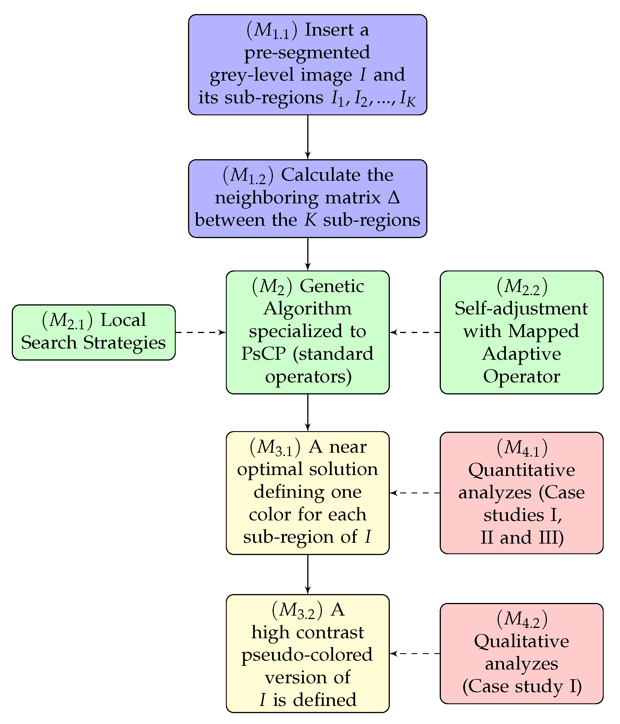
To solve PsCP, we propose an approach that is configured mainly by four steps:
M 1
Domain definition: This phase consists of defining the image in grey-levels that must be pseudo-colored by our technique.
M 1.1
However, all results can be easily extended to consider classes of images that have not passed any segmentation process, given the advances achieved in recent years in the area of image segmentation [42,43,44]. This type of consideration is outside the scope of the paper, so we will assume in this work that the method must work on an image in grey levels I pre-segmented into K sub-regions.
M 1.2
Once we have the pre-segmented image I, we need to define the neighborhood matrix Δ of this image so that the algorithm can perform the optimization having the information of which subregions of I are neighbors to each other and, consequently, they are assigned different colors.
M 2
Proposed optimization method: In this step of the methodology, we use the proposed meta-heuristic, which consists of a genetic algorithm that was specifically designed to search in a color space for an optimal solution for PsCP. Our main contributions to the method are given in the form of two operators:
M 2.1
Local search strategies: As in our preliminary work [21], we will also use local search strategies in our GA in two operators: the mutation operator and an exclusive operator dedicated to conducting a local search with massive behavior.
M 2.2
Adaptive rules: In this text, we generalize the use of the rules for self-adaptation of parameters proposed in our preliminary work [21] having as inspiration ideas that have been successfully used in other classes of combinatorial optimization problems [20]. In this case, we make use of mapping functions to automate the way that mutation and crossing rates are updated in the course of GA iterations.
M 3
Algorithm responses: After the optimization process carried out by our technique, we obtain two types of responses: a numerical and vector solution in the K-dimensional color space ( M 3.1 ) and the pseudo-colored image ( M 3.2 ). In the first case, we have numerical and quantitative information on how different are the colors attributed to I, calculated from the measures of Radlak and Smolka [14]. In the second case, the method must establish the pseudo-colored version of I from the obtained vector solution.
M 4
Validation scenarios: In our methodology, we will validate the solutions found by our meta-heuristics in a quantitative ( M 4.1 ) and in a qualitative ( M 4.2 ) ways through three different case studies (CS):
-
CS I: In the first CS, we will compare the quantitative and qualitative results obtained by our method that represent information on how distant the colors attributed to the I regions are in the CIELAB space and compare the results with the most recent color-coding techniques available in the specialized literature.
-
CS II: In the second CS, we will compare the quantitative results obtained by our method in 24 synthetic and abstract unreal images in comparison to the other existing techniques in this field of study.
-
CS III: In the third CS, we we will compare the quantitative results obtained by our method considering the Munsell atlas color space in comparison to the other existing techniques in the specialized literature.
In Figure 2, we present a pipeline of the proposed methodology to solve PsCP. So that the steps of domain definition are colored blue, the steps of the proposed optimization method are colored green, the steps of algorithm response are colored yellow and the steps of validation scenarios are colored red.

5. Mapped Local Search Adaptive Genetic Algorithm for PsCP

In this section, we present the explanation of our method, which was developed specifically to solve PsCP. All operators that make up the proposed meta-heuristic are discussed in detail. In addition, to facilitate the reproduction of the technique, pseudo-codes and operating schemes of all operators are presented throughout the manuscript. We highlight as the main innovations of our approach the use of local search strategies in GA; in particular, the definition of a massive local search operator, and the use of adaptive rules in order to perform parameter tuning. To the best of our knowledge, this type of strategy, although widely used in other combinatorial optimization problems, has not yet been employed in the PsCP solution. In addition, in this extended version of our work, we generalize the adaptive operator through antisymmetric mapping functions. Thus, the main contributions of our work are contained in the following topics:
  • A new meta-heuristic specialized in solving the PsCP with local search strategies in all operators. Inspired by the works of Asadzadeh [16] and Viana, et al. [45], we developed a massive local search operator that explores the best individual neighborhood.
  • A new self-parameter adjustment operator [17] to avoid well-known problems in GA such as premature convergence and getting stuck in local optima. In addition, we present the generalization of our preliminary adaptive strategy from [21] using mapping functions, which proved to be favorable in studies related to other types of combinatorial optimization [19,20].
  • The advancement of experimental results in benchmarks that define the state-of-the-art.

5.1. Chromosome Decoding

A possible solution for the PsCP is defined by a set of K colors to be associated with the regions of a pre-segmented gray-level image I. To make this computationally efficient, the chromosome must be the vectorized version of the color set C = c 1 , c 2 , , c K Y K . In this way, each gene on this chromosome is formed by a color c i that must be used to coloring the sub-region I i . Mathematically, the chromosome decoding adopted in this work that should represent the set C is the vector C defined in Equation (5).
C = c 1 , c 2 , , c K ,
in which c i Y is the color to be associated with the region I i .
As an example, if the considered color space is the sRGB, then the chromosome will be in the form: C = R 1 , G 1 , B 1 , R 2 , G 2 , B 2 , , R K , G K , B K , with R i , G i , B i 0 , 1 , 2 , 3 , , 255 for all i.
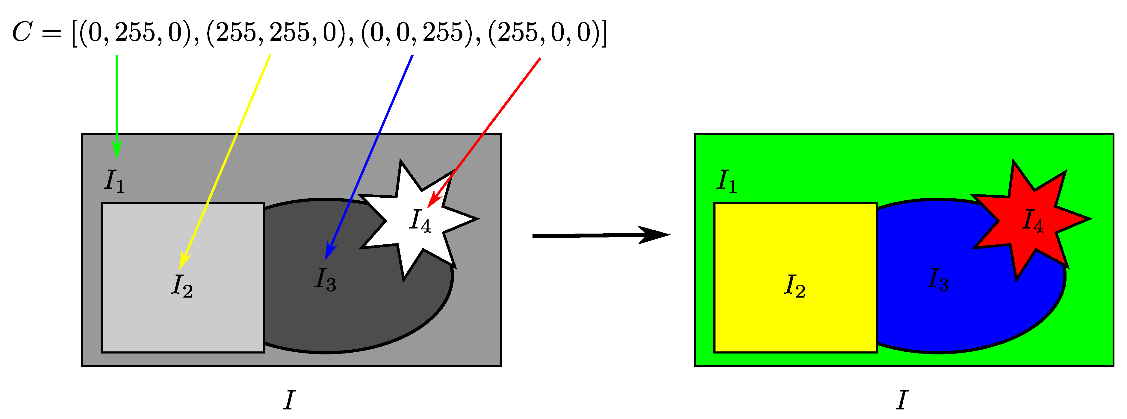
In general, the chromosome used in this work is a vector in the space R n · K , with n being the dimension of the space Y . Therefore, there is an ordering between the C coordinates that must be taken into account to coloring the I sub-regions, since the first n coordinates of the chromosome C (first gene) represent the components of the color c 1 that should be used to coloring the I 1 subregion, the following n coordinates of C (second gene) represent the components of the color c 2 that should be used to coloring the subregion I 2 , and so on. In Figure 3, we present an example that outlines, according to the proposed decoding, the relationship between the genes of a chromosome C, with Y = sRGB, and the pseudo-coloring process in a pre-segmented grey-level image I in K = 4 sub-regions.

5.2. Fitness Function

According to the decoding proposed in Section 5.1, we can naturally define the fitness value associated with a C chromosome as an isomorphism of the function F (Equation (2)), computationally efficient, of its representation as a set of colors C . Mathematically, given a grey-level image I with neighborhood matrix Δ , we define the fitness value of a chromosome C = [ c 1 , c 2 , , c K ] Y K the function F ¯ Δ , presented in Equation (6).
F ¯ Δ : Y K R + ( c 1 , c 2 , , c K ) F ¯ Δ c 1 , c 2 , , c K : = F Δ c 1 , c 2 , , c K .
It is worth highlighting some considerations regarding the function F ¯ Δ :
  • Both F ¯ Δ and F Δ are defined taking into account the neighborhood matrix Δ . That is, both functions are defined from the image structure that we intend to color.
  • The main difference between F ¯ Δ and F Δ is that the first one takes into account the order of the coordinates in the chromosome C, while the second one acts on a set C . Didactically, it is simpler to reproduce F ¯ Δ and, therefore, we define the fitness function in this way.
  • The meta-heuristic that finds the greatest values assumed by F ¯ Δ will find possible solutions to the problem presented in Equation (4), since these two situations consist of determining K colors with the greatest possible visual dissimilarity. In this way, the feasibility and the equivalence of the problem are maintained.

5.3. Selection Process

The selection step in an evolutionary algorithm like GA is very important since it is from this routine that we simulate the Darwinian phenomenon of “natural selection” [38], making good solutions more likely to perpetuate their genes. In the case of GA, selection strategies are used to define which chromosomes will pass through the crossover operator and which chromosomes will survive in the stage of creating a new population. This step of the method takes into account the numerical fitness value of each chromosome, and since the PsCP is a maximization problem, the higher the fitness value of a chromosome, the greater the chance of being selected. In detail, we will use in this work the strategy known as roulette wheel selection [46] in the case of the choice of individuals for the crossover operator, and the roulette wheel selection retaining the best individual of the population [47] in the case of the generation of new population.

5.4. Crossover Operator

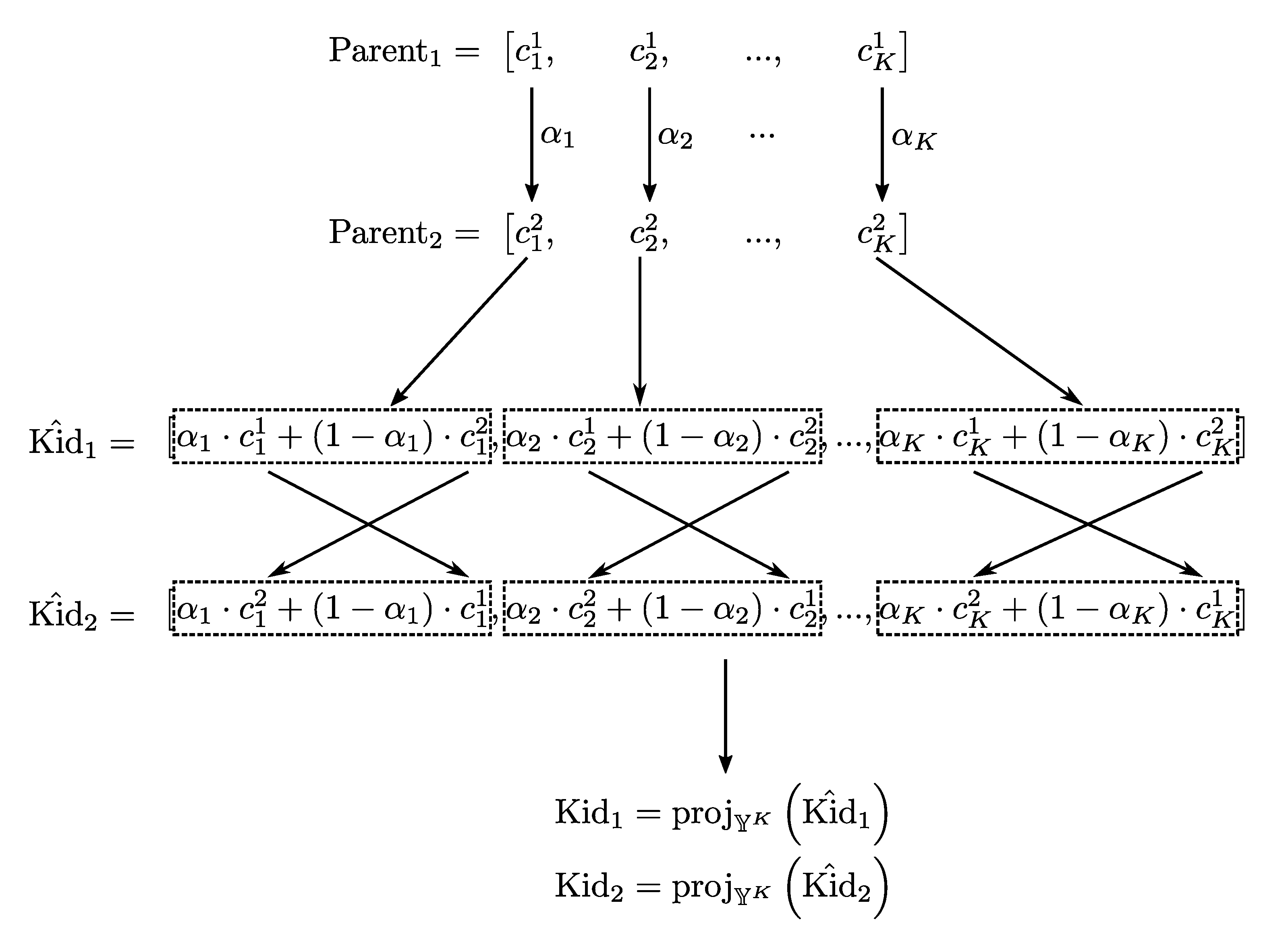
It is at this stage of the method that we will carry out the genetic combination method between the chromosomes selected in the previous section. In this case, the parent chromosomes must be combined two by two and this process should result in two child chromosomes. In order that no generated chromosome is outside the limits that define the Y color space, we propose to use an adaptation of the well-known convex crossover [48], in which the convex combination of two parent-chromosomes, Parent 1 and Parent 2 , is made, resulting in two offspring-chromosomes, Kid 1 and Kid 2 , according to Equation (7) given below.
Kid 1 = pro j Y K ( α T · Parent 1 + ( 1 α ) T · Parent 2 ) ,
Kid 2 = pro j Y K ( ( 1 α ) T · parent 1 + α T · parent 2 ) ,
where 1 is the R n · K × 1 vector whose coordinates are all equal to 1 and α is an R n · K × 1 vector whose coordinates are taken randomly between [ 0 , 1 ] .
It is worth mentioning that we are using a projection function to ensure that Kid 1 and Kid 2 are, in fact, feasible values of colors in the space Y . In general, this function projects the results obtained by the convex combination between parent 1 and parent 2 of the R n · K space for the respective closest vectors in the Y K space, with n being the dimension of Y . This projection, defined in Equation (8), determines the generated offsprings: Kid 1 and Kid 2 .
pro j Y K · : R n K Y K ( x 1 , x 2 , , x n K ) arg min c 1 , c 2 , , c K Y K ( x 1 , x 2 , , x n K ) c 1 , c 2 , , c K 2 .
Note that in most cases, the projection function pro j Y K ( · ) has an explicit and very simple form. For example, in the special case where Y = sRGB , then pro j Y K ( · ) = round   ( · ) , in which round   ( · ) is the well-known approximation function to the nearest integer.
A schematic of our crossover technique is presented in Figure 4.

5.5. Mutation Operator

The mutation operator proposed in this work uses inspiration from the local search strategies presented by Asadzadeh [16] and Ombuki and Ventresca [49]. In fact, we propose an improvement based on the union between the techniques of these two works. In this case, Asadzadeh [16] proposes that successive local searches be carried out on the individuals in the mutation operator, while Ombuki and Ventresca [49] suggests that, in some cases, successive local searches are carried out on the individual and in other cases, only a simple mutation is applied on the individual. In this way, our mutation operator is divided into two subroutines:
  • Mut 1 : In this routine, a mutation function is randomly taken into a set of mutation functions, and, using this function, N Mut 1 perturbations are performed on the chromosome, so that the good perturbations are maintained and the bad ones are ignored.
  • Mut 2 : In this routine, a simple Gaussian mutation is applied to the chromosome.
An individual who is generated on the crossover operator has a p mut chance of passing through the mutation operator. In addition, to control the use of the Mut 1 and Mut 2 subroutines, all individuals selected for the mutation will be perturbed according to only one of these subroutines. Thus, these individuals have a p LS chance of being perturbed according to the Mut 1 subroutine and, consequently, these individuals have a chance 1 p LS of being perturbed according to the Mut 2 subroutine.
To model this operation, a group of mutation functions given in the form of f mut ( · , · ) is used in Equation (9).
f mut : Y × { 1 , 2 , , n · K } 2 Y C , ( i , j ) f mut C , i , j ,
where n is the dimension of Y .
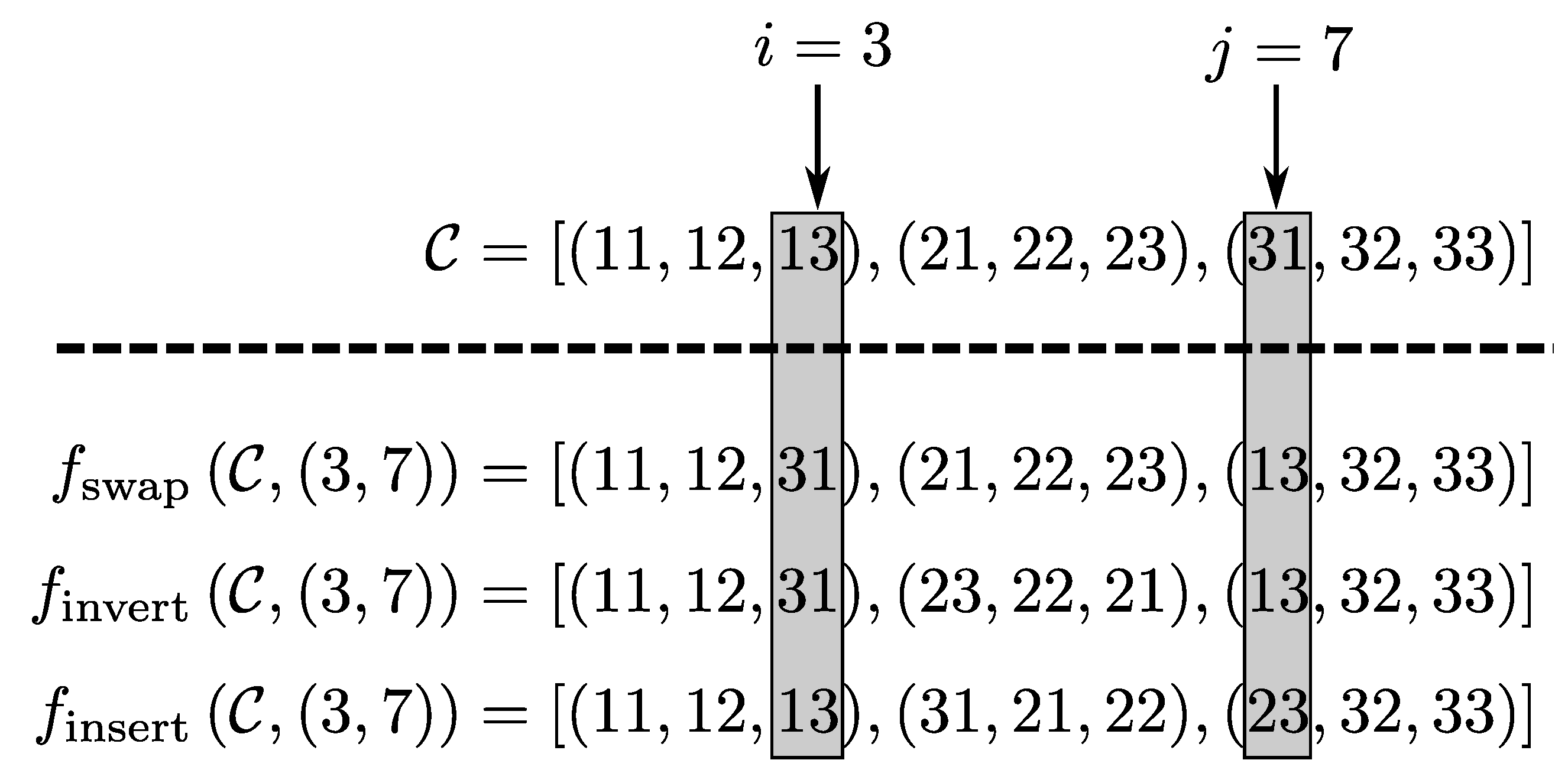
The definition of the Mut 1 subroutine establishes that it is necessary to randomly choose a mutation function from a group of mutation functions. Thus, it is necessary to define a set formed by possible mutation functions. In this work, as we are going to solve the NP-Hard combinatorial problem PsCP, we are going to use mutation functions widely used in solving problems of this type. In this case, we will use the functions [50]: f swap ( · , · ) , f invert ( · , · ) and f invert ( · , · ) . These functions affect perturbations on the chromosome in order to shift some of its coordinates. In Figure 5, we can see the result of the disturbance made by all these functions on the same individual considering the Y = sRGB color space and considering that the image to be pseudo-colored is pre-segmented in K = 3 sub-regions. Certainly, feasibility is maintained in cubic spaces defined by intervals of the same range, as is the case of sRGB space. However, if at the end of the entire mutation procedure, the generated individual is outside the color space, then it is necessary to make use of the projection function on the mutant individual.
In Mut 2 , we propose to use only one mutation function. In this case, we apply a simple Gaussian perturbation [51] on the color adding a Gaussian noise in each color component. In this way, all genes in the chromosome receives a slightly random increase or decrease.
Specifically, we will suppose that the Y can be represented or approximated to a cube in Y R n , such that Y : = [ l 1 , L 1 ] × [ l 2 , L 2 ] × × [ l n , L n ] . In this way, if one color c i is in Y , then c i = ( c i , 1 , c i , 2 , , c i , n ) and l j c i , j L j for all j { 1 , 2 , , n } . For example, if we choose Y as being the sRGB color space, then all the colors would have three components ( n = 3 ) and all ranges would be defined by the following lower and upper bounds: l 1 = l 2 = l 3 = 0 and L 1 = L 2 = L 3 = 255 .
Finally, we can define the mutation function used for this situation as the function f Gauss ( · ) : Y K Y K defined in Equation (10).
f Gauss c 1 c 2 c K T = f Gauss c 1 , 1 c 1 , 2 c 1 , n c 2 , 1 c 2 , 2 c 2 , n c K , 1 c K , 2 c K , n T : = Proj Y K c 1 , 1 + β 1 c 1 , 2 + β 2 c 1 , n + β n c 2 , 1 + β n + 1 c 2 , 2 + β n + 2 c 2 , n + β n + n c K , 1 + β ( K 1 ) · n + 1 c K , 2 + β ( K 1 ) · n + 2 c K , n + β ( K 1 ) · n + n T ,
in which β ( r 1 ) · n + j is a random number obtained from a normal distribution with mean 0 and standard deviation equals to L j l j 10 , for all r { 1 , 2 , , K } and j { 1 , 2 , , n } . We chose this configuration, as it is a simple and well-established strategy in the specialized literature on gaussian disturbances in GAs, as initially proposed by Hinterding [52]. Note that we are using the projection function in the final disturbance of the chromosome since the addition of gaussian noise can remove the chromosome from the feasible color space.
In the Algorithm 1, the proposed mutation procedure is summarized.
Algorithm 1 Proposed mutation operator.
Input: P kids Offsprings generated in crossover
F ¯ Δ Fitness function
p mut Probability of mutation
p LS Probability of Mut 1
N Mut 1 Number of mutation function applications for Mut 1
  1: f mut : = rand _ take   { f swap , f invert , f insert }            ▹ The function rand _ take · randomly returns an element from a set.
 2: P mut : = { }
 3:for C P kids do
 4:    if rand ( [ 0 , 1 ] ) p mut then             ▹ Apply mutation in p mut percent of kids.
 5:        break
 6:    else if rand ( [ 0 , 1 ] ) p LS then                ▹ Apply Mut 1 in p LS percent of cases.
 7:         F C : = F ¯ Δ ( C )
 8:        for k : = 1 to N Mut 1 do                         ▹ Apply f mut N Mut 1 times.
 9:            i : = rand _ take { 1 , 2 ,   , 3 K }
10:            j : = rand _ take { 1 , 2 ,   , i 1 , i + 1 ,   , 3 K }
11:            C ^ : = f mut C , ( i , j )
12:            F C ^ : = F ¯ Δ ( C ^ )
13:           if F C ^ F C then           ▹ If the perturbation is beneficial, then it must be maintained.
14:                C : = C ^
15:                F C : = F C ^
16:           end if
17:        end for
18:    else                            ▹ ( Mut 2 ) Apply f Gauss only once.
19:         C : = f Gauss C
20:    end if
21:     P mut : = P mut { C }
22:end for
Output: P mut Population of mutated individuals

5.6. Massive Local Search Operator

The main objective of a massive local search operator [45] is to perform a more elaborate and systematic search around good solutions. Already used to solve other combinatorial works, the idea behind this type of operator is that we are more inclined to find better solutions when examining the neighborhood of chromosomes with better fitness than when investigating randomly in space. For example, Asadzadeh [16] proposes to apply this strategy to the best individual in the population. Specifically, the author performs, in a controlled manner, successive disturbances with the function f swap ( · , · ) so that all the coordinates of the chromosome can be swapped if convenient. In this work, we propose a new massive local search operator that specializes in disturbing, one by one, the colors represented by the genes of the best individual in a population. In detail, we will consider that C Best = ( c 1 , c 2 , , c K ) is the best individual in a population and, in sequence, for each color c i represented by the genes of C Best we will perform the following four steps:
  • Step 1: The color c i receives a random increase, making it lighter.
  • Step 2: The perturbation is maintained only if it is beneficial, increasing the fitness value of C Best .
  • Step 3: If c i was not modified in the previous step, then a random decrease in c i is applied, making it darker.
  • Step 4: The perturbation should be maintained if it is beneficial.
Therefore, in the Algorithm 2, we can see details about our proposed massive local search operator to solve the PsCP.
Algorithm 2 Proposed massive search operator.
Input: C Best = ( c 1 , c 2 , , c K ) Best chromosome in the population
F ¯ Δ Fitness function
 1: for  i = 1 to K do
 2:     c ^ i : = c i                             ▹ Initially, c ^ i is equal to c i .
 3:     γ : = rand ( 0 , 1 ]
 4:     c i : = ( 1 + γ ) c i                        ▹ (Step 1) Random increase.
 5:     C : = proj Y K c 1 , c 2 ,   , c i 1 , c i , c i + 1 ,   , c K
 6:    if F ¯ Δ ( C ) > F ¯ Δ ( C Best ) then      ▹ (Step 2) If the perturbation is beneficial, then update c ^ i to c i .
 7:         c ^ i : = c i
 8:    else ▹ If the increase wasn’t beneficial, then try apply a decrease on c i .
 9:         c i : = ( 1 γ ) c i                     ▹ (Step 3) Random decrease.
10:         C : = proj Y K c 1 , c 2 ,   , c i 1 , c i , c i + 1 ,   , c K
11:        if F ¯ Δ ( C ) > F ¯ Δ ( C Best ) then   ▹ (Step 4) If the perturbation is beneficial, then update c ^ i to c i .
12:            c ^ i : = c i
13:        end if
14:    end if
15:  end for
16:   C ^ : = proj Y K c ^ 1 , c ^ 2 ,   , c ^ K    ▹ The new chromosome is updated considering only the perturbations that were beneficial and contributed to improving the fitness value of C Best
Output: C ^ Best individual in the neighborhood of C Best

5.7. Mapped Adaptive Rules

Adaptive operators are defined as self-tuning strategies of parameters that are useful to assist the meta-heuristic to avoid problems that can compromise its performance such as the phenomena of premature convergence and getting stuck in local optima. It is common that, during the method iterations, parameters that represent the percentage of individuals selected for the crossover ( p × ) and the percentage of individuals selected for the mutation ( p mut ) are updated according to the genetic variability present in the populations of individuals in GA. In this work, we propose to update these parameters according to the fitness values of two consecutive populations. More specifically, we will use the concept of “improvement”, which represents a measure that models the degree of growth considering the fitness values of one population to another. For this, we will consider that the proposed meta-heuristic works on populations with N pop individuals and, we will define the vectors F it , F it + 1 R + N pop so that its coordinates are the fitness values of two consecutive populations, i.e., considering the it -th and ( it + 1 )-th iterations of the method, respectively. To numerically measure how much a population has improved in relation to the previous population, we will use the function f improvement · , · , considering as a prerequisite that all functions used in this section are continuous, structured in Equation (11), which aims to measure how much the fitness of the population of the iteration “ it + 1” ( F it + 1 ) has improved considering the fitness of the previous population ( F it ). Thus, the greater the value of f improvement F it , F it + 1 the greater the improvement of the values of F it + 1 in relation to the values of F it . Likewise, if F it + 1 has the same fitness values as F it , then f improvement F it , F it + 1 must be equal to 0.
f improvement · , · : R + N pop × R + N pop R + F it , F it + 1 f improvement F it , F it + 1 .
Specifically, we proposed to measure the fitness improvement considering two consecutive populations using an average between the absolute value of the difference of four well-established statistical concepts [53] of those population fitness: standard deviation ( STD ( · ) ), the average ( AVG ( · ) ), the best fitness ( max { · } ) and the worst fitness ( min { · } ). These measures are directly associated with fitness variability and with the improvement of fitness values from one population to another. Mathematically, we define in the Equation (12) the function f improvement · , · , which represents the value of improvement considering two consecutive populations of the technique.
f improvement F it , F it + 1 : = 1 4 STD 1 M F it STD 1 M F it + 1 + + 1 4 AVG 1 M F it AVG 1 M F it + 1 + + 1 4 max 1 M F it max 1 M F it + 1 + + 1 4 min 1 M F it min 1 M F it + 1 ,
in which M : = max { max { F it } , max { F it + 1 } } is the maximum fitness value considering all the coordinates of F it and F it + 1 .
It is worth to point out some facts about the function f improvement · , · defined in Equation (12):
  • Fact 1: The statistical measures used are calculated using the vectors 1 M F it and 1 M F it + 1 . Since the coordinates of these vectors are contained in the interval [ 0 , 1 ] due to the normalization caused by the multiplication of the factor 1 M , then all the statistical measures are contained in the interval [ 0 , 1 ] . In this way, each one of the four addends of f improvement · , · can account for a maximum of 1 4 0 1 = 0.25 and, therefore, the values assumed by the function f improvement · , · are contained in the range [ 0 , 1 ] .
  • Fact 2: If there are no changes between two consecutive generations, then there will be no differences between F it and F it + 1 . Thus, F it = F it + 1 and, therefore, f improvement F i t , F it + 1 = 0 .
  • Fact 3: From the two previous facts, we can easily deduce that the greater the differences between the fitness of two consecutive generations, the closer to 1 will be the value of f improvement · , · associated with these values of fitness. At the same time, the more similar the fitness values of two consecutive generations, the closer to zero will be the respective value of f improvement · , · . This means that the function defined in Equation (12) is able to establish a good numerical correspondence between changes in fitness values between two consecutive populations and can be used as an indicator of population stagnation.
In this text, we propose to adjust the parameters using mapping functions. These functions should be responsible for updating the mutation and crossover rates in all iterations of the method according to the improvement measure provided by the function f improvement · , · taking into account the fitness values of two consecutive populations. In this way, we will proceed in the same way as Xing, et al. [20] and Lin [17], in the sense that if the consecutive populations considered show a great amount of similarities, then the mutation and crossing rates should be changed according to the degree of stagnation established between these two populations. In fact, we will follow the same line of reasoning as we have done in our preliminary work [21], defined by the following two situations:
  • Situation 1: There are signs of stagnation in relation to the populations F it and F it + 1 : In this case, we will have f improvement F it , F it + 1 0 and, to reverse this situation we are going to increase the mutation rate and decrease the crossover rate.
  • Situation 2: There is a significant improvement in the population F it + 1 compared to the population F it . In this case, we will have f improvement F it , F it + 1 1 and, therefore, we can start to return the mutation and crossover rates to their initially defined values. For that, we must decrease the mutation rate and increase the crossover rate.
In order to satisfy both described situations, we will use a symmetric (translated-odd) mapping function ( f mapping ( · ) ) that must act according to the improvement measure of two consecutive populations. In detail, if, in an iteration of the method, we come across Situation 1, then our mapping function must represent a negative value and if we come across Situation 2, then the mapping function must represent a positive value. Following these requirements, a possible structure for the mapping functions used for adjusting the crossover rate and for adjusting the mutation rate is presented in Equation (13).
f mapping · : [ 0 , 1 ] [ 1 , 1 ] x f mapping x .
In addition, for the function f mapping ( · ) to satisfy the proposed modeling, it is necessary that the following equalities are valid: f mapping 0 = 1 and f mapping 1 = 1 . Therefore, if the improvement of two consecutive populations F it and F it + 1 is close to 0, then we have f mapping f improvement F i t , F i t + 1 f mapping 0 = 1 . Likewise, if the improvement of two consecutive populations is close to 1, then f mapping f improvement F i t , F i t + 1 f mapping 1 = 1 . This symmetric behavior is useful to update the mutation rate values taking into account the improvement measure between two consecutive populations. Finally, this mapping function must update the mutation rate ( p mut ) following the procedure presented in Equation (14):
p mut it + 1 : = min p mut max , max p mut min , p mut it + η mut · f mapping f improvement F it , F it + 1 ,
in which, p mut min and p mut max are the minimum and maximum acceptable values for the mutation rate and η mut > 0 is a fixed numeric parameter that controls the update value that the mutation rate receives in each iteration. Note that the terms “max” and “min” act only to keep the mutation rate within the range defined as feasible for the method.
Additionally, note that according to Equation (14), if two consecutive populations are similar, then the mutation rate will receive an increase and, likewise, if two consecutive populations are significantly different, then the mutation rate will receive a decrease.
Proceeding similarly, we defined an update process for the crossover rate in Equation (15):
p × it + 1 : = min p × max , max p × min , p × it η × · f mapping f improvement F it , F it + 1 ,
in which, p × min and p × max are the values that define an acceptable range for the crossover rate and η × > 0 is the control parameter that determines the step size used to update this rate. Note that the crossover rate update defined in this case occurs in the opposite way compared to what occurs in the case of the mutation rate update. That is, if two consecutive populations are similar, then the crossover rate will receive a decrease and, likewise, if two consecutive populations are significantly different, then the crossover rate will receive an increase.
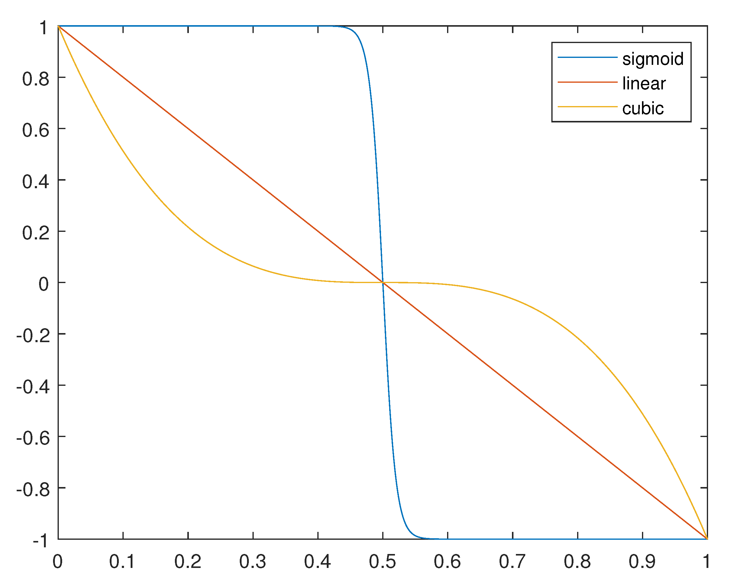
For the experiments, we will consider three mapping functions: a linear function (Equation (16a)); a sigmoid function (Equation (16b)); and a cubic function (Equation (16c)).
f mapping lin x : = 1 2 x ,
f mapping sig x : = 2 1 + e 100 1 2 x 1 ,
f mapping cub x : = 1 2 x 3 .
In Figure 6, we present the graph of all mappings defined in Equation (16). In all the cases, we can see that the range [ 0 , 1 ] is mapped origin-symmetrically to the range [ 1 , 1 ] .
We can easily see that the adaptive rules presented in our preliminary work [21] make up only a special case of the adaptation strategy through mapping functions discussed in this section.

5.8. Proposed Algorithm

The proposed method consists of the sequential use of all the operators discussed. As input, we must present the neighborhood matrix defined by the K sub-regions of a pre-segmented gray-level image I to the meta-heuristic. In this case, the following sequence of steps must be performed in order to obtain an artificial coloring with a high contrast set of colors for the image I:
Step 1
A population of chromosomes must be generated, each of which must be defined by K colors taken randomly in space Y ;
Step 2
Select individuals taking into account their fitness values for the crossover operator;
Step 3
Evaluate these individuals;
Step 4
Randomly select individuals to undergo mutation;
Step 5
Select the best individual among all those considered so far;
Step 6
Massively search its neighborhood for individuals with a better fitness value;
Step 7
Adjust the method parameters with the adaptation operator;
Step 8
Create a new population and evaluate it;
Step 9
If the maximum number of iterations has not been reached, then you need to go back to step 2.
This sequence of steps is detailed in the flowchart of the method, shown in Figure 7.

6. Experiments and Results

To evaluate the proposed methodology, we defined three distinct case studies (CS). In the first CS, we conduct a quantitative and a qualitative analysis of the proposed method considering a set of real world images. In the second CS, we compare the proposed method considering an extension of a well-established benchmark [54] of 24 synthetic and abstract unreal images in which its sub-regions are fully-connected. In the third CS, we conduct quantitative experiments considering the Munsell atlas color space. In addition, the experiments must confirm that the proposed method obtains the best performance in comparison with the current state-of-the-art techniques.

6.1. Setup and Implementation

The authors Radlak and Smolka [14] shared with us their GA code so that we could conduct computational analysis and comparisons fairly. In this way, our methodology is configured in order to keep the parameterization as similar as possible with their GA. In detail, we use as population size N pop = 30 ; the initial probabilities of mutation and crossover are defined as p mut = 0.1 and p × = 0.85 , respectively; half of the individuals selected to mutation operator must go through the subroutine Mut 1 and the other half must go through the subroutine Mut 2 , that is p LS = 0.5 ; the step-sizes η mut and η × from Equations (14) and (15), respectively, are both considered equals to 0.01 , in order to avoid abrupt changes in mutation and crossover rates; and the method runs for 10 4 iterations (generations). The computational experiments were performed at MATLAB environment on an i5-4460 PC with 8GB of ram.

6.2. Case Study I: Qualitative and Quantitative Analysis Considering Real World Images and Y = s R G B

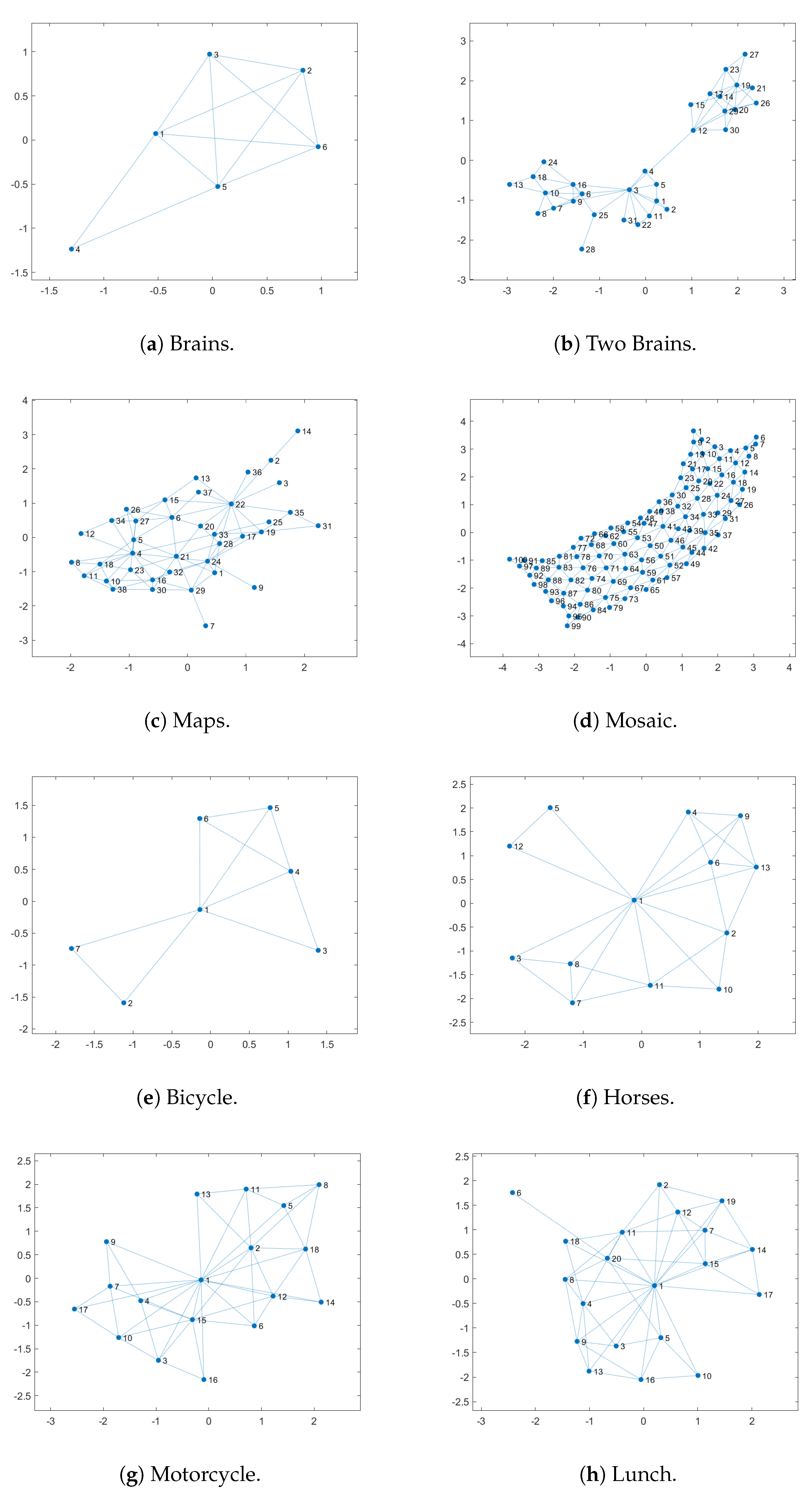
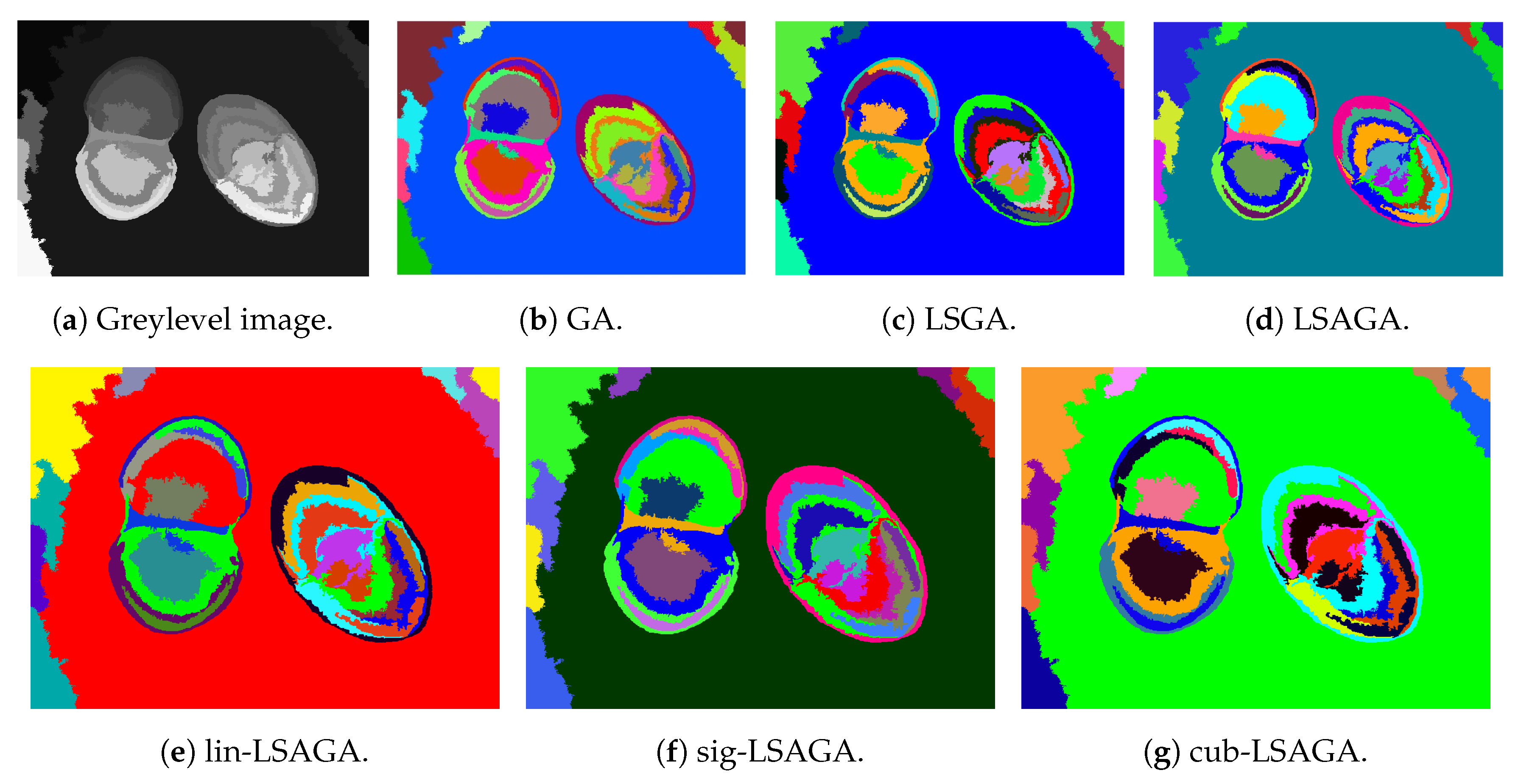
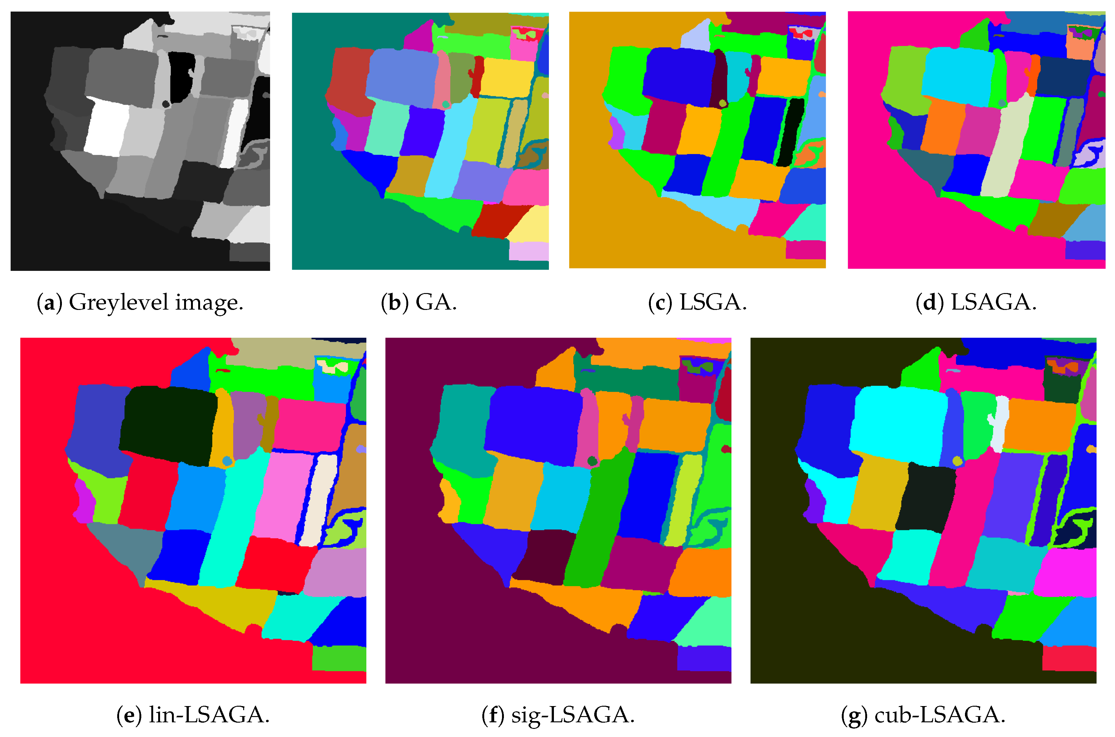
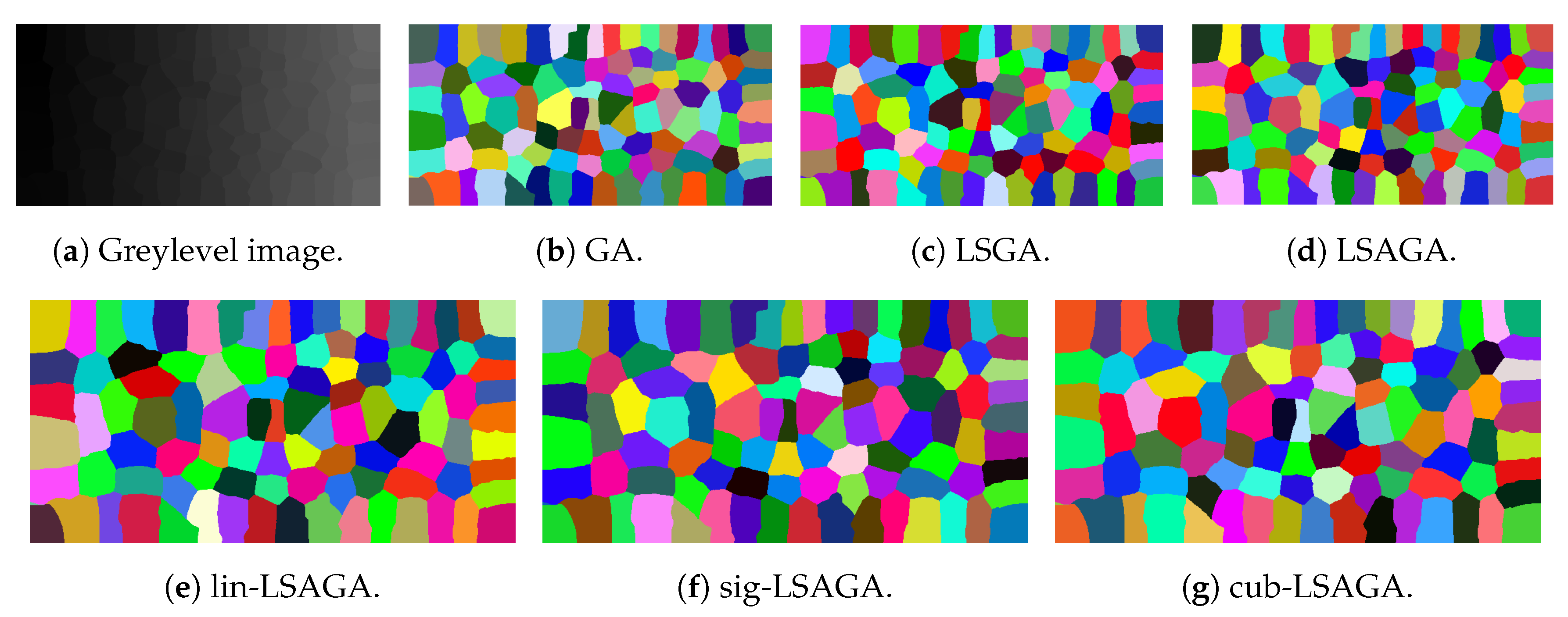
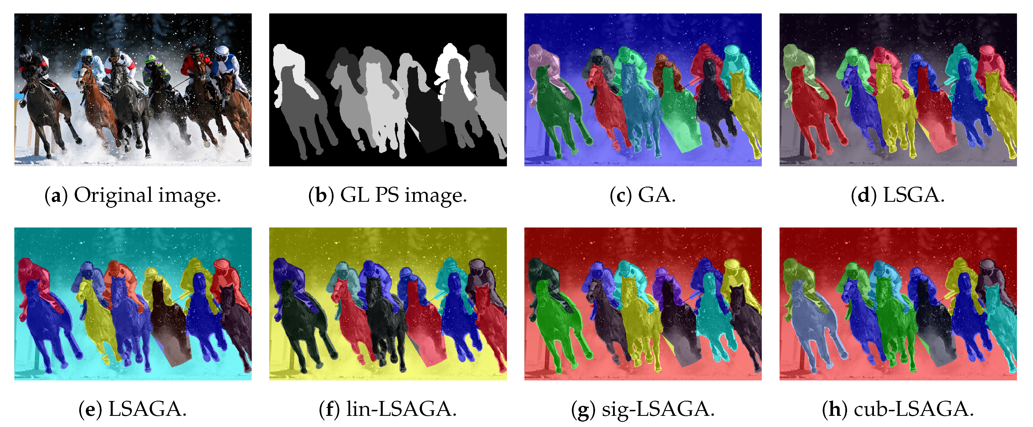
In this case study, we intend to evaluate the performance of the developed material taking into account the sRGB color space. That is, the PsCP solution defined by each image must be into Y = sRGB . For this, the proposed technique is evaluated on a set of eight images: four images used for experiments in the work of Radlak and Smolka [14] and in our preliminary work [21]; and the pre-segmented grey-level version of four images of the public dataset presented in the Pascal VOC 2012 segmentation challenge [55,56]. In Table 1, we present some structural details about the considered images, such as: the number (K) of sub-regions ( I 1 , I 2 ,   , I K ) of the image; the number of nonzero values in the neighborhood matrix ( Δ ) of the image; and the number of connections on the graph defined by the neighborhood matrix. We also present in Figure 8 the graph that describes the connections between the sub-regions of each image considered for this CS. In detail, the presented images that make up the evaluation benchmark for this CS are: “Brains”, in Figure 9a; “Two Brains”, in Figure 10a; “Maps”, in Figure 11a; “Mosaic”, in Figure 12a; “Bicycle”, in Figure 13a (File name in VOC 2012 dataset: “2007_000129.png”); “Horses”, in Figure 14a (File name in VOC 2012 dataset: “2008_004892.png”); “Motorcycle”, in Figure 15a (File name in VOC 2012 dataset: “2007_005173.png”); and “Lunch”, in Figure 16a (File name in VOC 2012 dataset: “2011_003066.png”).
GA [14] was selected for comparison because it is the most recent method that was published in this field and it is the most similar approach of our proposed method. We also selected for comparison the material that were developed in our previous work [21]: a method without the addition of adaptive rules, entitled local search genetic algorithm (LSGA); and another method with the addition of basic adaptive rules, entitled local search adaptive genetic algorithm (LSAGA). In addition, we evaluated three different versions of our method using the adaptive rules described in Section 5.7: the lin-LSAGA, the sig-LSAGA and the cub-LSAGA. For this, we will evaluate the LSAGA considering in the adaptive operator, respectively, the functions f mapping lin · , · , f mapping sig · , · and f mapping cub · , · , defined in Equation (16), as the mapping function. In Table 2, we present a summary of the compared methods and some of its respective specifications.
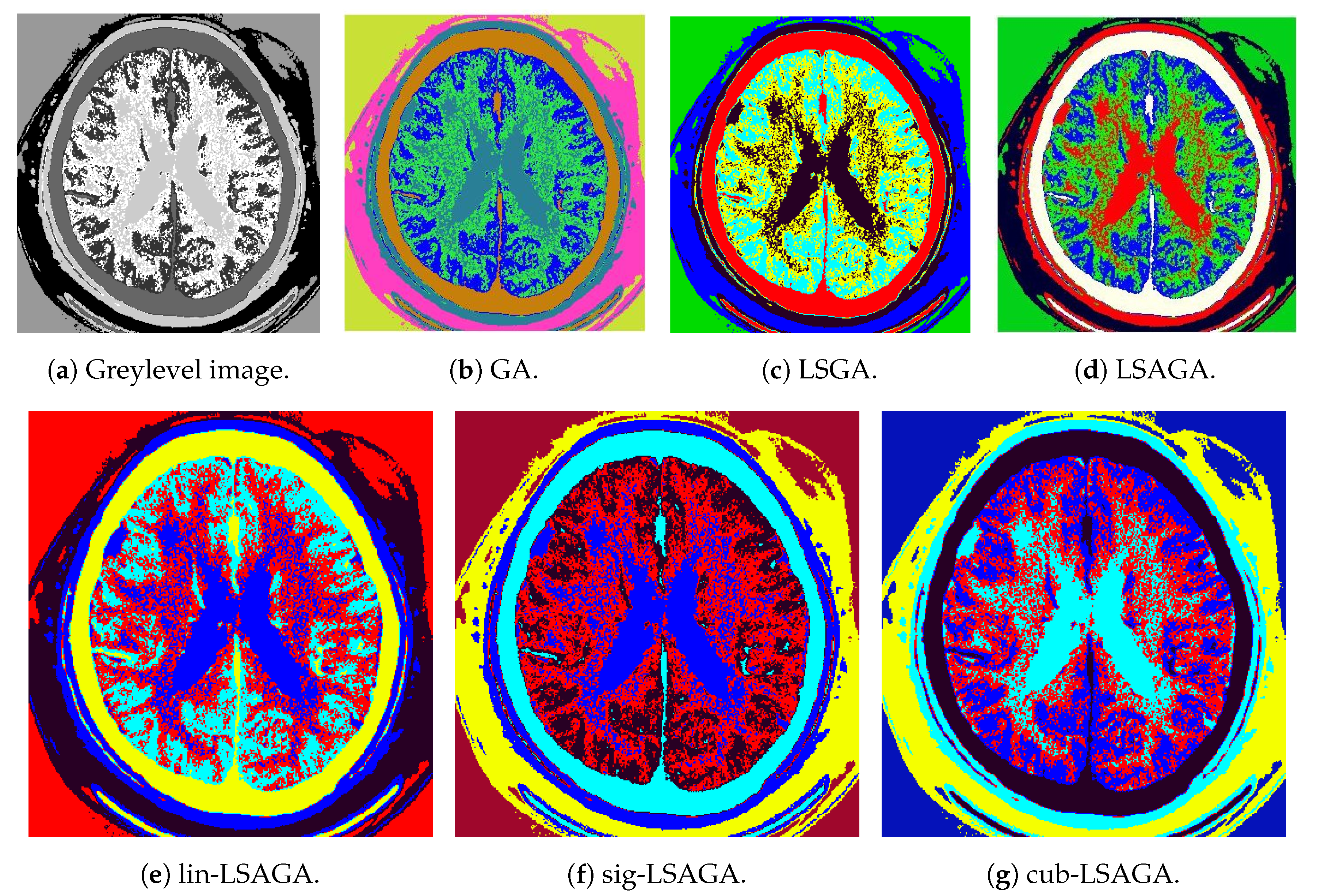
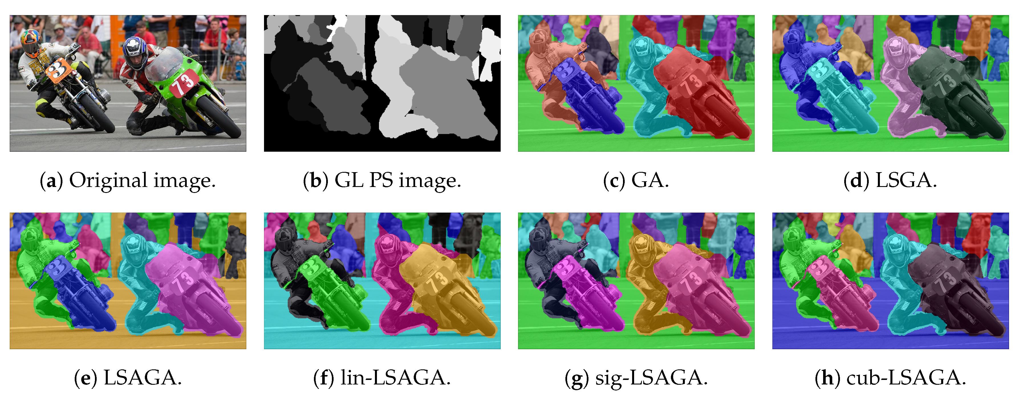
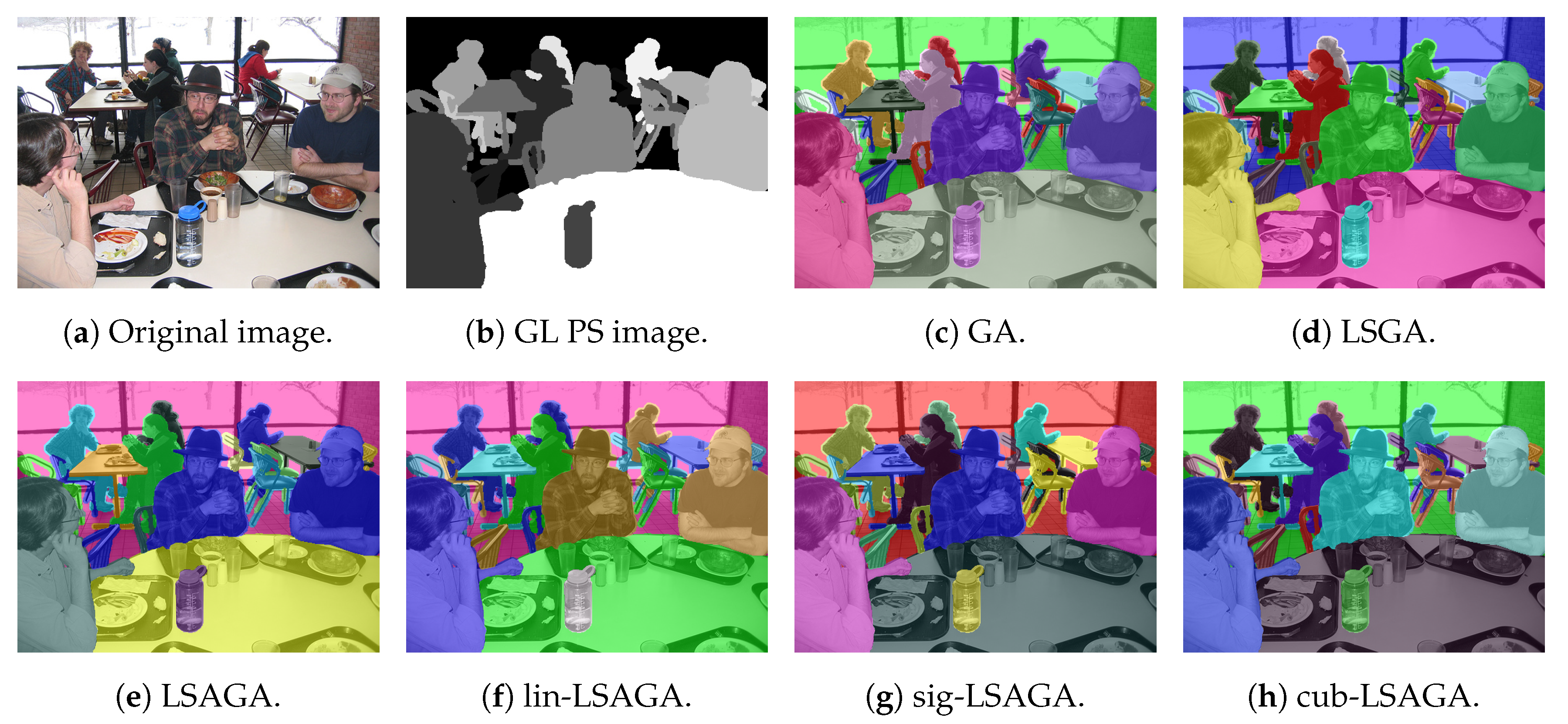
The best solution obtained for the PsCP using these techniques after 50 independent executions of each one, is shown in the Figure 9, Figure 10, Figure 11, Figure 12, Figure 13, Figure 14, Figure 15 and Figure 16, so that in Figure 9, Figure 10, Figure 11 and Figure 12 we present only the pseudo-colored pre-segmented image, while in Figure 13, Figure 14, Figure 15 and Figure 16 we present a fusion between the grey-level version of the original image with its pseudo-colored pre-segmented version.
Considering all the images in Figure 9, Figure 10, Figure 11, Figure 12, Figure 13, Figure 14, Figure 15 and Figure 16, we can see a evolution in the efficiency of visually detect a greater number of regions if we observe the image in greyscale and compare its respective pseudo-colored version. However, in some cases, one technique performs better than another. As highlighted in some examples in the sequence:
  • Brains: This image is not very complex, as it has only six sub-regions. However, we can see that, in the case of the pseudo-colorization obtained by GA (Figure 9b), the colors used in the central part of the brain are two different shades of green, which can cause some visual confusion. This does not occur with the pseudo-colorizations obtained by the other methods.
  • Two Brains: Concerning the images of the Two Brains, we can see that basic GA (Figure 10b) obtains a reasonably good visual separation between the sub-regions, presenting some confusion only with the colored regions in shades of red and pink in the central-left region of the image. In the pseudo-colorized image calculated by the LSGA method, there is also a confusion problem as well as in the basic GA. When analyzing Figure 10c, the central right region has a dark blue color very close to a region that was colored with black. These problems do not occur in the pseudo-colorization performed by the proposed technique with the addition of adaptive rules.
  • Maps: All methods used many shades of blue to pseudo-color this image, which can cause some visual confusion. For example, in the top-right section of the pseudo-colored image using the LSAGA technique (Figure 11d), we can see three colored regions with similar shades of blue. In addition, the pseudo-colored image with GA (Figure 11b) presents more serious issues. In detail, note that there is a small circular subregion in the right section of all pseudo-colored images, however, this subregion is almost visually imperceptible in the pseudo-colored image with GA.
  • Mosaic: That is an image in which the methods have great difficulty for pseudo-coloring due to their high number of sub-regions. However, even though all pseudo-colored images have a high degree of visual separability between their regions, it is possible to see that the pseudo-colorized version by GA (Figure 12b) has in its top-left part several shades of yellow in neighboring areas and has in its bottom-right section neighboring regions colored with similar shades of red and pink. Something similar also occurs with the pseudo-colorized image with the LSGA (Figure 12c).
  • Bicycle: The image has K = 6 sub-regions and a small number of connections are defined by the neighborhood matrix. Therefore, all techniques have good visual results. However, all images show shades of blue in some pair of neighboring sub-regions, but this does not compromise the visual distinction of each sub-region, since the shades of blue used are very dissimilar.
  • Horses: Analyzing the image, we can see that all methods present good pseudo-coloring results, with dissimilar color assignments in neighboring areas. However, this fact does not happen, for example, in the GA pseudo-colored image (Figure 14c), in which the blue horse in the central part of the image is pseudo-colored with a color visually similar to the background color.
  • Motorcycle: This image has a reasonably large number of sub-regions ( K = 18 ), yet all the techniques were able to associate a good pseudo-coloring for each sub-region, we highlight some negative points, such as in the case of the pseudo-colorized image by LSAGA (Figure 15e), which contains two people in the top-left part of the background that represent adjacent areas and that have been colored with shades visually similar in blue.
  • Lunch: That image is also highly complex, due to the number of sub-regions ( K = 20 ) that define a connection in the neighborhood matrix. Thus, not all techniques perform well. For example, in the pseudo-colorized image by our LSGA (Figure 16d), the table in the top-right part of the image receives a color similar to the background color. Something similar occurs with the color of the chair in the top-left section. Another example is presented by the pseudo-coloring obtained by our LSAGA (Figure 16e), which contains shades of blue in very close areas, such as the person in blue, in the central part of the image, sitting in a blue chair, in the case of the pseudo-colorized image by mapped methods this does not occur.
The numerical evaluations performed for this set of images confirm that the proposed methodology achieves superior performance. Table 3 shows a set of statistical values that were calculated using the fitness value obtained by each technique after 50 executions, in which the used measures are: the best presented fitness (Max); the worst presented fitness (Min); the mean value of the presented fitness (Mean); the standard deviation (STD); and the average time (AT) for each execution in seconds. In detail, we can see that the cub-LSAGA, the sig-LSAGA and the LSAGA methods find the best results in most images. Considering the nine images tested, cub-LSAGA found the best result in three images, sig-LSAGA found it in one image and LSAGA found it in five images. The methods that have an adaptation operator obtained the best results in the images, except for the Maps image that the best result was obtained by the LSGA method, however, the second-best value is presented by the sig-LSAGA, which is a method that also contains the mapped adaptive operator. In all the cases, a method that uses a mapped adaptive operator obtains the best Min value. In all images, the best statistical mean value was found by the methods that use the mapped adaptive operator. In addition, these same methods showed the smallest standard deviation in 7 of the 9 images considered, which shows that the methods proposed in this paper obtain more stable results when compared to other methods present in the literature, including our preliminary LSGA and LSAGA [21]. Analyzing the improvement of the results that were obtained by methods that make use of adaptive operator it is possible to verify that this operator has the capacity to guide LSGA and GA to find better solutions. However, GA is the method that obtained the lowest standard deviation in the case of the image “Mosaic”, which has a larger number of sub-regions. This fact occurred because the solutions obtained by GA are restricted to a lower set of fitness values, with the average values obtained by GA being around 25 units less than the average values obtained by our techniques in the image “Mosaic”.
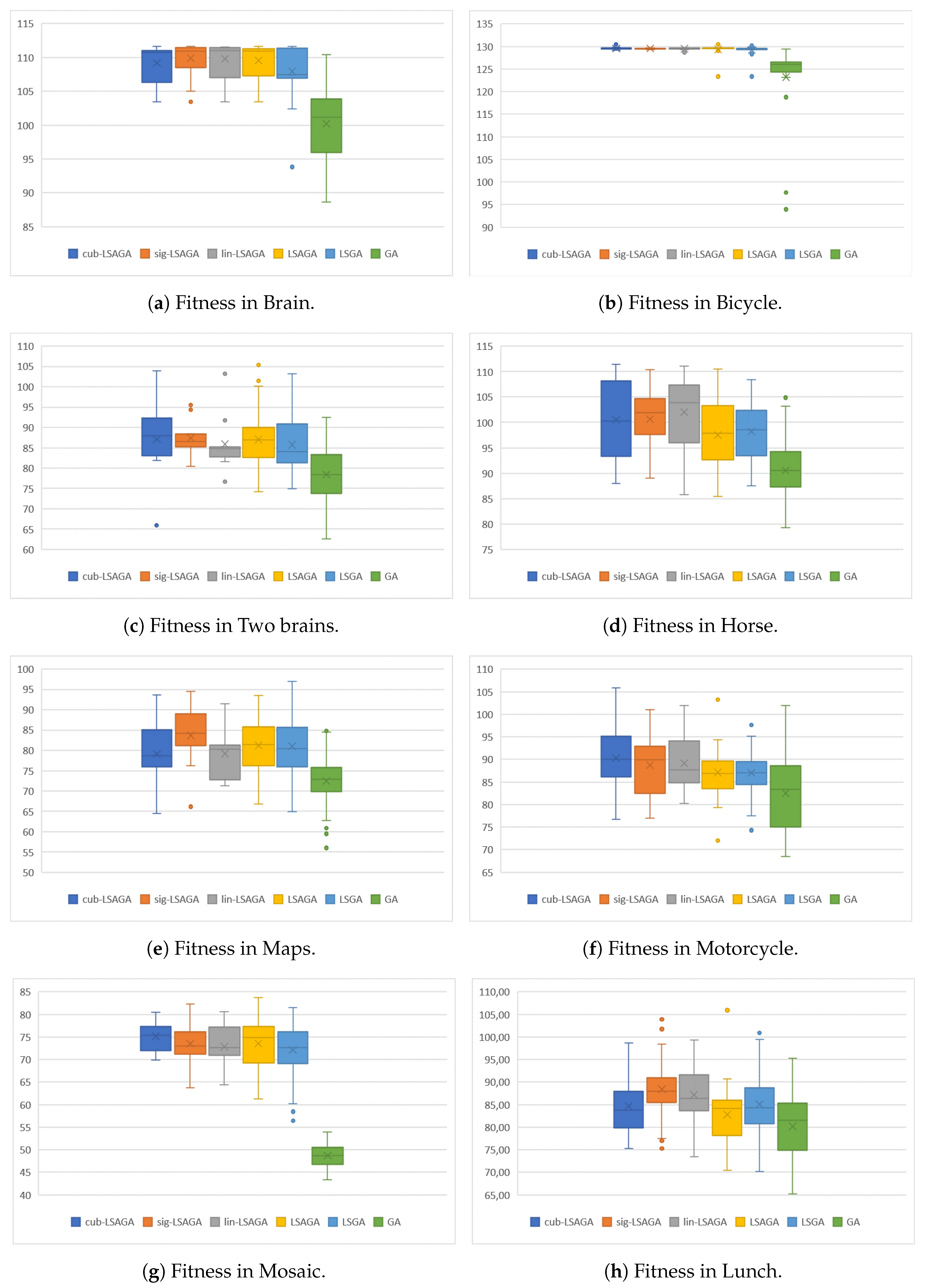
In Figure 17, a visual comparison of the performance of the techniques evaluated in the box plots is presented, so that we highlight information about the fitness values presented by the techniques during the 50 evaluations in each image that makes up the benchmark.
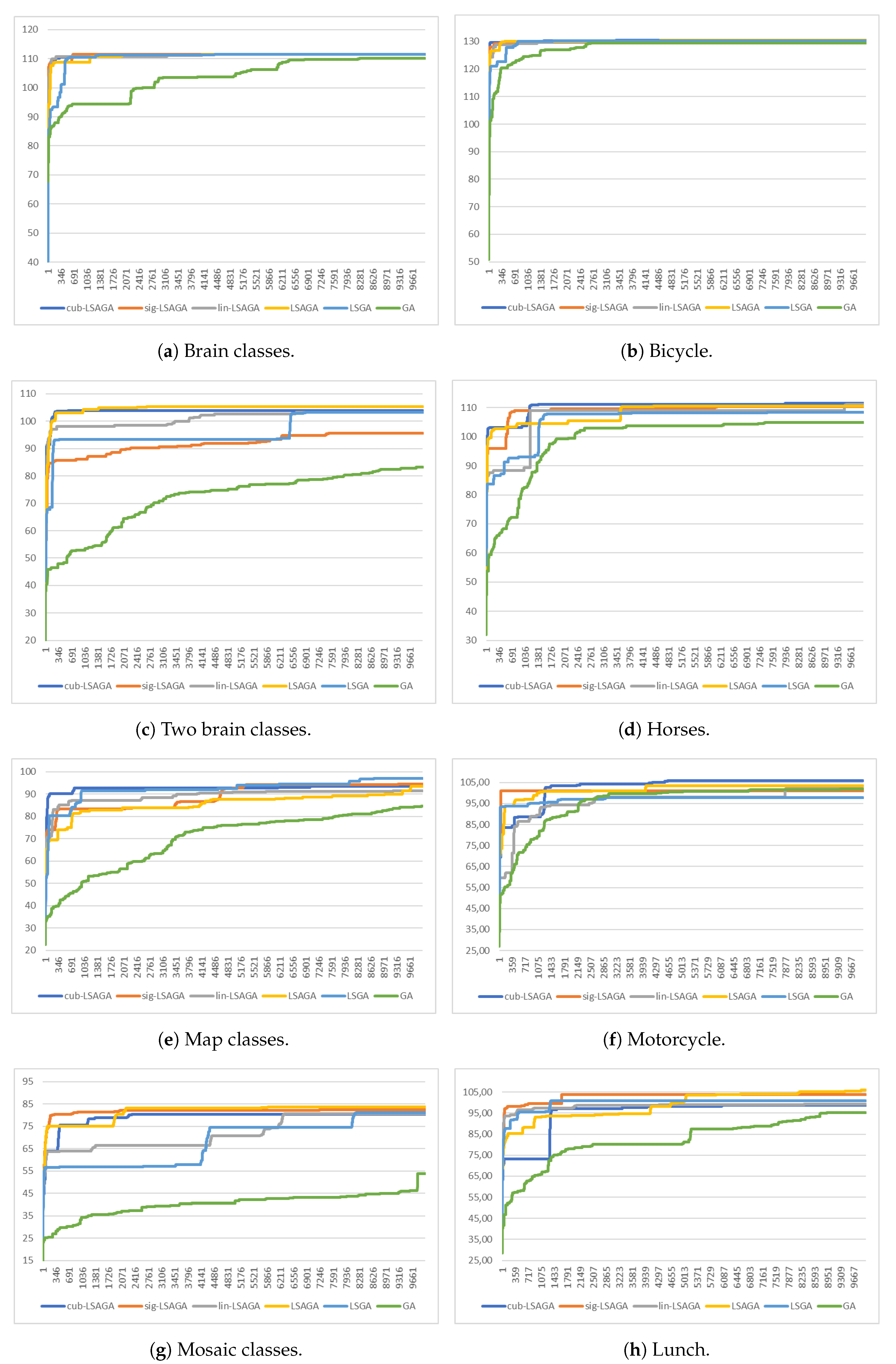
In images with a low number of regions, such as the image “Brains” which has K = 6 sub-regions and the image “Bicycle” which has K = 7 sub-regions, the proposed methodology presented a lower level of complexity and was able to obtain better results (Figure 17a) with less computational time, as shown in Table 3. This occurs because our methods do not create a parallel population for each color component of the RGB color space as the basic GA of Radlak and Smolka [14] does. If we observe cases where the number of regions increases, such as the cases of the images “Horses” ( K = 13 ), “Motorcycle” ( K = 18 ) and “Lunch” ( K = 20 ), the difference between GA computational time compared to our techniques decreases. It is clear that considering more complex images (Figure 17c,e,g), that is, images with a greater number of sub-regions, our methodology also obtains better numerical performance. However, the technique is more computationally costly compared to basic GA. This fact is due to the number of generations used, which, as we can analyze in the convergence curves presented in Figure 18, is a much larger number than necessary since our technique reaches the value equal to that obtained by GA or, at least, a very close value with less than 20% of the total number of iterations. This is an indication that our methodology could present the same performance with only 20 % of the total number of iterations used and, therefore, would consume only 20 % of the total time presented.
In this way, we conclude this CS noting that all the proposed techniques surpass basic GA in all the compared images. In addition, the mapped adaptive operators presented in this work produce more stable results in the RGB color space, in addition to producing pseudo-colorizations satisfactory to human vision. In contrast, computational time can be an opponent of our methodology in some situations, which must be circumvented by using more flexible configurations with fewer iterations.

6.3. Case Study II: Quantitative Analysis Considering a Synthetic Benchmark of Images and Y = s R G B

This second case study consists of evaluating the proposed techniques in 24 synthetic and abstract images, which are divided into fully-connected regions. In other words, this CS differs from the previous one in that we are going to evaluate the techniques in an extension of the Kelly [54] benchmark containing 24 images that do not necessarily exist in the real world. That is, in this CS, we are going to assume that we have available only the matrix of neighborhoods of a given grey-level image and execute the optimization methods on these matrices considering the Y as being the sRGB color space. Specifically, we will evaluate the methodology in images I K divided into K sub-regions I K , 1 , I K , 2 , , I K , K , such that the neighborhood matrix between these regions is in the form Δ K = ( δ i , j K ) i , j , with δ i , j K = 1 in the case of i j and δ i , j K = 0 otherwise, for K { 2 , 3 , , 25 } , as mathematically defined in Equation (17).
Δ K : = 1 K × K I K × K = 0 1 1 1 1 0 1 1 1 1 0 1 1 1 1 0 K × K ,
in which, 1 K × K is the K × K matrix with all the coordinates equals to 0, I K × K is the identity matrix with dimension K × K and K is the number of sub-regions considered for each case for K { 2 , 3 , , 25 } .
In this evaluation, we will take in comparison the same techniques considered in the previous CS (Table 2) with the same configuration used in CS I, and a Greedy Algorithm [14,36]. Table 4 shows the maximum fitness found for each technique between K colors, with K { 2 , 3 , , 25 } . All techniques were performed 50 times.
In this scenario, sig-LSAGA presented the best performance in 23 of the 24 images considered. The sig-LSAGA was the method that obtained the best results in the comparison. In addition, this technique did not present any worse results. Subsequently, our preliminary LSAGA method was the second method that presented the best values without presenting any worse value. Our lin-LSAGA method had the best result in 19 cases and the worst result in 2 cases; similar behavior to our cub-LSAGA, which had the best result in 18 cases and the worst result in 4 cases. These techniques present greater difficulties in images with more subregions (K larger). In addition, our LSGA technique presented the worst performance on only one occasion ( K = 4 ), unlike the Greedy Algorithm which presents the worst performance in simpler images ( 2 K 14 ) and the basic GA that presents the worst performance in more complex images ( 15 K 24 ). This fact demonstrates that the technology proposed in this work is robust in comparison to the other techniques, especially when we use adaptive rules since our methods showed the best results in all the synthetic images considered and numerically surpassing the values presented by the GA and Greedy Algorithm.

6.4. Case Study III: Quantitative Analysis Considering Real World Images and Y as Munsell Atlas Color Set

In this case study, we will evaluate our methodology on a set of real-world images, with the exception that we will consider Y to be the well-established Munsell color set [57] with 1269 colors, also known as Munsell atlas color set [58]. This set of colors is a perceptually uniform color space and, like the sRGB space, it is also defined by three components: hue, value and chroma [59].
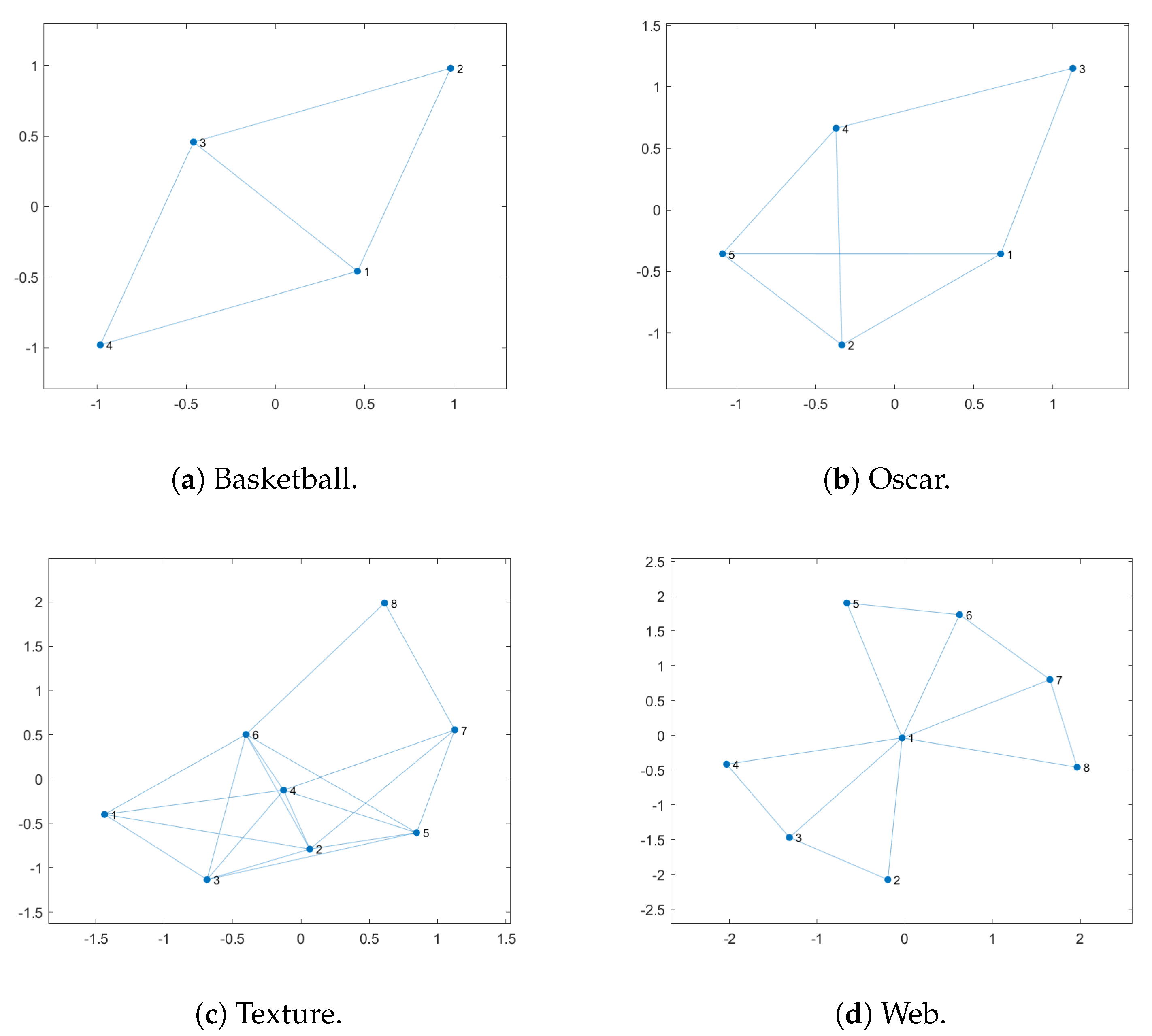
To the best of our knowledge, the most recent technique in the literature that evaluates this color space to obtain a high contrast set of colors is the local search (LS) technique by Bianco and Schettini [39]. The authors rate their methodology on a set of 5 real-world images. However, not all images used are available in the specialized literature. Therefore, to make the results reproducible, the authors make available the graphs that describe the neighborhood relationships between the subregions of each image. In this way, this CS, like the CS II, has only a quantitative assessment character, since we are not going to deal with the original images, but only with their neighborhood matrices. In this case, to conduct our analysis in this CS, we will consider all images used in [39] in which their sub-regions are connected by different graphs, totaling 4 out of 5. In this case, the images considered here are “Basketball”, “Texture”, “Oscar” and “Webpage”. The graph between the subregions of each of these images is represented in Figure 19. In addition, numerical details about these images can be viewed in Table 5.
For the evaluations of this case study, we will consider the same techniques considered in the previous case studies with the same configuration for each one. However, the basic GA compared in this situation is a version presented by Bianco and Schettini [39], which, according to the author, is an adaptation of the GA of Radlak and Smolka [14] to solve PsCP in Munsell’s color space. The authors also compare their methodology with a technique of randomly associating colors to images. Thus, we will also use the random association of colors for the sub-regions of the images for comparison, which is denoted by “Random”. This technique consists of randomly producing 1 , 000 , 000 possible color settings for each image and selecting the solution with the highest fitness value as a solution. Finally, we will present the values obtained by the Local Search (LS) technique of Bianco and Schettini [39]. In fact, the results of these last three techniques (GA, Random and LS) were collected directly from their original work. Whereas, our LSGA, LSAGA, lin-LSAGA, sig-LSAGA and cub-LSAGA techniques were executed 50 times independently of the configuration presented in the previous case studies. In Table 6, some statistical measures are presented regarding the 50 fitness values obtained by each of our techniques and their comparison with the results presented by the techniques discussed by Bianco and Schettini [39].
According to Table 6, the proposed methods show superior performance concerning most of the statistical measures considered. Below we highlight some details regarding each of the images in isolation:
  • Basketball: All the proposed methods have the same best value (Max) considering the 50 iterations. However, our cub-LSAGA method presents superior results considering the other statistical measures: worst value (Min), mean and standard deviation (STD). The LS method is deterministic and, therefore, presents the same solution in every evaluation. However, all of our methods have the worst values (Min), results higher than the result obtained by LS.
  • Texture: In this case, LS presents competitive results to our techniques. However, except for our cub-LSAGA, all the techniques proposed in this text have the best fitness value greater than the value obtained by LS. In addition, all techniques that make use of adaptation strategies presented a value of fitness as the worst value (Min), better than the best value presented by the Random technique. Likewise, our lin-LSAGA had the worst value greater than the best value presented by GA. This technique also presented the best average among all the compared techniques.
  • Oscar: In this case, except for cub-LSAGA, all of our techniques showed the highest best value. In addition, except for computational time, our sig-LSAGA presents the best statistical measures. It is worth mentioning that, all of the proposed techniques obtain a worse value for fitness than a better result than the other techniques with more than 10 units of difference.
  • Webpage: For this image, our sig-LSAGA presents the best fitness and average value. Meanwhile, our cub-LSAGA stands out considering the worst fitness value and the standard deviation. However, all the proposed techniques have higher average values than the best values presented by the other techniques.
In summary, we can see by observing Table 6 that our techniques surpass the results that make up the current state-of-the-art with special emphasis on the stability of techniques that use mapped adaptive operators. For example, considering the image “Basketball”, our cub-LSAGA, sig-LSAGA and lin-LSAGA methods showed standard deviations less than 1. In this case, our cub-LSAGA presented a standard deviation of 0.7331 . Something similar occurs in the image “Oscar”, in which our sig-LSAGA has a standard deviation of 0.9360 . Thus, this case study also confirms that the mapped adaptive methods proposed in this text help to maintain the stability of the method.
Regarding the average processing time of each technique, we realized that our methodology is, in fact, more computationally costly in all cases of this CS. Making our methodology used only in offline applications and it is not ideal to use it in applications that require real-time response. However, it presents superior results in comparison to the other techniques that define the state of the art.

7. Conclusions

In this paper, a new GA was proposed with the addition of specialized operators to reinforce the local search and with the addition of rules to adjust the parameters using symmetric mapping functions to treat the PsCP. All the steps contained in the proposed technique were presented in detail to facilitate the reproduction of the methodology.
We evaluated the proposed material in three case studies: in the first, our techniques were used to assign artificial coloring to real-world images and we performed qualitative and quantitative analyzes of the results obtained; in the second, our techniques were evaluated quantitatively in a benchmark of theoretical and synthetic images whose sub-regions are fully-connected; and in the third, we quantitatively evaluate our methodology when performing optimization in the Munsell color space. In the three case studies, the proposed methods obtained superior results when compared with other techniques presented in the state of the art. The proposed technique with the mapped adaptive rules presented the best results and it is the most stable version of our method. The combination of the inclusion of local search procedures and the use of more elaborate adaptive rules helped the method to obtain better results while maintaining a good genetic variability in the population and avoiding possible premature convergence.
In future works, we intend to expand the use of our mapped adaptation operators to update any GA configuration, such as the number of individuals in the population, the number of generations of the method, etc. In addition, we intend to study the effect that these strategies can have on other types of recent proposed meta-heuristics, such as the squirrel search algorithm [60], when applied to solve the PsCP. We believe that, even though the results obtained by the proposed method surpass the other state-of-the-art techniques, it is still necessary to conduct a study on techniques that can be used to reduce the computational time necessary to obtain the solutions to the problem, since if the image to be colored has a high number of sub-regions then the proposed method will need a very large amount of computational time to obtain good solutions. We also intend to use the proposed methodology to solve another class of problems in the literature, such as visual threat detection in X-ray scans [2,61].

Author Contributions

Conceptualization, M.S.V., O.M.J. and R.C.C.; methodology, M.S.V., O.M.J. and R.C.C.; software, M.S.V. and R.C.C.; validation, M.S.V. and R.C.C.; formal analysis, M.S.V. and R.C.C.; investigation, M.S.V. and R.C.C.; writing—original draft preparation, M.S.V. and R.C.C.; writing—review and editing, O.M.J.; visualization, R.C.C.; supervision, O.M.J.; project administration, O.M.J. All authors have read and agreed to the published version of the manuscript.

Funding

This study was financed in part by the Coordenação de Aperfeiçoamento de Pessoal de Nível Superior—Brasil (CAPES)—Finance Code 001, and by the São Paulo Research Foundation (FAPESP), process number 15/14358-0.

Acknowledgments

This study was financed in part by the Coordenação de Aperfeiçoamento de Pessoal de Nível Superior—Brasil (CAPES)—Finance Code 001, and by the São Paulo Research Foundation (FAPESP), process number 15/14358-0. We also thank the authors Radlak and Smolka [14] for sharing their GA code with us.

Conflicts of Interest

The authors declare no conflict of interest. The funders had no role in the design of the study; in the collection, analyses, or interpretation of data; in the writing of the manuscript, or in the decision to publish the results.

References

  1. Anitha, U.; Malarkkan, S.; Premalatha, J.; Manonmani, V. Comparison of standard edge detection techniques along with morphological processing and pseudo coloring in sonar image. In Proceedings of the 2016 International Conference on Emerging Trends in Engineering, Technology and Science (ICETETS), Pudukkottai, India, 24–26 February 2016; pp. 1–4. [Google Scholar]
  2. Dmitruk, K.; Denkowski, M.; Mazur, M.; Mikołajczak, P. Sharpening filter for false color imaging of dual-energy X-ray scans. Signal Image Video Process. 2017, 11, 613–620. [Google Scholar] [CrossRef] [Green Version]
  3. Etehadtavakol, M.; Ng, E.Y. Color segmentation of breast thermograms: A comparative study. In Application of Infrared to Biomedical Sciences; Springer: Singapore, 2017; pp. 69–77. [Google Scholar]
  4. Semary, N.A. A proposed Hsv-Based Pseudo-Coloring Scheme For Enhancing Medical Images. Comput. Sci. Inf. Technol. 2018. [Google Scholar] [CrossRef]
  5. Pipatnoraseth, T.; Phognsuphap, S.; Wiratkapun, C.; Tanawongsuwan, R.; Sajjacholapunt, P.; Shimizu, I. Breast Microcalcification Visualization Using Pseudo-Color Image Processing. In Proceedings of the 2019 12th Biomedical Engineering International Conference (BMEiCON), Ubon Ratchathani, Thailand, 19–22 November 2019; pp. 1–5. [Google Scholar]
  6. Zeng, X.; Tong, S.; Lu, Y.; Xu, L.; Huang, Z. Adaptive Medical Image Deep Color Perception Algorithm. IEEE Access 2020, 8, 56559–56571. [Google Scholar] [CrossRef]
  7. Pablo, R.; Verstraelen, P.; Simona, T.; Muthukumar, G.; Marzia, P.; Isabel, P.; Nathalie, C.; De Miguel-Pérez, D.; Riccardo, A.; Bals, S.; et al. Improving extracellular vesicles visualization: From static to motion. Sci. Rep. 2020, 10, 1–9. [Google Scholar]
  8. Wu, M.; Jin, X.; Jiang, Q.; Lee, S.; Guo, L.; Di, Y.; Huang, S.; Huang, J. Remote Sensing Image Colorization Based on Multiscale SEnet GAN. In Proceedings of the 2019 12th International Congress on Image and Signal Processing, BioMedical Engineering and Informatics (CISP-BMEI), Huaqiao, China, 19–21 October 2019; pp. 1–6. [Google Scholar]
  9. Beauchemin, M. Unsupervised colour coding for visualization of categorical maps. Remot. Sens. Lett. 2019, 10, 77–85. [Google Scholar] [CrossRef]
  10. Zheng, P.; Zhang, J. Quantitative nondestructive testing of wire rope based on pseudo-color image enhancement technology. Nondestruct. Test. Eval. 2019, 34, 221–242. [Google Scholar] [CrossRef]
  11. Burger, P.; Gillies, D. Interactive Computer Graphics: Functional, Procedural and Device-Level Methods; Addison-Wesley: Boston, MA, USA, 1989. [Google Scholar]
  12. Moodley, K.; Murrell, H. A colour-map plugin for the open source, Java based, image processing package, ImageJ. Comput. Geosci. 2004, 30, 609–618. [Google Scholar] [CrossRef]
  13. Carter, R.C.; Carter, E.C. High-contrast sets of colors. Appl. Opt. 1982, 21, 2936–2939. [Google Scholar] [CrossRef]
  14. Radlak, K.; Smolka, B. Visualization enhancement of segmented images using genetic algorithm. In Proceedings of the 2014 International Conference on Multimedia Computing and Systems (ICMCS), Marrakech, Morocco, 14–16 April 2014; pp. 391–396. [Google Scholar]
  15. Zang, W.; Ren, L.; Zhang, W.; Liu, X. A cloud model based DNA genetic algorithm for numerical optimization problems. Future Gener. Comput. Syst. 2018, 81, 465–477. [Google Scholar] [CrossRef]
  16. Asadzadeh, L. A local search genetic algorithm for the job shop scheduling problem with intelligent agents. Comput. Ind. Eng. 2015, 85, 376–383. [Google Scholar] [CrossRef]
  17. Lin, C. An adaptive genetic algorithm based on population diversity strategy. In Proceedings of the 2009 Third International Conference on Genetic and Evolutionary Computing, Guilin, China, 14–17 October 2009; pp. 93–96. [Google Scholar]
  18. Shojaedini, E.; Majd, M.; Safabakhsh, R. Novel adaptive genetic algorithm sample consensus. Appl. Soft Comput. 2019, 77, 635–642. [Google Scholar] [CrossRef] [Green Version]
  19. Zhu, K.Q. A diversity-controlling adaptive genetic algorithm for the vehicle routing problem with time windows. In Proceedings of the 15th IEEE International Conference on Tools with Artificial Intelligence, Sacramento, CA, USA, 3–5 November 2003; pp. 176–183. [Google Scholar]
  20. Xing, Y.; Chen, Z.; Sun, J.; Hu, L. An improved adaptive genetic algorithm for job-shop scheduling problem. In Proceedings of the Third International Conference on Natural Computation (ICNC 2007), Haikou, China, 24–27 August 2007; pp. 287–291. [Google Scholar]
  21. Contreras, R.C.; Morandin Junior, O.; Viana, M.S. A New Local Search Adaptive Genetic Algorithm for the Pseudo-Coloring Problem. In Advances in Swarm Intelligence; Tan, Y., Shi, Y., Tuba, M., Eds.; Springer International Publishing: Cham, Switzerland, 2020; pp. 349–361. [Google Scholar]
  22. Appel, K.I.; Haken, W. Every Planar Map is Four Colorable; American Mathematical Soc.: Providence, RI, USA, 1989; Volume 98. [Google Scholar]
  23. Jensen, T.R.; Toft, B. Graph Coloring Problems; John Wiley & Sons: New York, NY, USA, 2011; Volume 39. [Google Scholar]
  24. Christensen, J.; Shieber, S.M.; Marks, J. Placing Text Labels on Maps and Diagrams; Academic Press: Cambridge, MA, USA, 1994. [Google Scholar]
  25. Welsh, T.; Ashikhmin, M.; Mueller, K. Transferring Color to Greyscale Images. In Proceedings of the 29th Annual Conference on Computer Graphics and Interactive Techniques, San Antonio, TX, USA, 23–26 July 2002. [Google Scholar]
  26. Zare, M.; Lari, K.B.; Jampour, M.; Shamsinejad, P. Multi-GANs and its application for Pseudo-Coloring. In Proceedings of the 2019 4th International Conference on Pattern Recognition and Image Analysis (IPRIA), Tehran, Iran, 6–7 March 2019; pp. 1–6. [Google Scholar]
  27. Fang, F.; Wang, T.; Zeng, T.; Zhang, G. A Superpixel-based Variational Model for Image Colorization. IEEE Trans. Vis. Comput. Graph. 2019, 26, 2931–2943. [Google Scholar] [CrossRef] [PubMed]
  28. Wan, S.; Xia, Y.; Qi, L.; Yang, Y.; Atiquzzaman, M. Automated Colorization of a Grayscale Image With Seed Points Propagation. IEEE Trans. Multimed. 2020, 22, 1756–1768. [Google Scholar] [CrossRef]
  29. Li, B.; Lai, Y.K.; Rosin, P.L. A review of image colourisation. In Handbook Of Pattern Recognition And Computer Vision; World Scientific: Singapore, 2020; p. 139. [Google Scholar]
  30. Dai, J.; Zhou, S. Computer-aided pseudocolor coding of gray images: Complementary color-coding technique. In Electronic Imaging and Multimedia Systems; Li, C.S., Stevenson, R.L., Zhou, L., Eds.; International Society for Optics and Photonics (SPIE): Beijing, China, 1996; Volume 2898, pp. 186–191. [Google Scholar]
  31. Campadelli, P.; Mora, P.; Schettini, R. Color set selection for nominal coding by Hopfield networks. Vis. Comput. 1995, 11, 150–155. [Google Scholar] [CrossRef]
  32. Green-Armytage, P. A colour alphabet and the limits of colour coding. JAIC J. Int. Colour Assoc. 2010, 5, 1–23. [Google Scholar]
  33. Campadelli, P.; Posenato, R.; Schettini, R. An algorithm for the selection of high-contrast color sets. Color Res. Appl. 1999, 24, 132–138. [Google Scholar] [CrossRef]
  34. Brill, M.H.; Robertson, A.R.; Schanda, J. Open problems on the validity of Grassmann’s laws. Color. Underst. Cie Syst. 2007, 245–259. [Google Scholar]
  35. Glasbey, C.; van der Heijden, G.; Toh, V.F.; Gray, A. Colour displays for categorical images. Color Res. Appl. 2007, 32, 304–309. [Google Scholar] [CrossRef] [Green Version]
  36. Bianco, S.; Citrolo, A.G. High Contrast Color Sets under Multiple Illuminants. In Computational Color Imaging; Tominaga, S., Schettini, R., Trémeau, A., Eds.; Springer: Berlin/Heidelberg, Germany, 2013; pp. 133–142. [Google Scholar]
  37. Kirkpatrick, S.; Gelatt, C.D.; Vecchi, M.P. Optimization by simulated annealing. Science 1983, 220, 671–680. [Google Scholar] [CrossRef]
  38. Holland, J.H. Adaptation in Natural and Artificial Systems: An Introductory Analysis with Applications to Biology, Control, and Artificial Intelligence; MIT Press: Cambridge, MA, USA, 1992. [Google Scholar]
  39. Bianco, S.; Schettini, R. Unsupervised color coding for visualizing image classification results. Inf. Vis. 2018, 17, 161–177. [Google Scholar] [CrossRef]
  40. Connolly, C.; Fleiss, T. A study of efficiency and accuracy in the transformation from RGB to CIELAB color space. IEEE Trans. Image Process. 1997, 6, 1046–1048. [Google Scholar] [CrossRef]
  41. Mahyar, F.; Cheung, V.; Westland, S.; Henry, P. Investigation of complementary colour harmony in CIELAB colour space. In Proceedings of the AIC Midterm Meeting, Hangzhou, China, 12–14 July 2007. [Google Scholar]
  42. Hoeser, T.; Kuenzer, C. Object Detection and Image Segmentation with Deep Learning on Earth Observation Data: A Review-Part I: Evolution and Recent Trends. Remot. Sens. 2020, 12, 1667. [Google Scholar] [CrossRef]
  43. Pare, S.; Kumar, A.; Singh, G.; Bajaj, V. Image segmentation using multilevel thresholding: A research review. Iran. J. Sci. Technol. Trans. Electr. Eng. 2020, 44, 1–29. [Google Scholar] [CrossRef]
  44. Taghanaki, S.A.; Abhishek, K.; Cohen, J.P.; Cohen-Adad, J.; Hamarneh, G. Deep semantic segmentation of natural and medical images: A review. Artif. Intell. Rev. 2020, 14, 1–42. [Google Scholar] [CrossRef]
  45. Viana, M.S.; Morandin Junior, O.; Contreras, R.C. A Modified Genetic Algorithm With Local Search Strategies And Multi-Crossover Operator For Job Shop Scheduling Problem. Sensors 2020, 20, 5440. [Google Scholar] [CrossRef]
  46. Zames, G.; Ajlouni, N.; Holland, J.; Hills, W.; Goldberg, D. Genetic algorithms in search, optimization and machine learning. Inf. Technol. J. 1981, 3, 301–302. [Google Scholar]
  47. Goldberg, D.E. Genetic algorithms in search. Optim. Mach. 1989, 1. [Google Scholar]
  48. Dioşan, L.; Oltean, M. Evolving crossover operators for function optimization. In European Conference on Genetic Programming; Springer: Berlin/Heidelberg, Germany, 2006; pp. 97–108. [Google Scholar]
  49. Ombuki, B.M.; Ventresca, M. Local search genetic algorithms for the job shop scheduling problem. Appl. Intell. 2004, 21, 99–109. [Google Scholar] [CrossRef]
  50. Amjad, M.K.; Butt, S.I.; Kousar, R.; Ahmad, R.; Agha, M.H.; Faping, Z.; Anjum, N.; Asgher, U. Recent research trends in genetic algorithm based flexible job shop scheduling problems. Math. Probl. Eng. 2018, 2018. [Google Scholar] [CrossRef] [Green Version]
  51. Bäck, T.; Schwefel, H.P. An overview of evolutionary algorithms for parameter optimization. Evol. Comput. 1993, 1, 1–23. [Google Scholar] [CrossRef]
  52. Hinterding, R. Gaussian mutation and self-adaption for numeric genetic algorithms. In Proceedings of the 1995 IEEE International Conference on Evolutionary Computation, Perth, Australia, 29 November–1 December 1995; p. 384. [Google Scholar]
  53. Bulmer, M.G. Principles of Statistics; Courier Corporation: New York, NY, USA, 1979. [Google Scholar]
  54. Kelly, K.L. Twenty-two colors of maximum contrast. Color Eng. 1965, 3, 26–27. [Google Scholar]
  55. Everingham, M.; Winn, J. The pascal visual object classes challenge 2012 (voc2012) development kit. Pattern Anal. Stat. Model. Comput. Learn. Tech. Rep. 2011, 8, 1–32. [Google Scholar]
  56. Everingham, M.; Eslami, S.A.; Van Gool, L.; Williams, C.K.; Winn, J.; Zisserman, A. The pascal visual object classes challenge: A retrospective. Int. J. Comput. Vis. 2015, 111, 98–136. [Google Scholar] [CrossRef]
  57. Newhall, S.M.; Nickerson, D.; Judd, D.B. Final report of the OSA subcommittee on the spacing of the Munsell colors. JOSA 1943, 33, 385–418. [Google Scholar] [CrossRef]
  58. Munsell, A.H. Munsell Book of Color: Matte Finish Collection; Munsell Color: Baltimore, MD, USA, 1992. [Google Scholar]
  59. Campadelli, P.; Schettini, R.; Zuffi, S. A system for the automatic selection of conspicuous color sets for qualitative data display. IEEE Trans. Geosci. Remot. Sens. 2001, 39, 2283–2286. [Google Scholar] [CrossRef]
  60. Jain, M.; Singh, V.; Rani, A. A novel nature-inspired algorithm for optimization: Squirrel search algorithm. Swarm Evol. Comput. 2019, 44, 148–175. [Google Scholar] [CrossRef]
  61. Xue, Z.; Blum, R.S. Concealed weapon detection using color image fusion. In Proceedings of the 6th International Conference on Information Fusion, Cairns, Queensland, Australia, 8–11 July 2003; pp. 622–627. [Google Scholar]
Publisher’s Note: MDPI stays neutral with regard to jurisdictional claims in published maps and institutional affiliations.
Figure 1. A grey-level image I; its sub-regions I 1 , I 2 , I 3 and I 4 ; the graph representing the connections between the sub-regions; and its associated neighborhood matrix Δ .
Symmetry 12 01684 g001
Figure 2. Pipeline of the proposed methodology for solve the pseudo-coloring problem (PsCP).
Symmetry 12 01684 g002
Figure 3. Example of pseudo-coloring of a grey-level image I, pre-segmented in K = 4 regions, according to a chromosome C in the color space Y = sRGB.
Symmetry 12 01684 g003
Figure 4. Schematic of the proposed crossover operator. Such that α i is a random value taken in [ 0 , 1 ] for all i.
Symmetry 12 01684 g004
Figure 5. Schematic diagram of the functioning of three mutation functions on the same chromosome C .
Symmetry 12 01684 g005
Figure 6. The plot of the graph of the mapping functions considered for the proposed mapped adaptive operator.
Symmetry 12 01684 g006
Figure 7. Flow chart of our proposed mapped local search adaptive genetic algorithm.
Symmetry 12 01684 g007
Figure 8. Graph of the neighborhood matrix between the sub-regions of each grey-level image. The number in each node is the associated index of the sub-region.
Symmetry 12 01684 g008
Figure 9. Pseudo-colored results for the grey-level image “Brain”.
Symmetry 12 01684 g009
Figure 10. Pseudo-colored results for the grey-level image “Two Brains”.
Symmetry 12 01684 g010
Figure 11. Pseudo-colored results for the grey-level image “Maps”.
Symmetry 12 01684 g011
Figure 12. Pseudo-colored results for the grey-level image “Mosaic”.
Symmetry 12 01684 g012
Figure 13. Pseudo-colored results for the grey-level image “Bicycle”.
Symmetry 12 01684 g013
Figure 14. Pseudo-colored results for the grey-level image “Horses”.
Symmetry 12 01684 g014
Figure 15. Pseudo-colored results for the grey-level image “Motorcycle”.
Symmetry 12 01684 g015
Figure 16. Pseudo-colored results for the grey-level image “Lunch”.
Symmetry 12 01684 g016
Figure 17. Numerical results (fitness values) displayed in boxplots of 50 independent runs of each technique.
Symmetry 12 01684 g017
Figure 18. Convergence analysis.
Symmetry 12 01684 g018
Figure 19. Graph of the neighborhood matrix between the sub-regions of each grey-level image used in the work of Bianco and Schettini [39]
Symmetry 12 01684 g019
Table 1. Structural details about the used images.
ImageNumber of Subregions (K)Nonzero Values in Δ Number of Connections in the Graph
Brains62412
Two Brains3113266
Maps3817487
Mosaic100502251
Bicycle72211
Horses135829
Motorcycle189648
Lunch2011055
Table 2. Methods used for comparison. The symbol “-” means that the method does not use a mapping function.
MethodLocal SearchSimple Adaptive RulesMapped Adaptive RulesMapping Function
GANoNoNo-
LSGAYesNoNo-
LSAGAYesYesNo-
lin-LSAGAYesNoYesYes (Equation (16a))
sig-LSAGAYesNoYesYes (Equation (16b))
cub-LSAGAYesNoYesYes (Equation (16c))
Table 3. Statistical measurements of the fitness values presented in 50 runs of each method for the case study (CS) I images. The values highlighted in bold represent the best value of the evaluated measure available in the line.
Cub-LSAGASig-LSAGALin-LSAGALSAGALSGAGA
ImageBrain
Max111.5897111.5897111.5685111.5897111.5897110.4434
Min103.4240103.4240103.4240103.424093.815988.6637
Mean109.2113109.9077109.7841109.5214107.9427100.2385
STD2.92572.30712.41982.35633.93055.2523
AT (s)39.959946.440145.114244.496533.958466.9531
ImageTwo Brains
Max103.895095.5579103.2217105.3690103.243792.4752
Min65.864580.435476.606674.193474.927762.6070
Mean87.092087.415685.884687.038985.715778.3665
STD9.47224.37496.85716.22916.91726.9151
AT (s)160.4555157.1275163.7412158.64375144.095997.7062
ImageMaps
Max93.705494.556491.475793.539997.067685.1661
Min64.465666.147571.250766.866264.936055.9863
Mean79.116383.682379.216381.225880.992272.4412
STD8.09987.64336.15626.64156.46026.2322
AT (s)222.9510226.4532226.4238224.1458203.8438130.4597
ImageMosaic
Max80.483882.289580.639283.788081.513353.8912
Min69.877363.750064.442761.270656.416843.3865
Mean75.183373.534272.835673.559172.115548.7392
STD3.42944.92395.18496.28695.77672.4751
AT (s)990.0295992.4713991.2589989.3925936.8443331.4825
ImageBicycle
Max130.4377129.6426129.6426130.5154130.2436129.3809
Min129.1017129.3329128.6836123.3457123.345793.9292
Mean129.5630129.5257129.4862129.3585129.2352123.2097
STD0.24390.12190.20941.26291.26068.5688
AT (s)40.354142.489648.498445.578134.057368.9844
ImageHorse
Max111.4548110.3349111.0386110.5609108.4003104.8786
Min87.977089.008585.798785.384587.488379.3059
Mean100.5157100.6137102.027097.474798.198190.5370
STD7.61745.68106.57077.27565.85456.0897
AT (s)72.554773.941275.249669.130253.572974.4583
ImageMotorcycle
Max105.8383101.0411101.9775103.530997.8846101.8992
Min76.773377.000480.205772.046974.310168.4586
Mean90.322388.740389.155387.093987.066082.5259
STD7.14766.46536.15156.64376.07118.9604
AT (s)89.741285.921486.664789.656373.505285.3021
ImageLunch
Max98.6577103.884899.3338105.9357100.896795.3289
Min75.295075.267773.463970.4378670.148165.2178
Mean84.707688.426887.156982.8168185.089380.1618
STD6.02117.34646.13057.35617.28667.7565
AT (s)103.249799.146398.8976100.817782.447987.6302
Table 4. Max distance of colors in a fully-connected images. Green numbers are the max (best) values in line and red numbers are the min (worst) values in line.
Regions (K)Cub-LSAGASig-LSAGALin-LSAGALSAGALSGAGA [14]Greedy [14]
2249.2249.2249.2249.2249.2249.2233.85
3166.11166.11166.11166.11166.11166.11164.64
4130.64130.64130.64130.64129.64130.21129.64
5111.59111.59111.59111.59111.59111.43108.81
6102.58102.58102.58102.58102.58102.4893.78
794.794.794.794.793.7593.0486.95
886.1586.1586.1586.1586.1384.7880.03
981.4981.4981.4981.4980.4378.6874.45
1077.877.877.877.874.974.6571.92
1168.169.4369.4369.4368.166.7165.77
1265.6165.6165.6165.6164.6564.8461.86
1364.2664.2664.2664.2662.563.1357.79
1460.8960.8960.8960.8959.158.857.32
1557.1657.1657.1657.1656.753.5255.27
1651.5355.8255.8255.8251.5351.0153.4
1753.5653.5653.5653.5652.5549.6751.32
1850.5650.5650.5650.5650.4748.1749.42
1945.0850.547.950.548.2445.0847.9
2044.6749.2649.2649.2645.8344.6747.57
2146.5445.6845.6845.6844.7842.6646.54
2246.3646.3644.2346.3644.8741.6344.23
2344.7444.7444.7443.6243.2841.344.74
2439.7743.8639.7743.8642.2239.7743.61
2538.5543.0938.5543.0941.8238.5541.98
Table 5. Details about the used images for the CS III.
ImageNumber of Subregions (K)Nonzero Values in Δ Number of Connections in the Graph
Basketball4105
Texture83819
Oscar5147
Webpage82412
Table 6. Optimization in Munsell Atlas color space with 1269 colors. The symbol “-” means that the respective measurement is not available in the original work. The values highlighted in bold represent the best value of the evaluated measure available in the table line.
Cub-LSAGASig-LSAGALin-LSAGALSAGALSGAGA [14,39]Random [39]LS [39]
ImageBasketball
Max83.819383.819383.819383.819383.819370.160.9570.1
Min80.920380.273380.920378.123974.6126---
Mean82.514082.205782.217982.035881.804861.6817.76-
STD0.73310.81820.75001.20271.4551---
AT (s)38.335440.400138.735239.656332.359415.080.00133.03
ImageTexture
Max58.746563.507563.065166.361263.065147.4545.1560.63
Min46.782346.083647.711445.812036.5557---
Mean53.073154.409555.438354.657052.430343.7517.78-
STD3.32794.07773.40214.63425.7014---
AT (s)58.120559.980159.255250.536535.822929.480.002118.87
ImageOscar
Max82.416583.819383.819383.819383.819359.7656.4463.5
Min78.123979.565278.123977.314876.4953---
Mean81.808182.060581.942081.783281.256854.7418.74-
STD1.31610.93601.07571.41101.6553---
AT (s)39.885442.146440.755239.000028.557317.930.00155.56
ImageWebpage
Max80.920382.374382.281182.170280.920350.1342.9362.33
Min67.243062.877464.409562.877462.2342---
Mean75.734276.915276.126376.065173.651144.1514.89-
STD4.08634.78454.62174.60635.5967---
AT (s)50.125447.894647.774048.666737.015630.360.00218.99