Article

Multi-Scale and Multi-Branch Convolutional Neural Network for Retinal Image Segmentation

College of Computer Science and Engineering, Northwest Normal University, Lanzhou 730070, China
*
Author to whom correspondence should be addressed.
These authors contributed equally to this work.
Symmetry 2021, 13(3), 365; https://doi.org/10.3390/sym13030365
Submission received: 6 January 2021 / Revised: 15 February 2021 / Accepted: 19 February 2021 / Published: 24 February 2021
(This article belongs to the Special Issue Symmetry in Vision II)

Abstract

:
The accurate segmentation of retinal images is a basic step in screening for retinopathy and glaucoma. Most existing retinal image segmentation methods have insufficient feature information extraction. They are susceptible to the impact of the lesion area and poor image quality, resulting in the poor recovery of contextual information. This also causes the segmentation results of the model to be noisy and low in accuracy. Therefore, this paper proposes a multi-scale and multi-branch convolutional neural network model (multi-scale and multi-branch network (MSMB-Net)) for retinal image segmentation. The model uses atrous convolution with different expansion rates and skip connections to reduce the loss of feature information. Receiving domains of different sizes captures global context information. The model fully integrates shallow and deep semantic information and retains rich spatial information. The network embeds an improved attention mechanism to obtain more detailed information, which can improve the accuracy of segmentation. Finally, the method of this paper was validated on the fundus vascular datasets, DRIVE, STARE and CHASE datasets, with accuracies/F1 of 0.9708/0.8320, 0.9753/0.8469 and 0.9767/0.8190, respectively. The effectiveness of the method in this paper was further validated on the optic disc visual cup DRISHTI-GS1 dataset with an accuracy/F1 of 0.9985/0.9770. Experimental results show that, compared with existing retinal image segmentation methods, our proposed method has good segmentation performance in all four benchmark tests.

1. Introduction

Retina image detection assists ophthalmologists in diagnosing different eye diseases, such as diabetic retinopathy, glaucoma, age-related macular degeneration and other diseases [1], among which diabetic retinopathy is the main cause of blindness. The condition of retinal blood vessels (slope, curvature, neovascularization, etc.) is an important indicator for diagnosing retinal diseases. The fundus image structure of the diseased retina includes microaneurysms, hemorrhage and exudates, etc. [2], referring to Figure 1b. In clinical testing of glaucoma, the vertical cup-to-disk ratio (CDR) is usually calculated to diagnose whether it is glaucoma [3]. CDR is the vertical cup diameter (VCD) divided by the vertical disk diameter (VDD). The normal CDR range is from 0.3 to 0.4. If the CDR is larger, it may indicate glaucoma or other ophthalmic neurological diseases, referring to Figure 1c,d.
Manual detection of ocular diseases is usually a challenging and time-consuming task for ophthalmologists. The accurate acquisition of information in retinal images is used to assist ophthalmologists in detecting ocular diseases. Currently, a large number of scholars have worked on retinal image tissue segmentation. Y. Miao et al. [4] proposed a retinal vessel extraction method using matched filtering and a local entropy threshold. Kundu et al. [5] proposed a retinal vessel segmentation method, which creates a proportional space from the perspective of morphology. Palomera-Perez et al. [6] proposed the segmentation of retinal vessels based on multi-scale feature extraction and region growth algorithms, but specialized knowledge is needed for the setting of vessel seed points and the formulation of termination rules. In [7,8,9], the B-COSFIRE filter, the Gabor wavelet and Gaussian filter response are proposed for retinal vessel segmentation. These traditional machine learning methods do not have a strong ability to learn features automatically compared to deep learning methods, and the segmentation accuracy is not high. Jainish et al. [10] proposed a retinal vessel extraction method based on the maximum entropy EM algorithm. The above literature uses an unsupervised method for the segmentation of retinal tissue. This method does not require reference to manual annotation and uses the default rules of blood vessels to specify the venous regions, since the unsupervised method suffers from the problems of not very good performance and generality caused by noise and pathological patterns.
In this paper, a supervised learning approach is adopted to solve this problem. Unlike the unsupervised approach, the supervised approach uses manually annotated data to train a complex classifier for segmentation. The literature [11] uses neural networks (NN) for pixel classification, by computing a seven-dimensional vector consisting of grayscale and invariant moment-based features for pixel representation; however, the computational cost is high. The literature [12] uses different machine learning methods to mix feature vectors to classify vascular/non-vascular pixels. To simplify the model and increase efficiency, the number of Gabor features should be minimized. This supervised approach uses manually labeled features for shallow learning, which makes it difficult to learn deeper information of the features. We believe that traditional methods require prior knowledge and preprocessing to extract the feature information of manual annotation. The lack of expressiveness of the features extracted by such a method and the inability to obtain deeper feature information will reduce the accuracy of segmentation. The segmentation process is easily affected by low-quality images and pathological areas. The stronger learning ability of deep learning-based neural networks can solve this problem well. In [13,14,15], skipping fully convolutional neural networks, deep-supervised fully convolutional networks, and multi-scale convolutional neural network architectures were proposed to achieve segmentation of retinal images. Most of the existing deep learning models continue to be trained with uniform pixel-level loss, adopting a simultaneous strategy for segmenting coarse and fine vessels. Yan et al. [16] proposes a three-stage deep learning model, which divides the vessel segmentation task into three stages: coarse vessel segmentation, fine vessel segmentation, and vessel fusion. The UNet [17] model uses the idea of skipping connections instead of directly supervisingt them, and loss backpropagation on high-level semantic features. This approach ensures that the final recovered feature map incorporates more low-level features and also allows for the fusion of features at different scales. This allows for multi-scale prediction and deep supervision, making it possible to recover information such as edges from the segmentation map more finely. This is one of the main ideas of this paper. Alom et al. [18] proposed recursive convolutional neural networks and recursive residual convolutional neural networks. Li et al. [19] proposed IterNet to find the blurred blood vessel details from the segmented blood vessel image itself instead of the original input image. Jin et al. [20] proposed DUNet, which symmetrically stacks a large number of upsamples with regular convolution so that contextual information can be captured and propagated to higher resolution layers. This method focuses on local features of retinal vessels for retinal vessel segmentation. Atli et al [21] proposed Sine-Net, a network structure that first applies upsampling and then downsampling to capture thin and thick vessel features, respectively. Wang et al. [22] proposed HAnet, which consists of three decoder networks: the first decoder network dynamically locates and analyzes “hard” image regions, while the other two are designed to separate “hard” and “easy” image regions independently. Retinal blood vessels are in the area. The above methods need to train a complex classifier to process big data with different characteristics, which is more time-consuming and computationally expensive. Currently, deep convolutional neural networks have achieved breakthrough results in medical image analysis. In the deep learning methods that have been proposed, the continuous downsampling of images leads to the loss of feature information of a large number of fine blood vessels in retinal images, which eventually cannot be recovered. When the model is upsampled, some coarse low-level information is difficult to recover, which also makes the network segmentation less accurate. Based on all the above, we integrate our own ideas in the encoder and decoder.
The optic disc optic cup is also an important component of the retinal image, and many existing methods treat optic disc optic cup segmentation separately from vessel segmentation. In this paper, both segmentation tasks are worked on. For the optic disc optic cup segmentation task, the literature [23] proposed an entropy-based sampling technique to enhance the convolutional filter, which outperformed the results of uniform sampling. However, the information extraction capability for edges is insufficient, resulting in weak network learning capability. The literature [24] proposed the encoder–decoder network Stack-U-Net, using UNet as the basic block of the cascade network, which is used as the main model for training. In [25], a recurrent neural network RACE-net was proposed for the segmentation of optic discs and optic cups. However, just combining multiple different Unets to deepen the depth and width of the network, does not realize the effective use of global and local feature information at different levels and stages in the retinal image. Shah et al. [26] proposed a dynamic clipping neural network optic disc segmentation method. Yu et al. [27] proposed the ResNet-34 model as the coding layer and U-Net as the decoding layer for disc and cup segmentation. However, the method of superimposing the network increases the model parameters and makes model training more difficult. In [28,29], HANet and CE-Net were proposed for medical image segmentation. However, this does not consider the interrelationship between the optic discs and optic cups and separates the segmentation order. Kadambi et al. [30] proposed the adversarial adaptation framework WGAN, guided by Wasserstein distance, to detect the boundaries of the optic cup and optic disc. Tabassum et al. [31] proposed CDED-Net, which restores the semantic information by cyclically executing the encoder to ensure the preservation of the segmentation boundary of the optic disc. This method avoids the pre-processing and post-processing steps to achieve joint segmentation of the optic disc cup, but the segmentation effect of the optic disc is not ideal. In the segmentation task of the optic disc and optic cup, the existing neural network methods have insufficient learning ability. The network has an insufficient understanding of local background information and global context information. It is impossible to accurately distinguish the diseased area, blood vessels and optic cup in the retinal image, which will cause incorrect segmentation. The feature information of each layer or stage of the network cannot effectively be used, which results in the low overall segmentation accuracy of the network. The generalization ability of the model is weak. The existence of these problems is the main motivation for this research.
This paper proposes a multi-scale and multi-branch convolutional neural network model to segment retinal vessels and optic cups. The model explores more image-related information by learning various visual features and hierarchical information of retinal images. This method has a stronger expressive ability than manual features. The main contributions of this article are:
  • We propose an effective multi-scale and multi-branch network (MSMB-Net) model for the automatic segmentation of retinal vessels. The proposed network model is similarly used for the accurate joint segmentation of optic disc and optic cup;
  • MSMB-Net has the following advantages: (a) The multi-scale context information fusion module uses skip connections and different expansion ratios of atrous convolution to improve the model’s full understanding of local context information. It improves the feature extraction ability of the network structure and maintains the correlation of features in the receptive field; (b) The multi-branch convolution module combines convolutions of different receptive field sizes to improve the sensitivity to global context information; (c) Side-out rebuilding layer aggregates the effective features of different stages to improve the network learning ability without adding additional parameters and calculations;
  • The network model proposed in this paper is tested on the DRIVE, STARE, CHASE_DB1 and Drishti-GS1 datasets. The proposed MSMB-Net can obtain the most advanced results, which proves the robustness and effectiveness of the method.
The rest of the organization structure of this article is as follows: Section 2 describes the multi-scale and multi-branch convolutional neural network model proposed in this article. Section 3 describes the image datasets, the experimental settings, and the evaluation metrics. In Section 4, we discuss and compare our experimental results from multiple aspects. Section 5 is the conclusion.

2. Method

2.1. Network Structure

The MSMB-Net proposed in this paper takes the structure of the encoder and decoder as the network backbone, as shown in Figure 2. Encoder and decoder structures, in the traditional sense, are usually single-scale inputs. In order to allow the network to represent the image features at different scales, we employ multi-scale input as the input form of the network. MSMB-Net uses side inputs for constructing image pyramids, whose function is to fuse different levels of image features to improve the segmentation quality of the network. The side input is divided into four branches. The number of channels in each branch is three. The image size of each branch is 48 × 48, 24 × 24, 12 × 12 and 6 × 6 pixels, respectively. A skip connection is adopted between the corresponding encoding layer and the decoding layer of the network. Its purpose is to merge the low-level feature information with the high-level feature information. In the encoding path, SMCF is proposed to extract local context information. This module uses multiple atrous convolutions with different expansion rates to expand the range of the receptive field without increasing the amount of calculation. At the bottom of the MSMB-Net, MBCM is proposed for feature recovery. This module inputs the underlying feature information into five cascaded branches, each of which is composed of a convolution series with different kernel sizes. Its purpose is to capture broader and deeper semantic features. This keeps more space relevant. The decoding path extracts features using two layers of 3 × 3 convolution. In the decoder part, the upsampling of the feature map uses the deconvolution method. In order to improve the performance of MSMB-Net and to reduce the parameters and computational effort of the network model, we use SRL to reconstruct the output feature maps of different layers in the decoding path. The SRL layer aggregates the reconstructed feature maps into 32- and 64-channel feature maps, respectively, aiming to make full use of the deep and shallow semantic information while retaining more spatial information. Finally, MSMB-Net applies channel attention and spatial attention to aggregate the 32-channel and 64-channel feature maps to enhance the channel mapping and the interdependence of pixels. The extracted information is related to segmentation, which improves the sensitivity and specificity of the network.

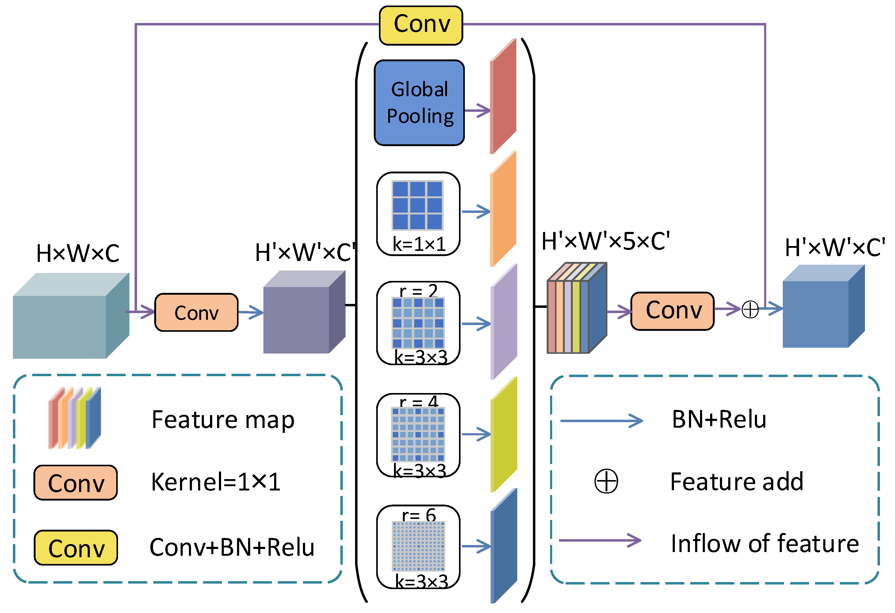
2.2. Multi-Scale Context Fusion Module

In the proposed framework, SMCF combines the advantages of DeepLabv3 [32] and Res-Net [33], as shown in Figure 3. DeepLabv3 and ResNet are two classic and representative architectures in deep learning. The structure of the DeepLab series uses different expansion rates to expand the receptive field of the model. Compared with the traditional convolution operation, the atrous convolution does not increase the number of parameters and maintains the same feature resolution. In addition, we introduce atrous convolution to improve the network’s ability to extract image features. Usually, pooling layers or convolutional layers with stride are used in the network structure for downsampling to expand the receptive field of the model. However, too many downsampling operations can cause the loss of feature information, which is not conducive to model learning and can increase the complexity of upsampling. To alleviate the above problem, let the network model keep the model receptive field constant or large while reducing the downsampling operation. We use artrous convolution [34] instead of standard convolution to increase the perceptual field of the convolution kernel in MSMB-Net. ResNet uses a residual connection mechanism to avoid the bursting and elimination of gradients, which also accelerates network convergence. Mathematically, the calculation formula of the atrous convolution under the two-dimensional signal is (1)
y [ i ] = k = 1 n [ x [ i ] + r k ] × w [ k ]
where x [ i ] is the input signal, w [ k ] is the kth parameter of the filter, k is the size of the filter, y [ i ] is the output signal, and r is the expansion rate. For a convolution filter with a size of k × k , the size of the obtained expansion filter is k r × k r , where k r = k + ( k 1 ) × ( r 1 ) . Therefore, those with a large expansion rate have a large receptive field.
Due to the complex structure of fundus retinal images, large variation in segmentation target size and low background contrast, the SMCF module is proposed in this paper for the better segmentation of retinal images with different sizes and to alleviate the problem of blurred optic disc optic cup boundary segmentation. In this paper, the SMCF module captures multi-scale features using skip connections and atrous convolution with different expansion rates. This is used to achieve the precise segmentation of blood vessel edges, tiny blood vessels, and optic disc cup boundaries. First, use 1 × 1 convolution to halve the number of feature mapping channels of the SMCF module, which can increase the speed of the model. Then, use the global average pooling layer and four parallel convolutional layers to capture feature information. The global average pooling layer uses bilinear interpolation to obtain image-level global context information [35]. Finally, the features captured by parallel convolution are merged into the model. Among them, the calculation of the kth pixel among image-level features is shown in Formulas (2) and (3)
r k = w = 0 W h = 0 H R k ( w , h ) W × H , w W , h H
g a p k = G B I ( r k )
where, in r k = [ r 1 , r 2 , , r k ] , k is an input characteristic diagram of the channel number, w is an input characteristic diagram of the width, h is the input feature high, g a p k = [ g a p 1 , g a p 2 , , g a p k ] , and G B I ( · ) is bilinearly upsample.

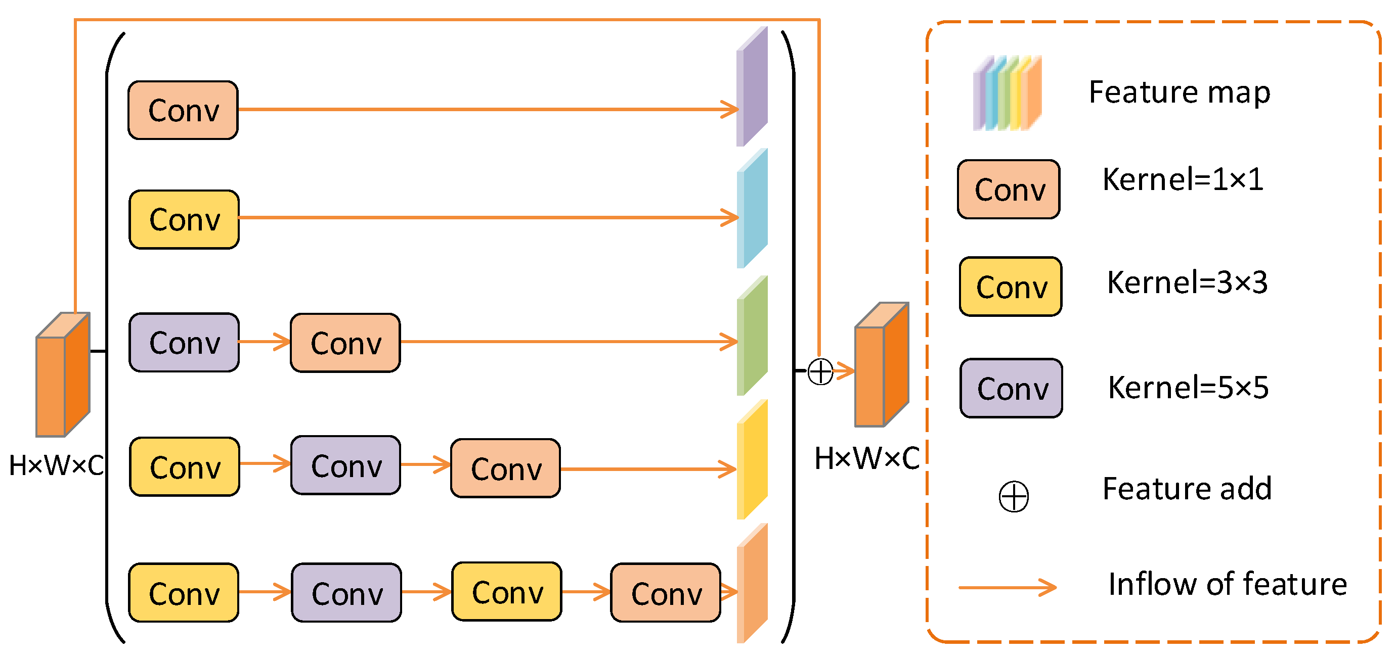
2.3. Multi-Branch Convolution Module

In medical images, the varying size of segmented objects has always been a problem in segmentation tasks. For example, retinal blood vessels vary in thickness. In this article, MBCM is proposed to alleviate this problem.
As shown in Figure 4, this mainly relies on combining multiple effective convolution kernels to detect targets of different sizes. Usually, the convolution of the large receptive field extracts the large target feature. The convolution of the small receptive field is more suitable for the recovery of small targets. The MBCM module has five cascaded branches. In each branch, convolution operations with different kernel sizes will obtain feature information maps of different sizes. In the last three branches, 1 × 1 convolution is used to correct linear activation, which reduces the dimensionality and computational cost of weights. Finally, after feature transfer, the feature maps of the five branches are added to the original feature maps. This obtains a feature map of the same size as the original feature map.

2.4. Side-Output Rebuilding Layer

In the decoder part, the feature maps of different channel numbers are aggregated. In this way, a sufficiently high-resolution image is obtained to restore the features. This improves the utilization of each layer of channels. Figure 5 details the design of the Side-output Rebuilding Layer (SRL). In the figure, the symbol C indicates the number of channels. In this paper, an SRL is proposed to obtain spatial information while aggravating the deep and shallow semantic information. In the upsampling process, SRL layers are used instead of the deconvolution or bilinear interpolation methods to reduce the number of parameters while keeping the some learning capability for the network. Assuming that the dimension of our input feature map is W × H × ( d × d × C ) , where d is the upsampling factor, we can obtain the feature map with dimension ( W × d ) × ( H × d ) × C by SRL algorithm. The advantages of SRL as an upsampling method are as follows: (1) Compared with the deconvolution method, SRL does not add extra parameters and computational overhead, which can improve the speed of MSMB-Net. Additionally, SRL is learnable, so it can capture and recover the lost details in downsampling; (2) Compared with the bilinear interpolation method, the bilinear interpolation for upsampling method is not able to learn, although it does not need to bring in extra parameters and computational overhead. This makes it impossible to accurately restore the lost feature information. Therefore, SRL combines the advantages of both methods.
First, SRL periodically rearranges the information in the four-layer feature maps (L1, L2, L3, L4) of the decoded path. The height and width of the feature map are expanded by upsampling factors (1, 2, 4, 8) to achieve the effect of reducing the number of channels and increasing the size of the feature map. The implementation process is shown in Algorithm 1. After the scale reconstruction of the feature map by SRL, the segmentation results and edge information of the reconstructed feature map are refined using 3 × 3 and 1 × 1 convolution operations. The SRL layer mainly performs eight and 16 specific channel convolutions on the four-layer output feature R of the MSMB-Net decoding path, which generates the corresponding SRL_32 branch and SRL_64 branch. After the feature map passes through the SRL, the SRL_32 branch and the SRL_64 branch apply two 3 × 3 convolutions and a 1 × 1 convolution to refine the feature information of its edges, which means that MSMB-Net achieve better segmentation accuracy.
Algorithm 1: Side-output Rebuilding Layer
Input:
Feature map: x R N × h × w × c .             Batch of feature maps: N.
Height of the feature map:h.            Width of the feature map:w.
Channel c of the feature map:c.        Downsampling factor:d.
Output:
Feature map after scale rebuilding: x R N × ( w × d ) × ( w × d ) × c d × d
1:
c o u t = c d × d
2:
fori in c do
3:
for j in h do
4:
  for k in w do
5:
    c = i mod c o u t
6:
    h = j × d + c o u t d
7:
    w = k × d + c o u t mod d
8:
    x [ : , h , w , c ] = x [ : , j , k , i ]
9:
  end for
10:
end for
11:
end for

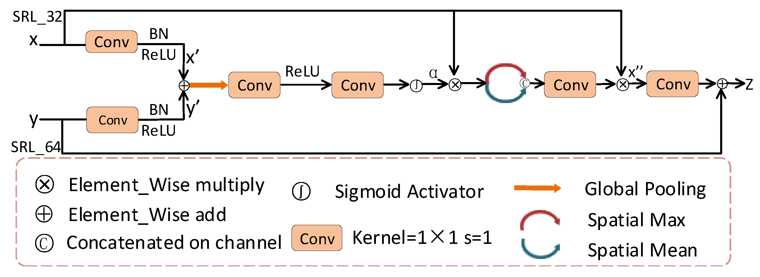
2.5. Attention Module

The attention module was inspired by CBAM [36]. To obtain good segmentation performance, we embed the proposed attention module into the MSMB-Net. The attention module can highlight the important regions of fundus images and optic disc visual cups, filter out the background noise, and solve the information loss problem caused by SRL reconstruction features. For a given input image, channel attention aims to establish the correlation between channels. It enhances the specific semantic response ability of the channel and emphasizes the meaningful parts. As a supplement to channel attention, spatial attention aims to enhance the expression of their respective features through the association of any two pixels. In this way, the features in the spatial position generate attention. The attention mechanism is sensitive to features, which allows the network to obtain detailed information that needs attention. It effectively selects the features generated by the SRL module, which suppresses information that is useless for segmentation. This is very important for decoders without any supervision information.
The attention module proposed in this paper is shown in Figure 6. First, the feature maps x and y of SRL_32 branch and SRL_64 branch are input to the attention module through the convolution layer. The corresponding feature vectors are obtained after global pooling. The gating coefficients α are obtained by sigmoid activation. We used spatial maximization and spatial averaging for the α × x feature maps. The feature maps obtained by spatial maximization and spatial averaging are concatenated. The feature maps obtained by concatenating have interdependent information with x. This allows the model to efficiently select more detailed information that needs attention. In this way, the spatial tolerance of the model is improved. Finally, x and y are summed to obtain the final output feature z, which is used for pixel classification and improves the sensitivity of the channel features. The experimental results demonstrate that the attention module enables the MSMB-Net model to achieve higher specificity and accuracy.

3. Dataset and Evaluation

3.1. Dataset

The method proposed in this paper was verified on four public datasets: DRIVE [37], STARE [38], CHASE [39] and Drishti-GS1 [40].
DRIVE dataset consists of 40 retinal fundus blood vessel images. The size of each image is 565 × 584 . The dataset comes from the Dutch diabetic retinopathy screening program. Among them, 33 did not show any signs of diabetic retinopathy and seven showed signs of mild early diabetic retinopathy. (http://www.isi.uu.nl/Research/Databases/DRIVE/ accessed on 24 February 2021);
STARE dataset consists of 20 retinal fundus images. The size of each image is 700 × 605 . Among them, there were 10 images of healthy subjects and 10 pathological images with overlapping blood vessels. (https://cecas.clemson.edu/~ahoover/stare/ accessed on 24 February 2021);
CHASE dataset consists of the left and right eyes of 14 students. The size of each image is 1280 × 960 . Compared with DRIVE and STARE, the image has uneven background illumination, poor contrast of blood vessels and narrow arteries. (https://blogs.kingston.ac.uk/retinal/chasedb1/ accessed on 24 February 2021);
Drishti-GS1 dataset consists of 101 retinal fundus images, including 31 normal images and 70 diseased images. Its images vary in size. Each image is manually marked by four ophthalmologists. The average optic disc and optic cup area are regarded as standard areas. (https://cvit.iiit.ac.in/projects/mip/drishti-gs/mip-dataset2/Home.php accessed on 24 February 2021).

3.2. Implementation Details

The method in this paper is based on the deep learning open source framework Pytorch [41], Linux operating system, Intel(R) Xeon(R) Gold 5218 2.30GHz CPU and Quardro RTX 6000 24G GPU. Its running memory is 187G. In the training phase, the Adam [42] optimizer was used for gradient descent. The Softmax function was used for final classification. The learning rate l r was initialized to 0.001, which attenuates the learning rate through the Plateau [43] method. To prevent the risk of overfitting and to improve the model performance, a random dynamic extraction of small batches of patches was taken to train the network. The patch size was 48 × 48 , the batch initialization was 32, and the training period was 200. The probability thresholds in the four standard datasets were set to 0.46, 0.5, 0.48 and 0.3, respectively. The total number of parameters of the model proposed in this paper is 58.361 MB. The loss function uses a cross-entropy loss function. This is defined as follows (4)
L ( p i , q i ) = 1 n i [ p i log q i + ( 1 p i ) log ( 1 q i ) ]
where p i represents the real label and q i represents the predicted image.
For DRIVE, we followed the criteria given by the data publisher and used 20 images for training and 20 images for testing. For CHASE, the method proposed in [44] was used, which uses 20 images for training, and eight images from four children were selected for testing. For STARE, the “leave-one-out” method proposed in the literature [45,46,47] is used, which uses 19 images for training and the remaining images for iterative testing. For the 101 retinal fundus images of the Drishti-GS1 dataset, 50 images were used and 51 images were used for testing. In the test phase, each test image of each dataset is extracted sequentially with image patches in a sliding window of the same size as the training phase.
The preprocessing method in [48] is used in the Drishti-GS1 dataset, which polarizes the original image to effectively refine the boundary portion of the optic disc view cup. Data augmentation was performed using the method of optic disc centroid image detection [49] to extract images of 10 different sizes for training. In the testing phase, only the test image size of 700 × 700 was extracted for testing, and the image was scaled to 512 × 512 for input into the network. Finally, the generated predicted images were filled to the same size as the original image.

3.3. Performance Evaluation

The influence of F1 score (F1), Accuracy (Acc), Sensitivity (Se), Specificity (Sp) and ROC curve area on the segmentation results are analyzed by the confusion matrix. Boundary distance localization error (BLE) [50] and F1 score are used to evaluate the performance of different segmentation methods. This is defined as follows (5)–(10):
A c c u r a c y = T P + T N T P + F P + T N + F N
S e s i t i v i t y = T P T P + F N
S p e c i f i c i t y = T N T N + F P
P r e c i s i o n = T P T P + F P
R e c a l l = T P T P + F N
F 1 s c o r e = 2 P r e c i s i o n × R e c a l l P r e c i s i o n + R e c a l l
where T P indicates the number of pixels that labeled the vascular pixels correctly, T N indicates the number of pixels that labeled the background correctly, F P is the number of pixels that failed to label the vascular pixels correctly, and F N is the number of pixels that failed to label the background pixels correctly.
Because the F1 score is not suitable for boundary segmentation evaluation, BLE is used to evaluate the segmentation results of the Drishti-GS1 dataset in this paper. It uses the average BLE to measure the boundary distance (in pixels) between the boundary segmentation (Co) of the optic disc region and the ground truth (Cg). BLE is defined as (11)
B L E ( C g , C o ) = 1 N n = 1 N d g θ d o θ
where d g θ represents the radial Euclidean distance from the predicted boundary point to the center of mass in the direction θ . d o θ represents the radial Euclidean distance from the ground truth boundary point to the center of mass in the direction θ . In the experimental evaluation, 24 equidistant points are set. The ideal value of BLE is θ .

4. Experimental Results and Discussion

4.1. Compare the Results of the Improved Model

To analyze the effect of the improvement, we compare the performance of the improved network and the Basic network model. Under the same parameter settings, the DRIVE, STARE, CHASE and Drishti-GS1 test datasets were used to verify the model. The effectiveness of the network is verified by combining SMCF, MBCM, SRL and the attention mechanism module proposed in this paper. In Table 1, SMCF represents the multi-scale context information fusion module, and MBCM represents the multi-branch convolution module, SRL represents the side-output rebuilding layer, Att represents the attention mechanism module, and MSMB-Net represents SMCF + MBCM + SRL + Att. All bolded data in the table indicate optimal results.
Table 1 shows the experimental results for the five models on the DRIVE dataset. In the table, “Basic” stands for U-Net with multiscale input, which is in the form of side input, as mentioned in the methodology. The results of the Basic experiments show that the Unet architecture is able to segment the retinal vessels effectively and achieve good results. By comparing the experimental results of the first row and the second row, it is found that the F1 score has improved in all three datasets. This shows that SMCF helps the encoder to partially extract multi-scale, high-level semantic features. The extracted local context information is conducive to obtaining high-resolution, high-level semantic feature maps. Comparing the second and third row shows that the SRL proposed in this paper improves the segmentation effect of retinal blood vessels by expanding the receptive field of the vascular characteristics in the decoder. The accuracy of STARE and CHASE datasets has improved. F1 scores have also improved in all three datasets. The fourth line shows that the proposed MBCM re-encodes the features extracted by SMCF, which is beneficial to the segmentation result. MBCM uses the convolution of different kernel sizes to change the combination of features to improve the fracture of small blood vessels in the segmented image. The proposed MBCM improves the F1 score and sensitivity of the experiment. Comparing the fifth row with other rows shows that the MSMB-Net network architecture can segment the retinal fundus blood vessels very well. The experimental data show that the MSMB-Net segmentation effect is the highest. The F1/Accuracy score reached 0.8320/0.9708, 0.8469/0.9753 and 0.8190/0.9767 on the DRIVE, STARE and CHASE datasets. Compared with the Basic network model, the sensitivity was increased by 3.84%, 2.9% and 1.51%, and the specificity was increased 0.11%, 0.51% and 0.09% respectively.The data format in the table is:mean/standard deviation.
Table 2 shows the experimental results for the five models on the Drishti-GS1 dataset. As with the experiments on the DRIVE, STARE, and CHASE datasets, we added the SMCF, MBCM, SRL, and attention modules to MSMB-Net in order to validate their effectiveness. The data format of BLE in the table is average/standard deviation. Optic stands for joint optic disc view cup segmentation. In order to further verify the effectiveness of the MSMB-Net network architecture, experiments were performed on the optic disc cup on the Drishti-GS1 dataset. When SMCF is used, the segmentation performance of the model significantly improves. According to the segmentation results of the optic disc and the optic cup, the F1 score is 0.84% and 1.25% higher than that of the Basic model, while the BLE decreases by 1.131px and 1.239px. With the addition of SRL, the model integrates low-level and high-level context information, which can effectively exclude avascular areas and more accurately segment the boundaries of the optic cup. In the optic disc and optic cup segmentation results, the F1 scores are improved by 1.37% and 1.65% compared with Basic. BLE decreased by 1.917px, 2.442px, especially the sensitivity to the optic cup, which reached 0.9599. The MBCM module further extracts global context information to obtain high-resolution advanced semantic feature maps, which significantly improves the segmentation results of the video disc. The F1 score is 1.46% higher than Basic, BLE is lowered by 2.868px, and the sensitivity is higher than Basic. 2.99%. It can be seen from the fifth row of the table that MSMB-Net has better results than other models. The F1 score is 1.78% and 3.5% higher than that of Basic, and BLE is significantly reduced by 3.338px and 6.511px. This shows that the combination of convolutional neural network and attention has a significant effect on the segmentation of the optic disc and cup. In the segmentation results of the combined optic disc cup, the F1 score is 1.74% higher than the Basic model. The sensitivity and specificity are also stronger, which can also explain the effectiveness of the MSMB model proposed in this paper for optic disc cup segmentation. The data format in the table is: mean/standard deviation.

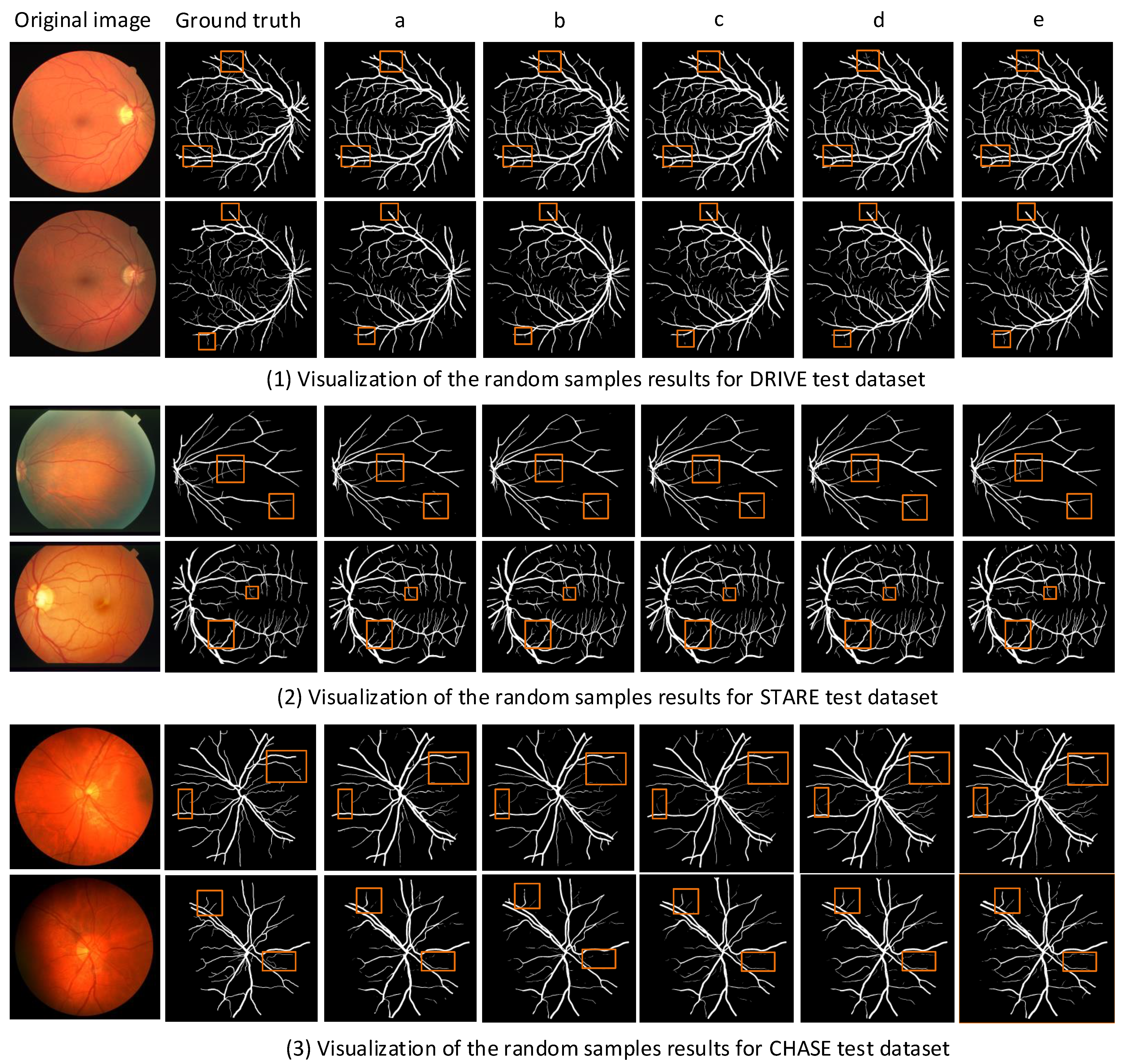
4.2. Retinal Vessel Segmentation

To demonstrate the effectiveness of our method in vessel segmentation, we evaluated our method on four datasets using the previously proposed unsupervised and supervised methods. Table 3, Table 4 and Table 5 show the segmentation results on the DRIVE, STARE and CHASE datasets compared to other methods. In this paper, we mainly use sensitivity, specificity, accuracy and F1 metric as evaluation metrics. As can be seen from the tables, the segmentation results of the supervised methods are generally better than those of the unsupervised methods, and the accuracy and F1 scores of the supervised methods are higher.
On the DRIVE dataset, MSMB-Net achieved good results in terms of specificity, accuracy and F1 scores. The experimental results are shown in Table 3. The methods of UNet and R2U-Net will segment blood vessels thicker than real blood vessels, so the accuracy of segmentation is also lower. When using the Ce-net method to segment pathological images, the segmentation results will produce a lot of noise. Furthermore, the lesion area is divided into blood vessels, so the sensitivity of the network is high and the accuracy is low. IterNet uses weight sharing and skip connections to reprocess the segmented images, which can find blurred vessel details. In this paper, skip connections and atrous convolution are used to fully fuse the features of the shallow layer and the deep layer, and restore the lost small blood vessels. The specificity of the network is improved and the result of segmentation is more accurate. In terms of F1 score and accuracy, the performance of MSMB-Net is 1.27% 0.22% higher than that of HAnet.
On the STARE dataset, pathology images segmented with Sine-Net had vascular segmentation errors. The visually segmented retinal vessels were thicker than the actual vessels, and thus had low sensitivity and high specificity. The experimental results are shown in Table 4. The visually segmented retinal vessels were thicker than the actual vessels, and thus had low sensitivity and high specificity. The MSMB-Net method segmented the background image and blood vessels more accurately, which is closer to the actual segmentation. The sensitivity of MSMB-Net is 87.6%, which is 3.91% higher than DUNet. However, the DUNet segmentation result is slightly higher than MSMB-Net in terms of F1 score and accuracy.
In the CHASE dataset, segmentation is difficult because of the uneven background brightness, poor contrast and wide arteries of the original image. The experimental results are shown in Table 5. Therefore, the model needs to have a stronger ability to extract feature information. MSMB-Net is superior to other methods in terms of sensitivity, specificity and accuracy, with an accuracy that is 1.89% higher than U-Net. R2U-Net up- and down-sampling loses the characteristics of small blood vessels, and the small receptive field settings cannot capture large-scale features. Therefore, the network sensitivity is weak. HAnet has the highest F1 score on this dataset, but it is not as accurate as MSMB-Net.
The local feature information of different ranges is effectively extracted by combining convolutional kernels of different sizes. The loss of feature information is mitigated using atrous convolution with different expansion rates. After fusing the feature information branches, the attention module obtains more useful feature information. This is beneficial to the final segmentation and effectively improves the segmentation accuracy of small blood vessels and blood vessel edge information. The comparative analysis of DRIVE, STARE and CHASE datasets shows that MSMB-Net has better performance and robustness.

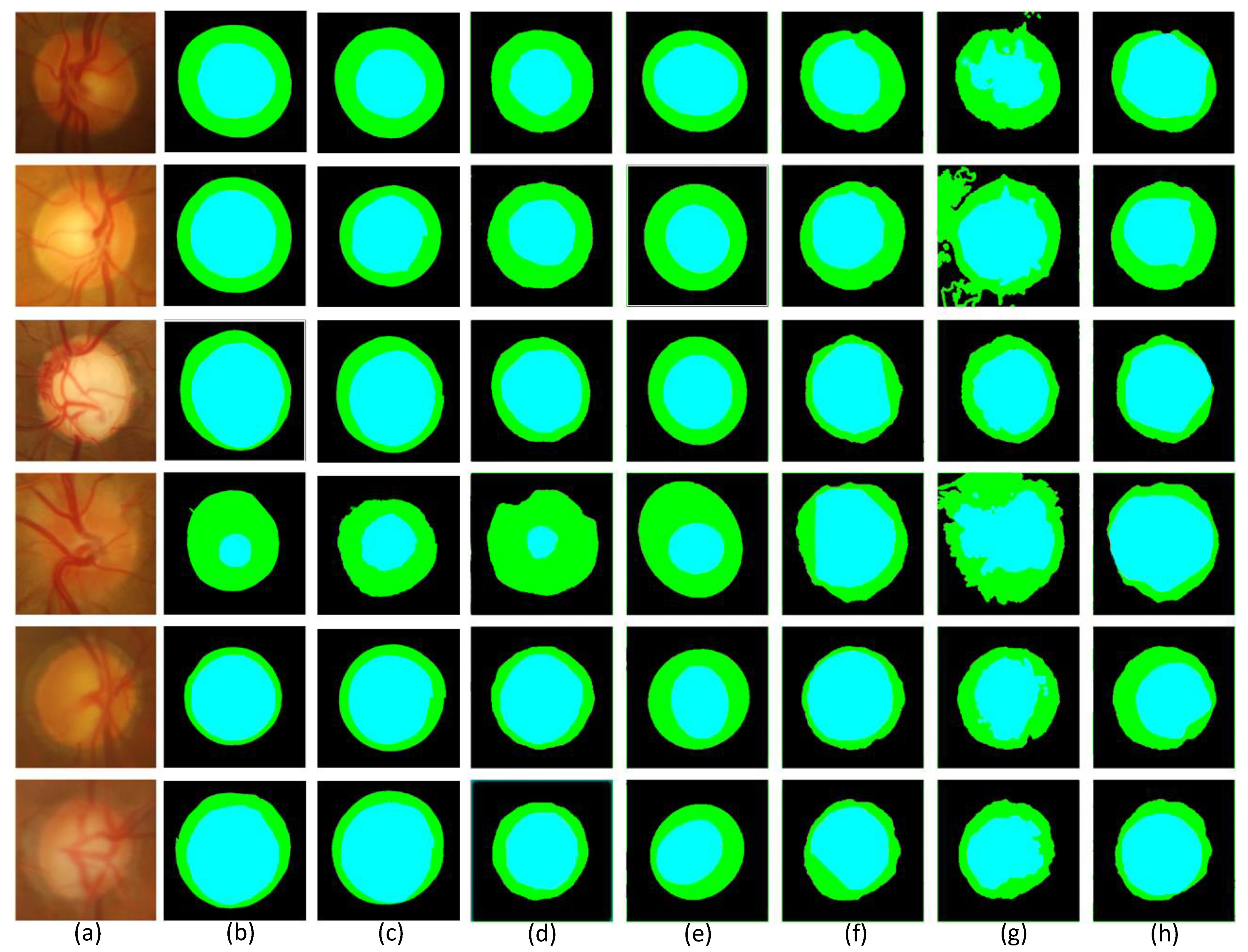
4.3. Optic Disc and Optic Cup Comparison of Different Methods

To illustrate the generalizability of MSMB-Net in the retinal image segmentation task, we compared our method with others using some existing methods on the Drishti-GS1 dataset. Table 6 and Table 7 show the segmentation performance on the Drishti-GS1 dataset compared to other methods. The sensitivity, specificity and accuracy are not given in the extensive literature in the tables. As can be seen from the table, our method performs well in terms of specificity and accuracy. The data format of Dice in the table is: mean/standard deviation.
MSMB-Net achieved the best performance in terms of specificity, accuracy and BLE evaluation indicators. In addition, the fundus optic disc segmentation also achieved the best performance on the Dice index. In the segmentation results of the fundus optic cup, MSMB-Net is 4.84% and 3.12px higher than UNet in Dice and BLE. Stack-u-net widens the network through two U-Nets, but the parameters of the model increase and the complexity of the model structure increases. RACE-net uses a recurrent neural network method to segment the optic disc and the optic cup. There are a large number of shared parameters in the network structure, which makes the network learning ability insufficient. Although Ce-net has achieved good results in the segmentation of the optic disc, it does not segment the optic cup well. CDED-Net eliminates the pre-processing and post-processing to reduce the calculation cost, and the Dice index of the fundus optic cup segmentation reached 92.4%. However, in optic disc segmentation, MSMB-Net is 0.11% and 1.85% higher in specificity and accuracy than CDED-Net. In contrast, the method in this paper is better than other methodsof optic disc and cup segmentation, which fully proves the generalization ability and effectiveness of MSMB-Net.

4.4. Different Segmentation Quantitative Analysis of the Results

In order to observe the difference of segmentation results more visually, we compare the segmentation visualization images of each model in the ablation experiment. The advantages of MSMB-Net can be seen from the visualized images. Figure 7 and Figure 8 show the visualization results of each model for DRIVE, STARE, CHASE and Drishti-GS1 datasets, respectively.
Figure 7 shows the comparison of the segmentation result images of each model on the DRIVE, STARE and CHASE datasets. In the figures, (1) shows the visualization results of random samples from the DRIVE test dataset, (2) shows the visualization results of random samples from STARE test dataset, and (3) shows the visualization results of random samples from the CHASE test dataset. The yellow boxes in the figure indicate that different network models have different effects on the local segmentation regions of the blood vessels. We can find some broken and mis-segmented vessel segments by zooming in on the yellow box. At the same time, it is observed that the combination of SMCF modules has a certain repair effect on the break of small blood vessels than the combination without these modules. In addition, from the segmentation results, the MSMB-Net model is more accurate for the segmentation of some small blood vessels.
Each row of Figure 8 shows the visualization segmentation results for the optic disc and optic cup corresponding to each model on the Drishti-GS1 dataset. Since the segmented images were too small to be easily observed, we zoomed in on the visualization results for the optic discs and optic cups.The first row of the figure shows the original image of the optic disc cup along with the corresponding ground truth and the corresponding magnified image. The second row is the segmentation visualization of the baseline network model experiment. The third row is the segmentation visualization of the network model, adding the SMCF module. The fourth row is the segmentation visualization of the network model joining the SRL layer. The fifth row is the segmentation visualization of the network model, adding the MBCM module. The sixth row is the segmentation visualization of MSMB-Net. In addition, we can determine the difference between the different network models by looking at the magnified edges in the optic disc view cup visualization. Comparing the partially enlarged images of different module combinations, we can see the effectiveness of MSMB-Net segmentation. The optic disc cup area is also enlarged and displayed. Through the enlarged image, it can be seen that the contour of the MSMB-Net model is more consistent with the real label during the segmentation of the optic disc. Compared with other combined models, the segmentation contour of the optic cup of the MSMB-Net model is more accurate and perfect than other models.
In the following experiments, MSMB-Net is compared with some existing methods (e.g., UNet, Ce-net). In this paper, the effectiveness of MSMB-Net is illustrated by comparing the visualization of MSMB-Net with the visualization of existing methods.
Figure 9 shows the segmentation visualization of two retinal images on the DRIVE dataset. The first line is an image of the retina of a diabetic patient. The second line is the retina image of a normal person. The red box in the figure indicates the local magnification part, and the difference with other models can be found with the magnified image. We observe that Unet and Ce-net have unclear and inaccurate segmentation of fine vessels. The visualization results show that MSMB-Net is effective for the segmentation of small blood vessels. The small blood vessels segmented by the UNet method are unclear and blurred. When the Ce-net method is used to segment retinal blood vessels, the segmentation of small blood vessels is slightly better than UNet. However, it is easy to mistakenly segment the diseased area into retinal blood vessels, resulting in a poor segmentation effect. In the method used in this paper, the SMCF module is used to expand the range of the receptive field and reduce the loss of characteristic information. Therefore, the characteristics of small blood vessels and lesion areas are better restored, which makes the segmentation result more accurate.
In the Drishti-GS1 dataset, this paper also provides an experimental comparison of MSMB-Net with other methods.
Figure 10 shows the results of the visualization comparison of MSMB-Net with other methods for the same image. The blue part of the figure represents the optic cup and the green part represents the optic disc. By comparing the blue part and the green part with the ground truth in the figure, we can find significant differences in the visualization of the optic disc and optic cup by different network models, especially in the segmentation of the edges of the optic disc and optic cup and the accuracy of the segmentation. The experimental results show that MSMB-Net is more accurate for the boundary segmentation of the optic disc cup. The result of BCRF segmentation of the optic disc is not ideal. The boundaries segmented by the Superpixel method are all regular ellipses, while the segmentation results of the optic disc cup using the Multiview, Graph Cut prior and Vessel bend methods are inaccurate and the boundaries are chaotic. For the method in this paper, the MBCM module is used to realize the feature extraction of objects of different sizes, which makes the boundary segmentation more accurate.

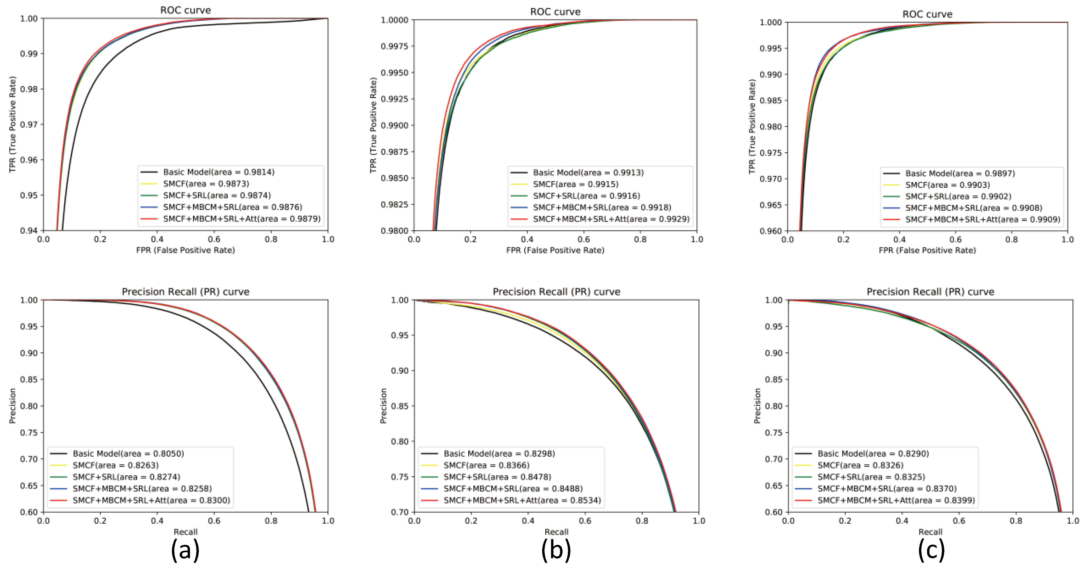
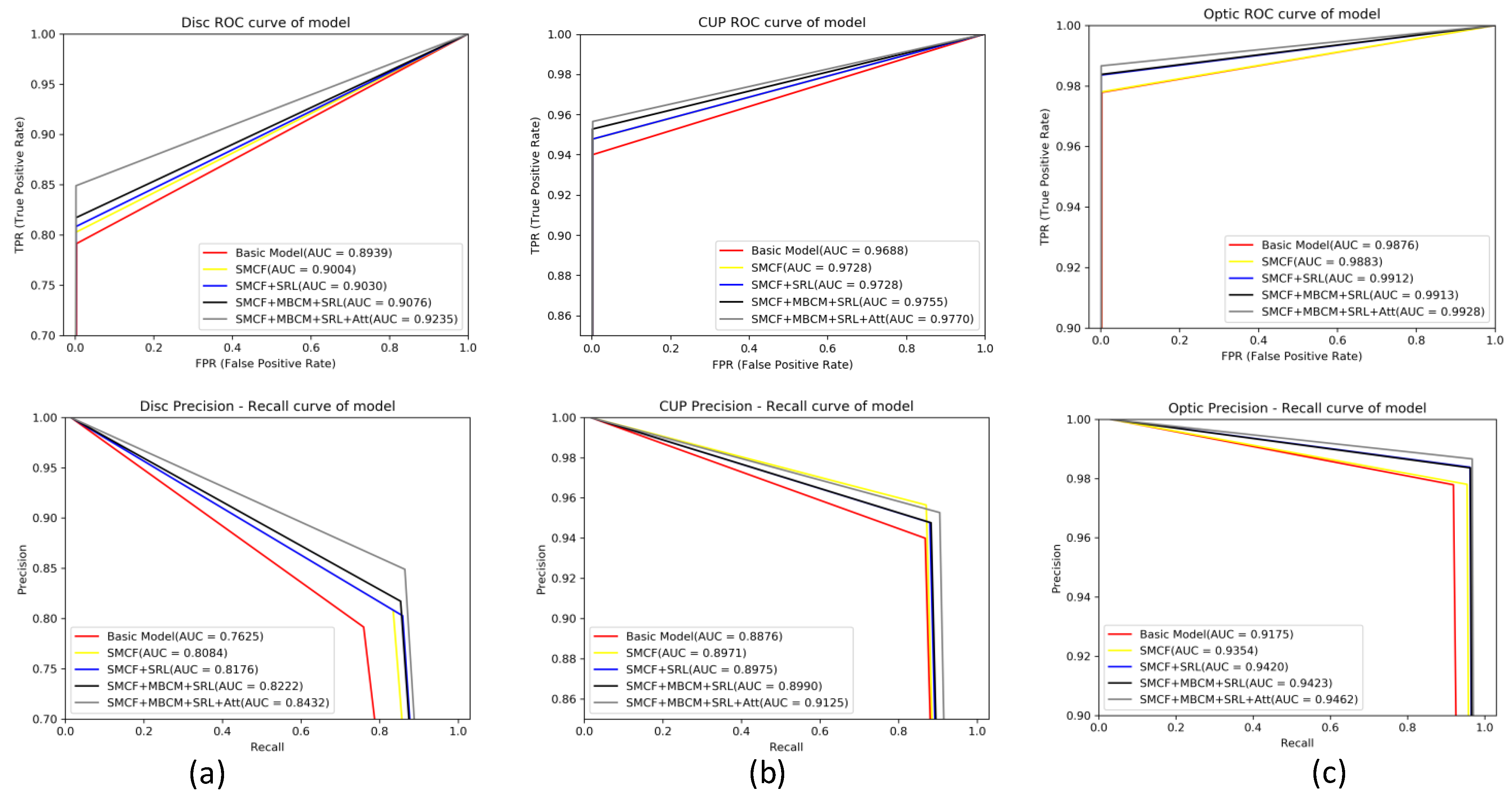
4.5. Evaluation of ROC Curve and PR Curve

In this set of experiments, we compared the receiver operating characteristic (ROC) curves and precision recall (PR) curves for each model on four datasets. On the Drishti-GS1 dataset, we also compared the BLE error statistics for each model.
In Figure 11, the first row is the ROC plot and the second row is the PR plot. The larger AUC value in the plot indicates the higher efficiency of the model, i.e., the larger area of the ROC and PR curves. In the figure, (a) indicates the ROC curve and PR curve plot for each model on the DRIVE dataset, (b) indicates the ROC curve and PR curve plot for each model on the STARE dataset, and (c) indicates the ROC curve and PR curve plot for each model on the CHASE dataset. Experimental results show that MSMB-Net has higher ROC and PR AUC values than other models. The ROC AUC values on the DRIVE, STARE and CHASE datasets are 0.9879, 0.9929 and 0.9909, and the PR AUC values are 0.8300, 0.8534 and 0.8399. Compared with the Basic model, the MSMB-Net model can extract deeper characterization features, which can better segment background information and offer finer blood vessel information. It can be found in the figure that the curves of MSMB-Net are all increasing at a positive rate, which shows that the performance of the proposed method is better than other combined model methods.
Figure 12 shows the comparison result of the BLE error statistical value box plot of each model in the Drishti-GS1 dataset. The first line is the BLE error statistical value box plot of the optic disc and the second line is the BLE error statistical value box plot of the optic cup. Figure depicts the error distribution of the BLE at 15-degree intervals over 360 degrees in horizontal coordinates, and the average error, median, and maximum and minimum errors and quadrature boxes for each test image (51 in total) in the same orientation (24 directions in total) are shown in vertical coordinates. The black horizontal lines represent the maximum and minimum error, the green horizontal lines represent the mean error, the orange squares represent the median, and the blue rectangles represent the quartile box. It can be seen from the figure that the MSMB-Net model has better results than other models. On the optic disc, the BLE error is reduced by 3.338 pixels compared with the Basic model. On the optic cup, the BLE error is 6.511 compared with the Basic model. The pixel variance is small. The influence of the optical cup is significantly improved, which also shows that the model in this paper is more accurate in segmentation of the optical cup.
Figure 13 shows the ROC curve and the PR curve of each model on the Drishti-GS1 dataset. In the figure, the first row is the ROC plot and the second row is the PR plot. Column (a) is the ROC curve and PR curve for each model on the Disc; column (b) is the ROC curve and PR curve for each model on the Cup; column (c) is the ROC curve and PR curve for each model on the Optic. It can be seen from the figure that the ROC and PR AUC values of MSMB-Net are higher than the other models. The AUC value of ROC of the optic disc is 0.9235, and the AUC value of PR is 0.8432. The AUC value of the ROC of the sight cup is 0.9770, and the AUC value of the PR is 0.9125. The AUC value of ROC of joint segmentation is 0.9928, and the AUC value of PR is 0.9462. The experimental results show that the MSMB-Net model can obtain the segmentation results of the optic disc more accurately and the segmentation performance of the boundary part of the optic cup is better. The combined segmentation results also show the effectiveness of the MSMB-Net model for the segmentation of the optic disc.

5. Conclusions

This paper proposes a segmentation network MSMB-Net for retinal images. In MSMB-Net, the SMCF module integrates parallel atrous convolutions with different expansion rates and skip connections, which capture more advanced context information and reduce parameters to improve the speed of the model. Segmentation has the problem of some features in the image becoming lost and difficult to recover. The MBCM module combines convolutions of different receptive field sizes to capture finer feature information. The SRL module fully integrates the shallow feature information and the deep feature information to recover the lost shallow information. It retains more spatial information. To improve the segmentation performance of the retinal image of the network model, the attention mechanism is embedded in MSMB-Net. Finally, we validated MSMB-Net on DRIVE, STARE and CHASE datasets. To demonstrate the generality of the network in this paper, we also performed experimental validation on the DRISHTI-GS1 dataset. The experimental results show that the proposed method in this paper performs better than some existing methods, such as UNet, Sine-Net and HAnet, for retinal vessel and optic disc optic cup segmentation.
However, the original image and the segmented image are processed again, which can improve the segmentation performance of the model. In future work, the paper will apply appropriate preprocessing and segmentation results in reprocessing methods to improve the performance of the network model. The model should also be applied to other medical images to demonstrate its versatility.

Author Contributions

Data curation, H.Y.; Methodology, W.L.; Resources, C.W.; software, W.L.; Supervision, Y.J.; Validation, W.L.; Writing—original draft, W.L.; Writing—review and editing, W.L. All authors have read and agreed to the published version of the manuscript.

Funding

This work was supported in part by the National Natural Science Foundation of China (61962054), in part by the the National Natural Science Foundation of China (61163036), in part by the 2016 Gansu Provincial Science and Technology Plan Funded by the Natural Science Foundation of China (1606RJZA047), in part by the 2012 Gansu Provincial University Fundamental Research Fund for Special Research Funds; Gansu Province Postgraduate Supervisor Program in Colleges and Universities (1201-16), in part by the Northwest Normal University’s Third Phase of Knowledge and Innovation Engineering Research Backbone Project (nwnu-kjcxgc-03-67).

Conflicts of Interest

The authors declare no conflict of interest. The funders had no role in the design of the study; in the collection, analyses, or interpretation of data; in the writing of the manuscript, or in the decision to publish the results.

References

  1. Khan, K.B.; Khaliq, A.A.; Jalil, A.; Iftikhar, M.A.; Ullah, N.; Aziz, M.W.; Ullah, K.; Shahid, M. A review of retinal blood vessels extraction techniques: challenges, taxonomy, and future trends. Pattern Anal. Appl. 2019, 22, 767–802. [Google Scholar] [CrossRef]
  2. Franklin, S.W.; Rajan, S.E. Computerized screening of diabetic retinopathy employing blood vessel segmentation in retinal images. Biocybern. Biomed. Eng. 2014, 34, 117–124. [Google Scholar] [CrossRef]
  3. Jonas, J.B.; Bergua, A.; Schmitz-Valckenberg, P.; Papastathopoulos, K.I.; Budde, W.M. Ranking of optic disc variables for detection of glaucomatous optic nerve damage. Investig. Ophthalmol. Vis. Sci. 2000, 41, 1764. [Google Scholar]
  4. Miao, Y.; Cheng, Y. Automatic extraction of retinal blood vessel based on matched filtering and local entropy thresholding. In Proceedings of the 8th International Conference on Biomedical Engineering and Informatics (BMEI), Shenyang, China, 14–16 October 2015; pp. 62–67. [Google Scholar]
  5. Kundu, A.; Chatterjee, R.K. Retinal vessel segmentation using Morphological Angular Scale-Space. In Proceedings of the 2012 Third International Conference on Emerging Applications of Information Technology, Kolkata, India, 30 November–1 December 2012; pp. 316–319. [Google Scholar] [CrossRef]
  6. Palomera-Perez, M.A.; Martinez-Perez, M.E.; Benitez-Perez, H. Parallel Multiscale Feature Extraction and Region Growing: Application in Retinal Blood Vessel Detection. IEEE Trans. Inf. Technol. Biomed. 2010, 14, 500–506. [Google Scholar] [CrossRef] [PubMed]
  7. Azzopardi, G.; Strisciuglio, N.; Vento, M.; Petkov, N. Trainable COSFIRE filters for vessel delineation with application to retinal images. Med. Image Anal. 2015, 19, 46–57. [Google Scholar] [CrossRef] [PubMed] [Green Version]
  8. Kumar, K.; Samal, D. Automated retinal vessel segmentation based on morphological preprocessing and 2D-Gabor wavelets. In Advanced Computing and Intelligent Engineering; Springer: Singapore, 2020; pp. 411–423. [Google Scholar]
  9. Tian, C.; Fang, T.; Fan, Y.; Wu, W. Multi-path convolutional neural network in fundus segmentation of blood vessels. Biocybern. Biomed. Eng. 2020, 40, 583–595. [Google Scholar] [CrossRef]
  10. Jainish, G.R.; Jiji, G.W.; Infant, P.A. A novel automatic retinal vessel extraction using maximum entropy based EM algorithm. Multimed. Tools Appl. 2020, 79, 22337–22353. [Google Scholar] [CrossRef]
  11. Marín, D.; Aquino, A.; Gegúndez-Arias, M.E.; Bravo, J.M. A new supervised method for blood vessel segmentation in retinal images by using gray-level and moment invariants-based features. IEEE Trans. Med. Imaging 2010, 30, 146–158. [Google Scholar] [CrossRef] [PubMed] [Green Version]
  12. Aslani, S.; Sarnel, H. A new supervised retinal vessel segmentation method based on robust hybrid features. Biomed. Signal Process. Control 2016, 30, 1–12. [Google Scholar] [CrossRef]
  13. Feng, Z.; Yang, J.; Yao, L. Patch-based fully convolutional neural network with skip connections for retinal blood vessel segmentation. In Proceedings of the IEEE International Conference on Image Processing (ICIP), Beijing, China, 17–20 September 2017; pp. 1742–1746. [Google Scholar]
  14. Mo, J.; Zhang, L. Multi-level deep supervised networks for retinal vessel segmentation. Int. J. Comput. Assist. Radiol. Surg. 2017, 12, 2181–2193. [Google Scholar] [CrossRef]
  15. Hu, K.; Zhang, Z.; Niu, X.; Zhang, Y.; Cao, C.; Xiao, F.; Gao, X. Retinal vessel segmentation of color fundus images using multiscale convolutional neural network with an improved cross-entropy loss function. Neurocomputing 2018, 39, 179–191. [Google Scholar] [CrossRef]
  16. Yan, Z.; Yang, X.; Cheng, K.T. A three-stage deep learning model for accurate retinal vessel segmentation. IEEE J. Biomed. Health Inform. 2018, 23, 1427–1436. [Google Scholar] [CrossRef]
  17. Ronneberger, O.; Fischer, P.; Brox, T. U-net: Convolutional networks for biomedical image segmentation. In International Conference on Medical Image Computing and Computer-Assisted Intervention; Springer: Cham, Switzerland, 2015; pp. 234–241. [Google Scholar]
  18. Alom, M.Z.; Hasan, M.; Yakopcic, C.; Taha, T.M.; Asari, V.K. Recurrent residual convolutional neural network based on u-net (r2u-net) for medical image segmentation. arXiv 2018, arXiv:1802.06955. [Google Scholar]
  19. Li, L.; Verma, M.; Nakashima, Y.; Nagahara, H.; Kawasaki, R. Iternet: Retinal image segmentation utilizing structural redundancy in vessel networks. In Proceedings of the IEEE Winter Conference on Applications of Computer Vision (WACV), Snowmass, CO, USA, 1–5 March 2020; pp. 3656–3665. [Google Scholar]
  20. Jin, Q.; Meng, Z.; Pham, T.D.; Chen, Q.; Wei, L.; Su, R. DUNet: A deformable network for retinal vessel segmentation. Knowl.-Based Syst. 2019, 178, 149–162. [Google Scholar] [CrossRef] [Green Version]
  21. Atli, İ.; Gedik, O.S. Sine-Net: A fully convolutional deep learning architecture for retinal blood vessel segmentation. Eng. Sci. Technol. Int. J. 2020, in press. [Google Scholar]
  22. Wang, D.; Haytham, A.; Pottenburgh, J.; Saeedi, O.; Tao, Y. Hard Attention Net for Automatic Retinal Vessel Segmentation. IEEE J. Biomed. Health Inform. 2020, 24, 3384–3396. [Google Scholar] [CrossRef]
  23. Zilly, J.G.; Buhmann, J.M.; Mahapatra, D. Boosting convolutional filters with entropy sampling for optic cup and disc image segmentation from fundus images. In International Workshop on Machine Learning in Medical Imaging; Springer: Cham, Switzerland, 2015; pp. 136–143. [Google Scholar]
  24. Sevastopolsky, A.; Drapak, S.; Kiselev, K.; Snyder, B.M.; Keenan, J.D.; Georgievskaya, A. Stack-u-net: Refinement network for image segmentation on the example of optic disc and cup. arXiv 2018, arXiv:1804.11294. [Google Scholar]
  25. Chakravarty, A.; Sivaswamy, J. RACE-net: A recurrent neural network for biomedical image segmentation. IEEE J. Biomed. Health Inform. 2018, 23, 1151–1162. [Google Scholar] [CrossRef] [PubMed]
  26. Shah, S.; Kasukurthi, N.; Pande, H. Dynamic Region Proposal Networks For Semantic Segmentation In Automated Glaucoma Screening. In Proceedings of the IEEE 16th International Symposium on Biomedical Imaging (ISBI 2019), Venice, Italy, 8–11 April 2019; pp. 578–582. [Google Scholar]
  27. Yu, S.; Xiao, D.; Frost, S.; Kanagasingam, Y. Robust optic disc and cup segmentation with deep learning for glaucoma detection. Comput. Med. Imaging Graph. 2019, 74, 61–71. [Google Scholar] [CrossRef] [PubMed]
  28. Ding, F.; Yang, G.; Liu, J.; Wu, J.; Ding, D.; Xv, J.; Cheng, G.; Li, X. Hierarchical Attention Networks for Medical Image Segmentation. arXiv 2019, arXiv:1911.08777. [Google Scholar]
  29. Gu, Z.; Cheng, J.; Fu, H.; Zhou, K.; Hao, H.; Zhao, Y.; Zhang, T.; Gao, S.; Liu, J. Ce-net: Context encoder network for 2d medical image segmentation. IEEE Trans. Med. Imaging 2019, 38, 2281–2292. [Google Scholar] [CrossRef] [PubMed] [Green Version]
  30. Kadambi, S.; Wang, Z.; Xing, E. WGAN domain adaptation for the joint optic disc-and-cup segmentation in fundus images. Int. J. Comput. Assist. Radiol. Surg. 2020. [Google Scholar] [CrossRef]
  31. Tabassum, M.; Khan, T.M.; Arslan, M.; Naqvi, S.S. CDED-Net: Joint Segmentation of Optic Disc and Optic Cup for Glaucoma Screening. IEEE Access 2020. [Google Scholar] [CrossRef]
  32. Chen, L.C.; Papandreou, G.; Schroff, F.; Adam, H. Rethinking atrous convolution for semantic image segmentation. arXiv 2017, arXiv:1706.05587. [Google Scholar]
  33. He, K.; Zhang, X.; Ren, S.; Sun, J. Deep residual learning for image recognition. In Proceedings of the IEEE Conference on Computer Vision and Pattern Recognition (CVPR), Las Vegas, NV, USA, 27–30 June 2016. [Google Scholar]
  34. Chen, L.-C.; Papandreou, G.; Kokkinos, I.; Murphy, K.; Yuille, A. Deeplab: Semantic image segmentation with deep convolutional nets, atrous convolution, and fully connected crfs. IEEE Trans. Pattern Anal. Mach. Intell. 2017, 40, 834–848. [Google Scholar] [CrossRef]
  35. Zhao, H.; Shi, J.; Qi, X.; Wang, X.; Jia, J. Pyramid scene parsing network. In Proceedings of the IEEE Conference on Computer Vision and Pattern Recognition (CVPR), Honolulu, HI, USA, 21–26 July 2017; pp. 2881–2890. [Google Scholar]
  36. Woo, S.; Park, J.; Lee, J.-Y.; Kweon, I.S. Cbam: Convolutional block attention module. In Proceedings of the European Conference on Computer Vision (ECCV); Springer: Cham, Switzerland, 2018. [Google Scholar] [CrossRef] [Green Version]
  37. Staal, J.; Abràmoff, M.D.; Niemeijer, M.; Viergever, M.A.; van Ginneken, B. Ridge-based vessel segmentation in color images of the retina. IEEE Trans. Med. Imaging 2004, 23, 501–509. [Google Scholar] [CrossRef] [PubMed]
  38. Hoover, A.D.; Kouznetsova, V.; Goldbaum, M. Locating blood vessels in retinal images by piecewise threshold probing of a matched filter response. IEEE Trans. Med Imaging 2000, 19, 203–210. [Google Scholar] [CrossRef] [Green Version]
  39. Owen, C.G.; Rudnicka, A.R.; Mullen, R.; Barman, S.A.; Monekosso, D.; Whincup, P.H.; Ng, J.; Paterson, C. Measuring retinal vessel tortuosity in 10-year-old children: Validation of the computer-assisted image analysis of the retina (CAIAR) program. Investig. Ophthalmol. Vis. Sci. 2009, 50, 2004–2010. [Google Scholar] [CrossRef] [Green Version]
  40. Chakravarty, A.; Sivaswamy, J. Glaucoma classification with a fusion of segmentation and image-based features. In Proceedings of the IEEE 13th International Symposium on Biomedical Imaging (ISBI), Prague, Czech Republic, 13–16 April 2016; pp. 689–692. [Google Scholar]
  41. Paszke, A.; Gross, S.; Chintala, S.; Chanan, G.; Yang, E.; De Vito, Z.; Lin, Z.; Desmaison, A.; Antiga, L.; Lerer, A.; et al. Automatic Differentiation in Pytorch. In Proceedings of the 31st Conference on Neural Information Processing Systems (NIPS 2017), Long Beach, CA, USA, 4–9 December 2017. [Google Scholar]
  42. Kingma, D.P.; Ba, J. Adam: A method for stochastic optimization. arXiv 2014, arXiv:1412.6980. [Google Scholar]
  43. Loshchilov, I.; Hutter, F. Decoupled weight decay regularization. arXiv 2017, arXiv:1711.05101. [Google Scholar]
  44. Zhuang, J. Laddernet: Multi-path networks based on u-net for medical image segmentation. arXiv 2018, arXiv:1810.07810. [Google Scholar]
  45. Soares, J.V.B.; Leandro, J.J.G.; Cesar, R.M.; Jelinek, H.F.; Cree, M.J. Retinal vessel segmentation using the 2-D Gabor wavelet and supervised classification. IEEE Trans. Med. Imaging 2006, 25, 1214–1222. [Google Scholar] [CrossRef] [Green Version]
  46. Jiang, Y.; Zhang, H.; Tan, N.; Chen, L. Automatic retinal blood vessel segmentation based on fully convolutional neural networks. Symmetry 2019, 11, 1112. [Google Scholar] [CrossRef] [Green Version]
  47. Dharmawan, D.A.; Li, D.; Ng, B.P.; Rahardja, S. A new hybrid algorithm for retinal vessels segmentation on fundus images. IEEE Access 2019, 7, 41885–41896. [Google Scholar] [CrossRef]
  48. Fu, H.; Cheng, J.; Xu, Y.; Wong, D.W.K.; Liu, J.; Cao, X. Joint optic disc and cup segmentation based on multi-label deep network and polar transformation. IEEE Trans. Med. Imaging 2018, 37, 1597–1605. [Google Scholar] [CrossRef] [PubMed] [Green Version]
  49. Wang, L.; Yang, S.; Yang, S.; Zhao, C.; Tian, G.; Gao, Y.; Chen, Y.; Lu, Y. Automatic thyroid nodule recognition and diagnosis in ultrasound imaging with the YOLOv2 neural network. World J. Surg. Oncol. 2019, 17, 12. [Google Scholar] [CrossRef] [PubMed] [Green Version]
  50. Chakravarty, A.; Sivaswamy, J. Joint optic disc and cup boundary extraction from monocular fundus images. Comput. Methods Programs Biomed. 2017, 147, 51–61. [Google Scholar] [CrossRef]
  51. Joshi, G.D.; Sivaswamy, J.; Krishnadas, S.R. Optic disk and cup segmentation from monocular color retinal images for glaucoma assessment. IEEE Trans. Med. Imaging 2011, 30, 1192–1205. [Google Scholar] [CrossRef]
  52. Joshi, G.D.; Sivaswamy, J.; Krishnadas, S.R. Depth discontinuity-based cup segmentation from multiview color retinal images. IEEE Trans. Biomed. Eng. 2012, 59, 1523–1531. [Google Scholar] [CrossRef]
  53. Cheng, J.; Liu, J.; Xu, Y.; Yin, F.; Wong, D.W.K.; Tan, N.-M.; Tao, D.; Cheng, C.-Y.; Aung, T.; Wong, T.Y. Superpixel classification based optic disc and optic cup segmentation for glaucoma screening. IEEE Trans. Med. Imaging 2013, 32, 1019–1032. [Google Scholar] [CrossRef]
  54. Zheng, Y.; Stambolian, D.; O’Brien, J.; Gee, C.J. Optic disc and cup segmentation from color fundus photograph using graph cut with priors. In International Conference on Medical Image Computing and Computer-Assisted Intervention; Springer: Berlin/Heidelberg, Germany, 2013; pp. 75–82. [Google Scholar]
Figure 1. (a) Healthy retina image (b) Diabetic retinopathy image with a lot of hemorrhage and exudate (c) Glaucoma image; the neuroretinal border zone between optic disc and optic cup is relatively narrow (d) Normal retina image; the ratio of VCD to VDD is small.
Symmetry 13 00365 g001
Figure 2. Multi-scale and multi-branch network (MSMB-Net) network structure.
Symmetry 13 00365 g002
Figure 3. SMCF module structure diagram.
Symmetry 13 00365 g003
Figure 4. MBCM module structure diagram.
Symmetry 13 00365 g004
Figure 5. Side-output Rebuilding Layer structure diagram.
Symmetry 13 00365 g005
Figure 6. Attention structure diagram.
Symmetry 13 00365 g006
Figure 7. Different models at different segmentation results of visualization of the dataset: (a) column is Basic, (b) column is SMCF, (c) column is SMCF + SRL, (d) column is SMCF + MBCM + SRL, (e) column is MSMB-Net.
Symmetry 13 00365 g007
Figure 8. Comparison of segmentation images of each model in the Drishti-GS1 dataset. (a) Original image (b) Segmentation image of disc (c) Partial segmentation image of disc (d) Segmentation image of cup (e) Partial segmentation image of cup (f) Segmentation image of optic (g) Partial segmentation image of optic.
Symmetry 13 00365 g008
Figure 9. Comparison of different segmentation results in the DRIVE dataset. (a) Image (b) Ground truth (c) MSMB-Net (d) UNet (e) Ce-net.
Symmetry 13 00365 g009
Figure 10. Compares the segmentation results in the Drishti-GS1 dataset. (a) Original retinal image (b) ground truth (c) MSMB-Net (d) BCRF [50] (e) Superpixel [53] (f) Multiview [52] (g) Graph Cut prior [54] (h) Vessel bend [51].
Symmetry 13 00365 g010
Figure 11. ROC plots and PR plots for each model on the DRIVE, STARE and CHASE datasets. (a) ROC curve and PR curve diagram of each model in the DRIVE dataset (b)ROC curve and PR curve diagram of each model in the STARE dataset (c) ROC curve and PR curve diagram of each model in the CHASE dataset.
Symmetry 13 00365 g011
Figure 12. Box plot of BLE statistical values of each model in the Drishti-GS1 dataset. (a) Basic, (b) SMCF model, (c) SMCF+SRL, (d) SMCF+MBCM+SRL, (e) MSMB-Net.
Symmetry 13 00365 g012
Figure 13. ROC curve and PR curve diagram of each model on the Drishti-GS1 dataset. Column (a) is the ROC curve and PR curve for each model on the Disc, column (b) is the ROC curve and PR curve for each model on the Cup, column (c) is the ROC curve and PR curve for each model on Optic.
Symmetry 13 00365 g013
Table 1. Comparison of model changes in DRIVE, STARE and CHASE datasets.
MethodsDRIVESTARECHASE
F1AccSeSpF1AccSeSpF1AccSeSp
Basic0.8263/0.01890.9707/0.00390.7957/0.05190.9864/0.00320.8307/0.02110.9742/0.00440.8470/0.05270.9848/0.00450.8081/ 0.01810.9754/0.00380.8220/0.03310.9857/0.0025
SMCF0.8280/0.01820.9705/ 0.00320.8093/0.05180.9860/0.00340.8317/0.01790.9743/0.00400.8476/0.04520.9848/0.00340.8140/ 0.01900.9762/0.00360.8256/0.03910.9863/0.0022
SMCF+SRL0.8292/0.01560.9702/0.00260.8240/0.04770.9843/0.00390.8336/0.01350.9747/0.00350.8512/0.03110.9849/0.00290.8150/0.01360.9763/ 0.00310.8273/0.03440.9863/0.0023
SMCF+MBCM+SRL0.8301/0.01430.9704/0.00280.8246/0.04870.9844/0.00380.8341/0.01190.9747/0.00320.8534/0.02990.9847/0.00320.8161/0.01680.9757/0.0045 0 . 8465 / 0 . 0290 0.9844/0.0020
MSMB-Net (ours) 0 . 8320 / 0 . 0136 0 . 9708 / 0 . 0026 0 . 8341 / 0 . 0471 0 . 9875 / 0 . 0032 0 . 8469 / 0 . 0110 0 . 9753 / 0 . 0034 0 . 8760 / 0 . 0211 0 . 9899 / 0 . 0020 0 . 8192 / 0 . 0165 0 . 9767 / 0 . 0034 0.8371/0.0280 0 . 9866 / 0 . 0020
Table 2. Comparison of model changes on the Drishti-GS1 dataset.
MethodsDiscCupOptic
F1AccSeBLEF1AccSeBLEF1AccSeSp
Basic0.9604/0.1010.9935/0.0030.8056/0.1257.327/6.1910.8834/0.1120.9935/0.0010.9417/0.08417.528/11.9640.9596/0.0310.9968/0.0020.9766/0.0310.9974/0.002
SMCF0.8280/0.0720.9949/0.0020.8180/0.1106.196/5.3880.8959/0.0960.9970/0.0010.9498/0.06316.289/10.5750.9687/0.0170.9979/0.0010.9775/0.0270.9985/0.001
SMCF+SRL0.9741/0.0690.9952/0.0020.8114/0.1105.410/4.8710.8999/0.1090.9968/0.001 0 . 9599 / 0 . 056 15.086/11.2860.9736/0.0150.9983/0.00090.9831/0.0210.9987/0.001
SMCF+MBCM+SRL0.9750/0.0550.9953/0.0020.8355/0.0814.459/2.2030.8995/0.1060.9969/0.0010.9558/0.06313.354/10.1110.9735/0.0110.9983/0.00070.9833/0.0160.9988/0.0009
MSMB-Net (ours) 0 . 9782 / 0 . 034 0 . 9959 / 0 . 001 0 . 8610 / 0 . 045 3 . 989 / 1 . 824 0 . 9184 / 0 . 091 0 . 9975 / 0 . 002 0.9560/0.050 11 . 017 / 9 . 240 0 . 9770 / 0 . 011 0 . 9985 / 0 . 0007 0 . 9862 / 0 . 018 0 . 9992 / 0 . 001
Table 3. Comparison of proposed methods with other methods in the DRIVE dataset.
TypeMethodsYearSeSpAccF1
Unsupervised methods2nd human expert 0.77430.98190.96370.7889
Miao et al. [4]20150.74810.97480.9597-
Kumar et al. [8]20190.75030.97170.9432-
Tian et al. [9]20190.86390.96900.9580-
Jainish et al. [10]2020--0.9657-
Supervised methodsMarín et al. [11]20100.76070.98010.9452-
Aslani et al. [12]20160.75450.98010.9513-
Feng et al. [13]20170.78110.98390.9560-
U-Net [17]20180.75370.98200.95310.8142
R2U-Net [18]20180.77920.98130.95560.8171
IterNet [19]20190.77350.98380.95730.8205
Ce-net [29]20190.8309-0.9545-
Sine-Net [21]20200.82600.98240.9685-
HAnet [22]20200.79910.98130.95810.8293
MSMB-Net (ours)20200.82830.98640.97080.8315
Table 4. Comparison of proposed methods with other methods in the STARE dataset.
TypeMethodsYearSeSpAccF1
Unsupervised methods2nd human expert 0.90170.95640.95220.7417
Miao et al. [4]20150.72980.98310.9532-
Azzopardi et al. [7]20150.77160.97010.9497-
Jainish et al. [10]2020--0.9703-
Supervised methodsMarín et al. [11]20100.69440.98190.9526-
Aslani et al. [12]20160.75560.98370.9605-
Mo et al. [14]20170.81470.98440.9674-
Hu et al. [15]20180.75430.98140.9632-
U-Net [17]20180.82700.98420.96900.8373
IterNet [19]20190.77150.98860.97010.8146
DUNet [20]20190.83690.98880.97730.8485
Sine-Net [21]20200.67760.99460.9711-
HAnet [22]20200.81860.98440.96730.8379
MSMB-Net (ours)20200.87600.98990.97530.8469
Table 5. Comparison of proposed methods with other methods in the CHASE dataset.
TypeMethodsYearSeSpAccF1
Unsupervised methods2nd human expert 0.67760.99460.9711-
Azzopardi et al. [7]20150.75850.95870.9387-
Tian et al. [9]20190.87780.96800.9601-
Supervised methodsMo et al. [14]20170.76610.98160.9599-
Yan et al. [16]20180.76410.98060.9607-
U-Net [17]20180.82880.97010.95780.7783
R2U-Net [18]20180.77560.98200.96340.7928
IterNet [19]20190.79700.98230.96550.8073
DUNet [20]20190.81550.97520.96100.7883
Sine-Net [21]20200.78560.98450.9676-
MSMB-Net (ours)20200.83310.98640.97670.8190
Table 6. Comparison of Disc results of different baseline methods on the Drishti-GS1 dataset.
MethodsYearSeSpAccDiceBLE
Vessel Bend [51]2011---0.9600/0.028.93/2.96
Multiview [52]2012---0.9600/0.028.93/2.96
Superpixel [53]2013---0.9500/0.029.38/5.75
Graph Cut [54]2013---0.9400/0.0614.74/15.66
U-Net [17]20150.96000.98000.97000.9500-
Zilly et al. [23]2015---0.9470-
BCRF [50]2017---0.9700/0.026.61/3.55
Stack-u-net [24]2018---0.9700/0.026.47/3.51
RACE-net [25]2018---0.9700/0.026.06/3.84
Shah et al. [26]2019---0.9600-
Yu et al. [27]2019---0.9738-
Ding et al. [28]2019---0.9721-
Ce-net [29]20190.97590.9990-0.9642-
WGAN [30]2020---0.9540-
CDED-Net [31]20200.97540.9973-0.9597-
MSMB-Net (ours)20200.96100.99840.99590.97823.98/1.82
Table 7. Comparison of Cup results of different baseline methods on the Drishti-GS1 dataset.
MethodsYearSeSpAccDiceBLE
Vessel Bend [51]2011---0.7700/0.2030.51/24.80
Multiview [52]2012---0.7900/0.1825.28/18.00
Superpixel [53]2013---0.8000/0.1422.04/12.57
Graph Cut [54]2013---0.7700/0.1626.70/16.67
U-Net [17]20150.96000.98000.97000.8500/0.1019.53/13.98
Zilly et al. [23]2015---0.8300-
BCRF [50]2017---0.8300/0.1518.61/13.02
Stack-u-net [24]2018---0.8900/0.0914.39/7.18
RACE-net [25]2018---0.8700/0.0916.13/7.63
Shah et al. [26]2019---0.8900-
Yu et al. [27]2019---0.8877-
Ding et al. [28]2019---0.8513-
Ce-net [29]20190.88190.9909-0.8818-
WGAN [30]2020---0.8400-
CDED-Net [31]20200.95670.9981-0.9240-
MSMB-Net (ours)20200.95600.99830.99750.918413.01/9.24
Publisher’s Note: MDPI stays neutral with regard to jurisdictional claims in published maps and institutional affiliations.

