Internal Learning for Image Super-Resolution by Adaptive Feature Transform

Abstract

Recent years have witnessed the great success of image super-resolution based on deep learning. However, it is hard to adapt a well-trained deep model for a specific image for further improvement. Since the internal repetition of patterns is widely observed in visual entities, internal self-similarity is expected to help improve image super-resolution. In this paper, we focus on exploiting a complementary relation between external and internal example-based super-resolution methods. Specifically, we first develop a basic network learning external prior from large scale training data and then learn the internal prior from the given low-resolution image for task adaptation. By simply embedding a few additional layers into a pre-trained deep neural network, the image-adaptive super-resolution method exploits the internal prior for a specific image, and the external prior from a well-trained super-resolution model. We achieve 0.18 dB PSNR improvements over the basic network’s results on standard datasets. Extensive experiments under image super-resolution tasks demonstrate that the proposed method is flexible and can be integrated with lightweight networks. The proposed method boosts the performance for images with repetitive structures, and it improves the accuracy of the reconstructed image of the lightweight model.

1. Introduction

For surveillance video systems, 4K high-definition TV, object recognition, and medical image analysis, image super-resolution is a crucial step to improve image quality. Single image super-resolution (SISR) algorithms, aiming to recover a high-resolution (HR) image from a low-resolution (LR) image, is challenging since that one LR image corresponds to many HR versions. SISR methods enforce some predetermined constraints on the reconstructed image to address the severe ill-posed issues, which include data consistency [1,2], self-similarity [3,4], and structural recurrence [5,6]. Example-driven SISR methods further explore useful image priors from a collection of exemplar LR-HR pairs and learn the nonlinear mapping functions to reconstruct the HR image [7,8,9,10].

The recently blooming deep convolutional neural network (CNN) based SR methods aim to exploit image priors from a large training dataset, expecting that enough training examples will provide a variety of LR-HR pairs. Benefiting from high-performance GPUs and large amounts of memory, deep neural networks have significantly improved SISR [11,12,13,14,15,16,17,18].

Although CNN-based SR methods achieve impressive results on data related to the prior training, they tend to produce distracting artifacts, such as over-smoothing or ringing results, once the input image cannot be well represented by training examples [6,19]. For example, when providing an LR image that is downsampled by a factor of two to a model trained for a downsampling factor of four or giving an LR image with building textures to a model trained on natural outdoor images, the well-trained model most probably introduces artifacts.

To address this issue, internal example-driven approaches believe that internal priors are more helpful for the recovery of the specific low-resolution image [4,6,20,21,22,23,24]. From a given LR image and its pyramid of scale versions, the small training dataset provides particular information in repetitive image patterns and self-similarity across image scales for a specific image SR. Compared with external prior learning, internal training examples contain more relevant training patches than external data. Therefore, an effective way to obtain better SR results is to use both external and internal examples during the training phase [25].

There is a growing interest in introducing internal priors to CNN-based models for more accurate image restoration results. Unlike traditional example-driven methods, deep CNN-based models prefer large external training data; thus, adding a small internal dataset to the training data hardly improves SR performance for the given LR image.

Fine-tuning is introduced to exploit the internal prior by optimizing the parameters of pre-trained models using internal examples and this allows the deep model to adapt to the given LR image. Usually, the pre-trained model contains several sub-models and each of the sub-models is trained using specific training data with similar patterns. By providing an LR image, the most relevant sub-model is selected and then fine-tuned by the self-example pairs [19,26].

On the other hand, the zero-shot super-resolution (ZSSR) advocates training a super-resolver image-specific CNN at the test phase [11] from scratch. It is obvious that the trained model heavily relies on the specific settings per image and this makes it hard to generalize to other conditions.

Figure 1 demonstrates the SR results of different methods. The LR image is downsampled by a factor of two from the ground-truth image. The SRCNN that is trained for the LR image downsampled by a factor of four tends to overly sharpen the image texture while the unsupervised method ZSSR solely learns from the input LR image, which yields artificial effects.

It is observed that external examples promote visually pleasant results for relatively smooth regions while internal examples from the given image help to recover specific details of the input image [27]. Our work focuses on improving the pre-trained super-resolution model for a specific image based on the internal prior. The key to the solution is to exploit a complementary relation between external and internal example-based SISR methods. To this end, we develop a unified deep model to integrate external training and internal learning. Our method enjoys the impressive generalization capabilities of deep learning, and further improves it through internal learning in the test phase. We make the following three contributions in this work.

• We propose a novel framework to exploit the strengths of the external prior and internal prior in the image super-resolution task. In contrast to the full training and fine-tuning methods, the proposed method modulates the intermediate output according to the testing low-resolution image via its internal examples to produce more accurate SR images.
• We perform adaptive feature transformation to simulate various image feature distributions extracted from the testing low-resolution image. We carefully investigate the properties of adaptive feature transformation layers, providing detailed guidance on the usage of the proposed method. Furthermore, the framework of our network is flexible and able to be integrated into CNN-based models.
• The extensive experimental results demonstrate that the proposed method is effective for improving the performance of lightweight deep network SR. This is promising for providing new ideas for the community to introduce internal priors to the deep network for SR methods.

The remainder of this paper is organized as follows. We briefly review the most related works in Section 2. Section 3 presents how to exploit external priors and internal priors using one unified framework. The experimental results and analysis are shown in Section 4. In Section 5, we discuss the details of the proposed method. Section 6 gives the conclusion.

2. Related Work

Given the observed low-resolution image $I_l$, SISR attempts to reconstruct a high-resolution version by recovering all the missing details. Assume that $I_l$ is blurred and downsampled from high-resolution image $I_h$. $I_l$ can be formulated as

$$I_l=DH{I}_h+ϵ$$

(1)

where D, H and $ϵ$ denote the downsampling operator, blurring kernel and noise respectively. The example-driven method with the parameters $\Theta$ learns a nonlinear mapping function $I_s=f(I_l,\Theta )$ through the training data, where $I_s$ is the reconstructed SR image. The parameters $\Theta$ are optimized during training to guarantee the consistency between $I_s$ and the ground truth image $I_h$.

2.1. Internal Learning for Image Super-Resolution

Learning the image internal prior is important to specific image super-resolution. There are two strategies of exploiting internal examples for CNN-based image super-resolution.

Fine-tuning a pre-trained CNN-based model. Due to the number of internal examples that come from the given LR image or its scaled version being limited, several methods prefer to use a fine-tuning strategy [19,26,28], which includes the following steps: (1) The CNN model with parameters $\Theta$ are learned from the collection of external examples. (2) For the test image $I_l$s, internal LR-HR pairs are extracted from $I_l$s and their scaled versions [19]. (3) $\Theta$ is optimized to adapt to these internal pairs. (4) The CNN with the new set of parameters $\widehat{\Theta }$ is supposed to produce a more accurate HR image $I_s=f(I_l,\widehat{\Theta })$.

It is also possible to use a variant of fine-tuning where part of $\Theta$, only the part of the convolutional layers are frozen to prevent overfitting.

Strength: Fine-tuning overcomes the small dataset size issue and speeds up the training.

Weakness: Fine-tuning often suffers from a low learning rate to prevent large drift in the existing parameters. Another notorious drawback of the fine-tuning strategy is that the fine-tuned networks suffer catastrophic forgetting and degrade performance on the old task [29].

Image-specific CNN-based model. Some researchers argued that internal dictionaries are sufficient for image reconstruction [4,6,20,21]. These methods solved the SR problem using unsupervised learning by building a particular SR model for each testing LR image directly. As an unsupervised CNN-based SR method, ZSSR exploits the internal recurrence of information inside a single image [11], and trains a lightweight image-specific network $f(I_l,\Theta )$ at test time on examples extracted solely from the input image $I_l$ itself.

Strength: Full-Training aims to build a specific deep neural network for each test image. It adapts the SR model to diverse kinds of images where the acquisition process is unknown.

Weakness: The network aims to reconstruct a particular LR image; thus, it has limited generalization, tending to yield poor results for other images. Fully tuned parameters are only suitable for the lightweight CNNs.

2.2. Feature-Wise Transformation

The idea of adapting a well-trained image super-resolution model to a specific image has certain connections to domain adaption. For image-adaptive super-resolution, the source domain is a CNN-based SR model trained on a large external dataset while the target task is to reconstruct an HR version for a specific image with insufficient internal examples. Feature-wise transformation is broadly used for capturing variations of the feature distributions under different domains [30,31]. In a deep neural network, feature-wise transformation is implemented using the additional layers that are parametrized by some form of conditioning information [30]. The same idea is adopted to image style transfer for normalizing the feature maps according to some priors [32,33,34]. For image restoration, He  performed adaptive feature modification to transfer the CNN-based model from a pre-defined level to another [35].

In this paper, we introduce the adaptive feature-wise transformation (AFT) layers to the pre-trained model. The internal priors are parameterized as a set of AFT layers. Integrated with the aid of AFT layers, the model formulates the external and internal priors together to efficiently reconstruct the high-resolution image.

Our method is different from Reference [35] in that (1) the proposed method unifies external learning and internal learning for image-adaptive super-resolution, and (2) the layer aims to adapt the pre-trained model to specific images.

3. Proposed Method

The overall scheme of IASR is demonstrated in Figure 2. As shown, IASR consists of three phases: external training, internal learning, and test. External training is conducted on large scale HR-LR pairs. This step is similar to the CNN-based SR [12,13]. Internal learning is conducted on the synthesized HR-LR pairs of the given LR image $I_l$, which is used to learn the knowledge from $I_l$. In contrast to fine-tuning, we introduce the adaptive feature-wise transformation (AFT) layers to the pre-trained model. The internal learning step enables our model to learn internal information within a single image. The test phase is the same as the CNN-based SR. Once internal learning is finished, $I_l$ is fed into IASR for super-resolution. For the internal learning and the testing part, only the testing image itself, is fed into IAR.

The framework of IASR is shown in Figure 3. IASR consists of two parts: the basic part is $N_{ex}$ for external learning, and the other part is the adaptive layers AFT for internal learning. As shown in Figure 3, a residual block usually has two convolutional layers and one ReLU layer typically. Compared with the traditional residual block, we integrate each convolutional layer with an AFT layer for image-adaptive internal learning.

3.1. External Learning

The backbone of $N_{ex}$ is the ResNet (residual networks) [36], which consists of a residual block (Resblock). In our work, $N_{ex}$ performs external training on large scale HR-LR pairs. To this end, the parameters ${\Theta }_{ex}$ of $N_{ex}$ are optimized to reconstruct an accurate high-resolution image. Algorithm 1 demonstrates the external learning phase.

Algorithm 1 External training.

1: Input: The training data $I_l$, $I_h$ synthesized from external dataset by the pre-defined downsampling operator; The hyper-parameters of $N_{ex}$, including the learning rate, batch size and the number of epochs. 2: Output:$N_{ex}$ with optimized parameters ${\Theta }_{ex}^{*}$. 3: Initialization phase. $I_s\leftarrow$$f(I_l,{\Theta }_{ex})$ ${\Theta }_{ex}\leftarrow$ randomly initialize $\left({\Theta }_{ex}\right)$ 4: Training phase. Define $I_s\equiv f(I_l;{\Theta }_{ex})$ ${\Theta }_{ex}^{*}\leftarrow {argmin}_{{\Theta }_{ex}}\left({\mathcal{L}}_{oss}\left(I_s,I_h\right)\right)$; where ${\mathcal{L}}_{oss}$ is the loss function. 5: return$N_{ex}$ with parameters ${\Theta }_{ex}^{*}$.

The function of $N_{ex}$ is the same as the normal residual network, $N_{ex}$ will produce the high resolution image $I_s^{\prime }=f(I_l,{\Theta }_{ex}^{*})$ based on the external prior. Since natural images share similar properties, $N_{ex}$ is able to learn the representative image priors of high-resolution images, thus providing relatively reasonable SR results for test images.

3.2. Internal Learning via AFT Layers

As shown in Figure 1, due to the discrepancy between the feature distributions extracted from the task in the seen and unseen images, $N_{ex}$ may fail to generalize to the test image. We aim to improve the SR performance of $N_{ex}$ for the particular unseen image.

3.2.1. Adaptive Feature-Wise Transform Layer

In [35], the authors proposed a modulating strategy for the continual modulation of different restoration levels. Specifically, they performed channel-wise feature modification to adapt a well-trained model to another restoration level with high accuracy. Here, we insert the adaptive feature transform (AFT) layer into the residual blocks of $N_{ex}$ to augment the intermediate feature activations with the feature-wise transform, and then fine-tune the AFT layers to adapt to the unseen LR image. Figure 3 shows the ResBlock with the adaptive feature-wise transformation.

The AFT layer consists of a modulation parameter pair $(\gamma ,\beta )$ that is expected to learn the internal prior. Given an intermediate feature map z with the dimension of $C\times H\times W$, we modulated $\widehat{z}$ as,

$${\widehat{z}}_i=\Psi \left(z_i\right)={\gamma }_i\ast z_i+{\beta }_i,0<i\le C$$

(2)

where $z_i$ is the ith input feature map, and * denotes the convolution operator. ${\gamma }_i$ and ${\beta }_i$ are the corresponding filter and bias, respectively.

3.2.2. Internal Learning

After the external training finished, we froze the pre-trained parameters ${\Theta }_{ex}$ and inserted AFT layers into ResBlock. The internal learning stage aims to model the internal prior using AFT parameterized by ${\Theta }_{in}$.

${\Theta }_{in}$ denotes parameters of all $\gamma$ and $\beta$ of the additional AFT layers. In this phase, we synthesize LR sons by downsampling $I_l$ with the corresponding blur kernel. Specifically, the test image $I_l$ becomes a ground-truth $I_{h_{in}}$ while its LR sons $I_{l_{in}}$ become the corresponding LR images [11]. To augment the internal training examples, we feed the testing image into $N_{ex}$ to produce the $I_s^{\prime }$. The LR sons of $I_s^{\prime }$ are collected as the internal examples also. Since $I_s^{\prime }$ is much larger than $I_l$, it can extract many more internal examples than $I_l$ alone. Thus, the final internal training dataset includes the LR sons of $I_l$ and $I_s^{\prime }$. Algorithm 2 demonstrates the internal learning phase. The learned parameter pair adaptively influences the final result by performing the adaptive feature-wise transformation of the intermediate feature maps z.

Algorithm 2 Internal learning.

1: Input: Training data extracted from the test image $I_l$ and the output of $N_{ex}$; $I_s^{\prime }$ by the downsampling operator with the blur kernel; ${\Theta }_{ex}^{*}$ of the pre-trained $N_{ex}$; The hyper-parameters of $N_{ex}$, including the learning rate, batch size and the number of epochs. 2: Output: IASR with parameters ${\Theta }^{*}$ which includes ${\Theta }_{ex}^{*}$ and ${\Theta }_{in}^{*}$. 3: Initialization phase. ${\Theta }_{in}\leftarrow$ randomly initialize ${\Theta }_{in}$; $I_s\leftarrow f(I_{l_{in}};{\Theta }_{ex}^{*},{\Theta }_{in})$. 4: Training phase. Define $I_s\equiv f(I_{l_{in}};{\Theta }_{ex}^{*},{\Theta }_{in})$; ${\Theta }_{in}^{*}\leftarrow {argmin}_{{\Theta }_n}\left({\mathcal{L}}_{oss}\left(I_s,I_{h_{in}}\right)\right)$. 5: return AFT layers with parameters ${\Theta }_{in}^{*}$.

3.3. Image-Adaptive Super-Resolution

IASR is ready for performing super-resolution for a specific image $I_l$ after the external learning and internal learning. Providing an LR test image $I_l$ to IASR with parameters ${\Theta }_{in}^{*}$ and ${\Theta }_{ex}^{*}$, IASR yields the high-resolution image.

$$I_s=f(I_l;{\Theta }_{ex}^{*},{\Theta }_{in}^{*})$$

(3)

In the testing phase, only the testing image itself is fed into the network and all internal examples are extracted from the testing image.

4. Experiments and Results

4.1. Experimental Set-Up

• External training. For external training, we use the images from DIV2K [37]. The image patches sized $24\times 24$ are input, and the ground truth is the corresponding HR patches sized $24r\times 24r$, where r is the upscaling factor. Training data augmentation is performed with random up-down and left-right flips and clockwise $90°$ rotations.
• Internal learning. For internal learning, we generate internal LR-HR pairs from the test images $I_l$ and $I_s^{\prime }$ following the steps of [11]. $I_l$ and $I_s^{\prime }$ become the ground-truth images. After downsampling $I_l$ and $I_s^{\prime }$ with the blur kernel, their corresponding LR sons become LR images. The training dataset is built by extracting patches from the "ground-truth" images and their LR sons. In our experiment, IASR and ZSSR extract internal examples with the same strategy, including the number of examples (3000), the sampling stride (4), the scale augmentation (without). Finally, the internal dataset consists of HR patches sized $24r\times 24r$ and LR patches sized $24\times 24$, which are further enriched by augmentation such as rotations and flips.
• Training settings. For both training phases, we use the $L_1$ loss with the ADAM optimizer [38] with ${\beta }_1=0.9$ and ${\beta }_2=0.999$. All models are built using the PyTorch framework [39]. The output feature maps are padded by zeros before convolutions. To minimize the overhead and make maximum use of the GPU memory, the batch size is set to 64 and the training stops after 60 epochs. The initial learning rate is ${10}^{-4}$, which decreases by 10 percent after every 20 epochs. To synthesize the LR examples, these examples are first downsampled by a given upscaling factor, and then these LR examples are upscaled by the same factor via Bicubic interpolation to form the LR images. The upscaling block in Figure 3 is implemented via “bicubic” interpolation. We conduct the experiments on a machine with a NVIDIA TitanX GPU with 16G of memory.

The structure of IASR. The basic network $N_{ex}$ consists of 3 residual blocks. The number of filters is 64 and the filter size is $3\times 3$ for all convolution layers. To build the image-adaptive SR network, we integrate the AFT layer into each residual block of the network, and set the filter as $64\times 3\times 3$.

To evaluate our proposed method, we build a ResNet with the same structure as $N_{ex}$ in the following experiments.

4.2. Improvement for the Lightweight CNN

IASR aims to improve SR by integrating a lightweight CNN with AFT layers. We validate our method by integrating AFT layers with two lightweight networks: the well-known SRCNN [12] and ResNet with the same structure as $N_{ex}$. Furthermore, we compare the proposed image-adaptive SR (A) with two other improvement techniques [25]: Iterative back projection (B) ensures that the HR reconstruction is consistent with the LR input, and Enhanced prediction (E) averages the predictions on a set of transformed images derived from the LR input. In the experiments, we rotate the LR input by $90°$ to produce the enhanced prediction. SRCNN includes three convolutional layers with kernel sizes of 9, 5 and 5, respectively. We add AFT layers with a kernel size $3\times 3$ to the first two convolutional layers to build SRCNN${}_A$. The structure of ResNet is the same as the basic part of IASR $N_{ex}$, which consists of 3 ResBlocks, and ResNet${}_A$ integrates $N_{ex}$ with the AFT layers. Furthermore, we combine image-adaptive with back projection (AB) and enhance prediction (AE) for further evaluation. The objective criterion is the PSNR in the Y-channel of YCbCr color space. We report their average PSNR on Set5 [40], BSD100 [41], and Urban100 [42] in

Table 1. PSNRs of the different methods and their average improvements for SRCNN and ResNet ($2\times$). The best results are highlighted in red and the second best are in blue.

	SRCNN	SRCNN${}_{\mathit{A}}$	SRCNN${}_{\mathit{B}}$	SRCNN${}_{\mathit{E}}$	SRCNN${}_{\mathit{AB}}$	SRCNN${}_{\mathit{AE}}$
Set5	36.63	36.81	36.68	36.67	36.56	36.77
BSD100	31.32	31.38	31.33	31.34	31.41	31.41
Urban100	29.39	29.70	29.43	29.42	29.57	29.57
midrule Improv.	—	+0.18	+0.03	+0.03	+0.07	+0.14
	ResNet	ResNet${}_A$	ResNet${}_B$	ResNet${}_E$	ResNet${}_{AB}$	ResNet${}_{AE}$
Set5	37.18	37.34	37.21	37.36	37.25	37.53
BSD 100	31.62	31.75	31.60	31.65	31.71	31.80
Urban100	30.27	30.51	30.28	30.41	30.55	30.58
Improv.	—	+0.18	+0.01	+0.12	+0.15	+0.28

. Some conclusions can be obtained.

• Image-adaptive (A) SR is a more effective way to improve performance than back-projections (B) and enhancement (E). The gains of the image-adaptive technique for SRCNN and ResNet are both about +0.18 dB. The gain of back projection is only about +0.01 dB on average (note that back projection needs to presuppose a degradation operator, which makes it hard to give a precise estimation). It confirms that our image-adaptive approach is a generic way to improve the lightweight network for SR.
• Among the three benchmark datasets, the Urban100 images present strong self-similarities and redundant repetitive patterns; therefore, they provide a large number of internal examples for internal learning. By applying the image-adaptive internal learning technique, both the SRCNN and ResNet are largely improved on Urban100 (+0.31 and +0.24 dB). The poorest gains are achieved on BSD100 (average +0.06 dB and +0.13 dB). The reason is mainly due to the BSD100 dataset being natural outdoor images, which are similar to the external training images.
• The combination of an image-adaptive internal learning technique and enhanced prediction brings larger gains. ResNet${}_{AE}$ achieves better performance (+0.28 dB) than ResNet on average. It indicates some complementarity between the different methods.

4.3. Comparison with State-of-the-Arts

4.3.1. Evaluations on “Ideal” Case

In these benchmarks, the LR images are ideally downscaled from their HR versions using MATLAB’s “imresize” function. We compare IASR with state-of-the-arts supervised SISR methods and recently proposed unsupervised methods. All methods run on the same machine with an NVIDIA TitanX GPU with 16G of memory. In IASR, $N_{ex}$ consists of three ResBlocks with AFT layers and the upsampling block is “bicubic”. The overall results are shown in

Table 2. The average PSNR/SSIM results on the “bicubic” down-sampling scenario on the benchmarks. The best results are highlighted in red and the second best results are in blue.

		No Learning	External Learning		Internal Learning	External and Internal Learning
Dataset	Scale	Bicubic	RCAN	VDSR	ZSSR	MZSR(1)	MZSR(10)	IASR
Set5	2	33.66	38.27	37.53	36.93	36.77	37.25	37.34
		0.9290	0.9614	0.9590	0.9554	0.9549	0.9567	0.9583
	3	30.39	34.74	33.67	31.83	—	—	33.42
		0.8682	0.9299	0.9210	0.896	—	—	0.9181
	4	28.42	32.63	31.35	28.72	—	—	30.96
		0.8104	0.9002	0.8830	0.8237	—	—	0.8760
Set14	2	30.23	34.12	33.05	32.51	—	—	33.03
		0.8678	0.9216	0.9130	0.9078	—	—	0.9114
	3	27.54	30.65	29.78	28.85	—	—	29.73
		0.7736	0.8482	0.8320	0.8182	—	—	0.8278
	4	26.00	28.87	28.02	26.92	—	—	27.86
		0.7019	0.7889	0.7680	0.7433	—	—	0.7596
BSD100	2	29.57	32.41	31.90	31.39	31.33	31.64	31.75
		0.8434	0.9027	0.8960	0.8891	0.8910	0.8928	0.8941
	3	27.22	29.32	28.82	28.27	—	—	28.62
		0.7394	0.8111	0.7990	0.7845	—	—	0.7919
	4	25.99	27.77	27.29	26.62	—	—	27.02
		0.6692	0.7436	0.7226	0.7063	—	—	0.7154
Urban100	2	26.87	33.34	30.77	29.43	30.01	30.41	30.51
		0.8404	0.9384	0.9140	0.8942	0.9054	0.9092	0.9100
	3	24.46	29.09	27.14	25.90	—	—	26.80
		0.7355	0.8702	0.8290	0.7896	—	—	0.8167
	4	23.14	26.82	25.18	24.12	—	—	24.86
		0.6589	0.8087	0.7540	0.7070	—	—	0.7381

. The external learning SISR methods include two deep CNNs, VDSR [43] and RCAN [44]. VDSR consists of 20 convolutional layers with 665 K parameters, and RCAN’s number of parameters reaches 15,445 K. Under the same scenario as the training phase, meaning the same blur kernel and the same downsampling operator, the supervised deep CNNs achieve extremely overwhelming performances. Among the methods, ZSSR [11] is an internal learning method, which tries to reconstruct a high-resolution image solely from the testing LR image (we used the official code but without the gradual configuration). MZSR and IASR adopt external and internal learning. MZSR [45] is first trained on a large scale dataset and adapt to the test image based on meta-transfer learning. MZSR(1) and MZSR(10) denote MZSR with one single gradient descent update and 10 times gradient descent update respectively (we used the official code but without the kernel estimation). As Table 2 reports, ZSSR, MSZR and IASR are inferior to VDSR and RCAN, while achieve better performance over bicubic interpolation. Note that IASR yields comparable results to VDSR while only having one-third of its parameters. Thus, we conclude that integrated with the adaptive feature-wise transform layers can produce more diverse feature distributions, which provide more particular details for unseen images.

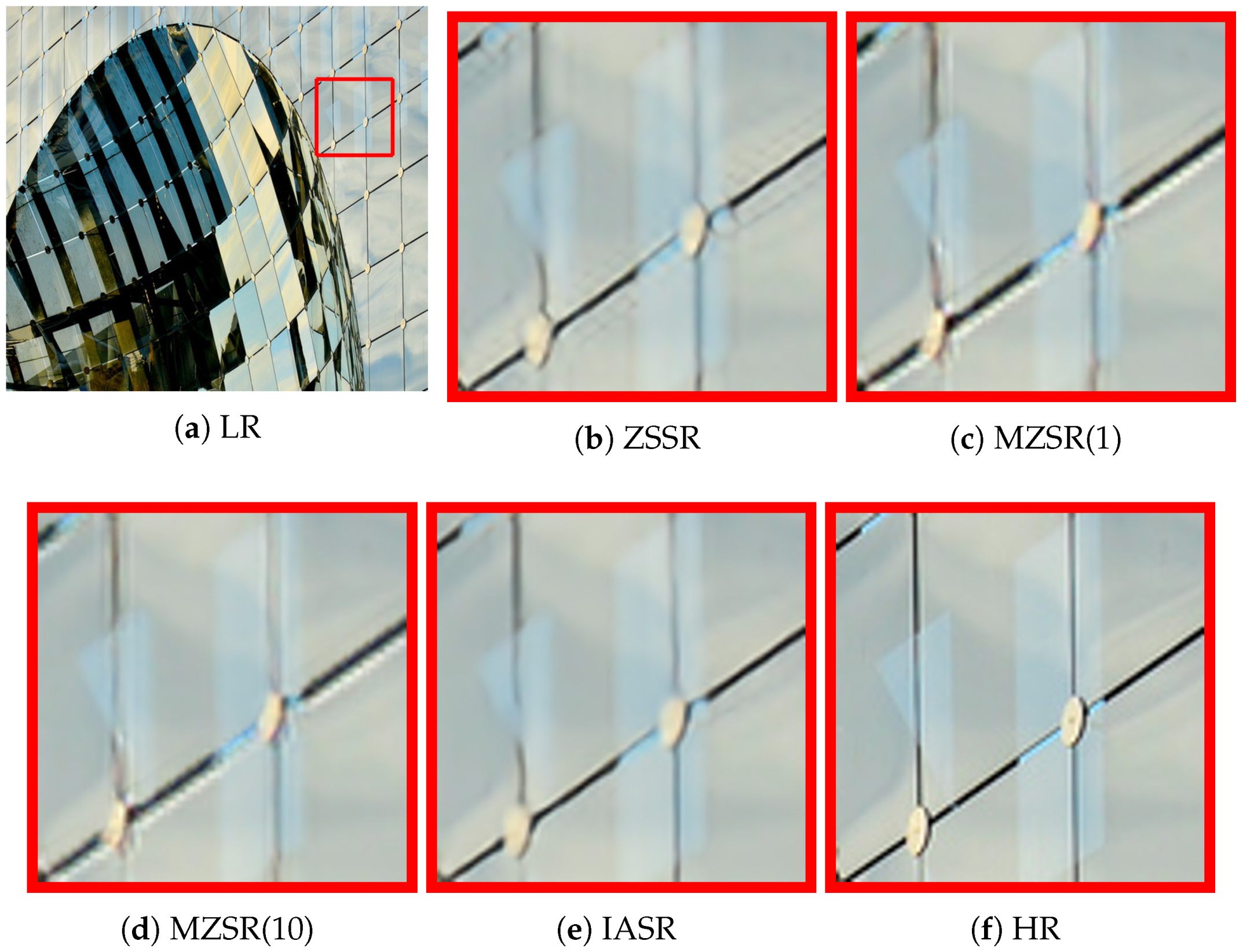
As shown in Figure 4 and Figure 5, IASR yields more accurate details than MZSR and ZSSR, such as straighter window frames and sharper floor gaps.

4.3.2. Evaluations on “Non-Ideal” Case

For the “Non-ideal” case, the experiments are conducted using two downsampling methods with different blur kernels [45]. $g_{\lambda }^b$ refers to isotropic Gaussian blur kernel with width $\lambda$ followed by bicubic downsampling, while $g_{\lambda }^d$ refers to the isotropic Gaussian blur kernel with width $\lambda$ followed by direct downsampling.

For the “direct” downsampling operators, IASR is retrained with the same downsampled LR images, meaning that we trained two models for different downsampling methods: “direct” and “bicubic”. We report the results of $g_{1.3}^b$ and $g_{2.0}^d$ on three benchmarks in

Table 3. The average PSNR/SSIM results on various kernels and downsampling methods with $2\times$ on the benchmarks. The best results are highlighted in red and the second best are in blue.

		No Learning	External Learning		Internal Learning	External and Internal Learning
Kernel	Dataset	Bicubic	RCAN	IKC	ZSSR	MZSR(1)	MZSR(10)	IASR
$g_{1.3}^b$	Set5	30.54	31.54	33.88	35.24	35.18	36.64	35.41
		0.8773	0.8992	0.9357	0.9434	0.9430	0.9498	0.9535
	BSD100	27.49	28.27	30.95	30.74	29.02	31.25	28.92
		0.7546	0.7904	0.8860	0.8743	0.8544	0.8818	0.7563
	Urban100	24.74	25.65	29.47	28.30	28.27	29.83	29.80
		0.7527	0.7946	0.8956	0.8693	0.8771	0.8965	0.8714
$g_{2.0}^d$	Set5	28.73	29.15	29.05	34.90	35.20	36.05	35.48
		0.8449	0.8601	0.8896	0.9397	0.9398	0.9439	0.9403
	BSD100	26.51	26.89	27.46	30.57	30.58	31.09	30.54
		0.7157	0.7394	0.8156	0.8712	0.8627	0.8739	0.8625
	Urban100	23.70	24.14	25.17	27.86	28.23	29.19	28.41
		0.7109	0.7384	0.8169	0.8582	0.8657	0.8838	0.8662

, where RCAN and IKC [46] are supervised methods based on external learning and IKC is recently proposed to estimate blur kernel for blind SR. The performance of the external learning methods trained on the “ideal” case significantly drops when the testing images are not satisfied with the “ideal” case.

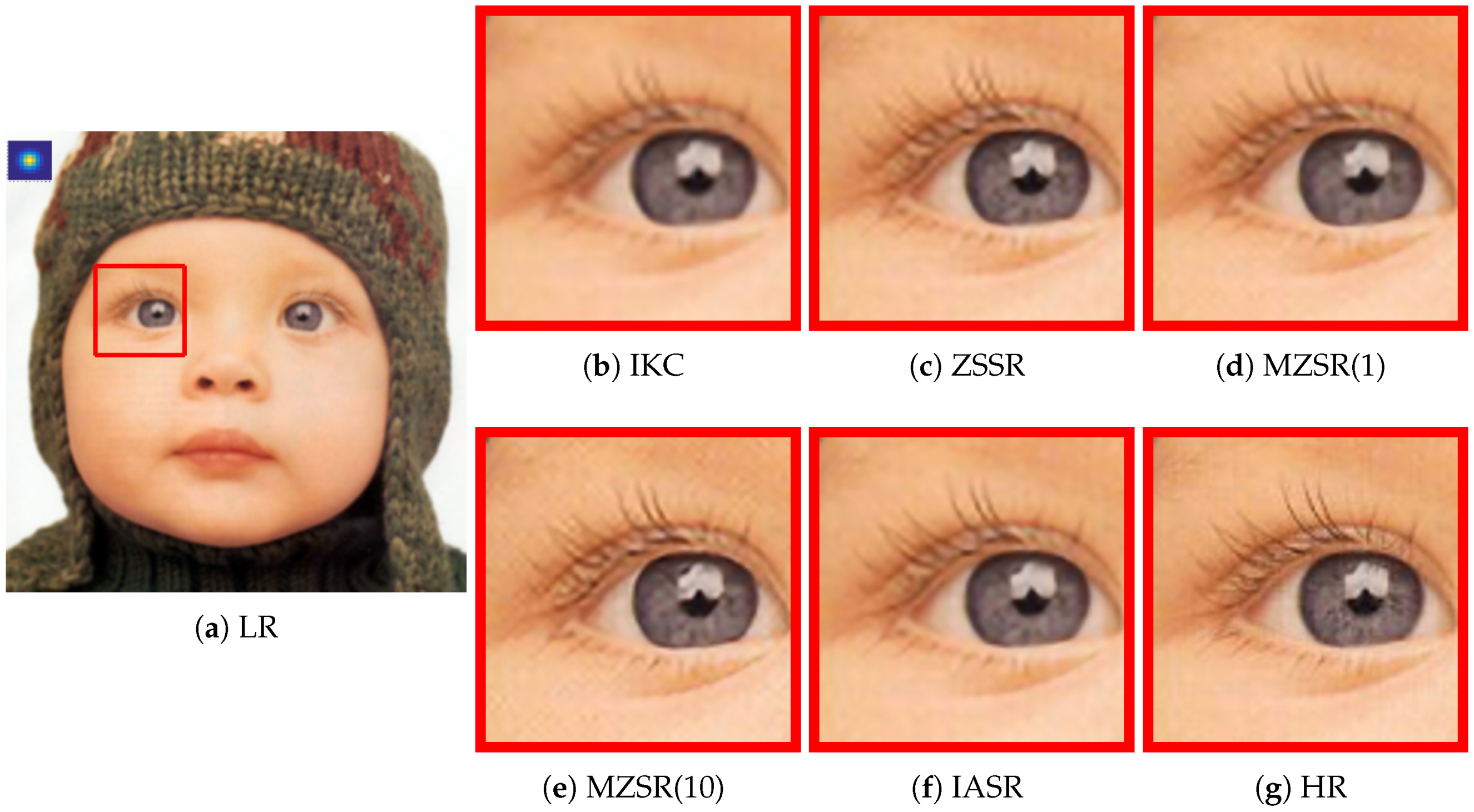
Interestingly, although $N_{ex}$ has never seen the any blurred images, IASR produces comparable results on $g_{1.3}^b$ and $g_{2.0}^d$, and it outperforms both the MSZR(1) and ZSSR on Set5 and Urban100. A visual comparison is present in Figure 6. One can see when the condition is not satisfied with training, both ZSSR and MZSR can restore more details than IKC, and the result of IASR is more consistent with the ground-truth.

4.4. Real Image Super-Resolution

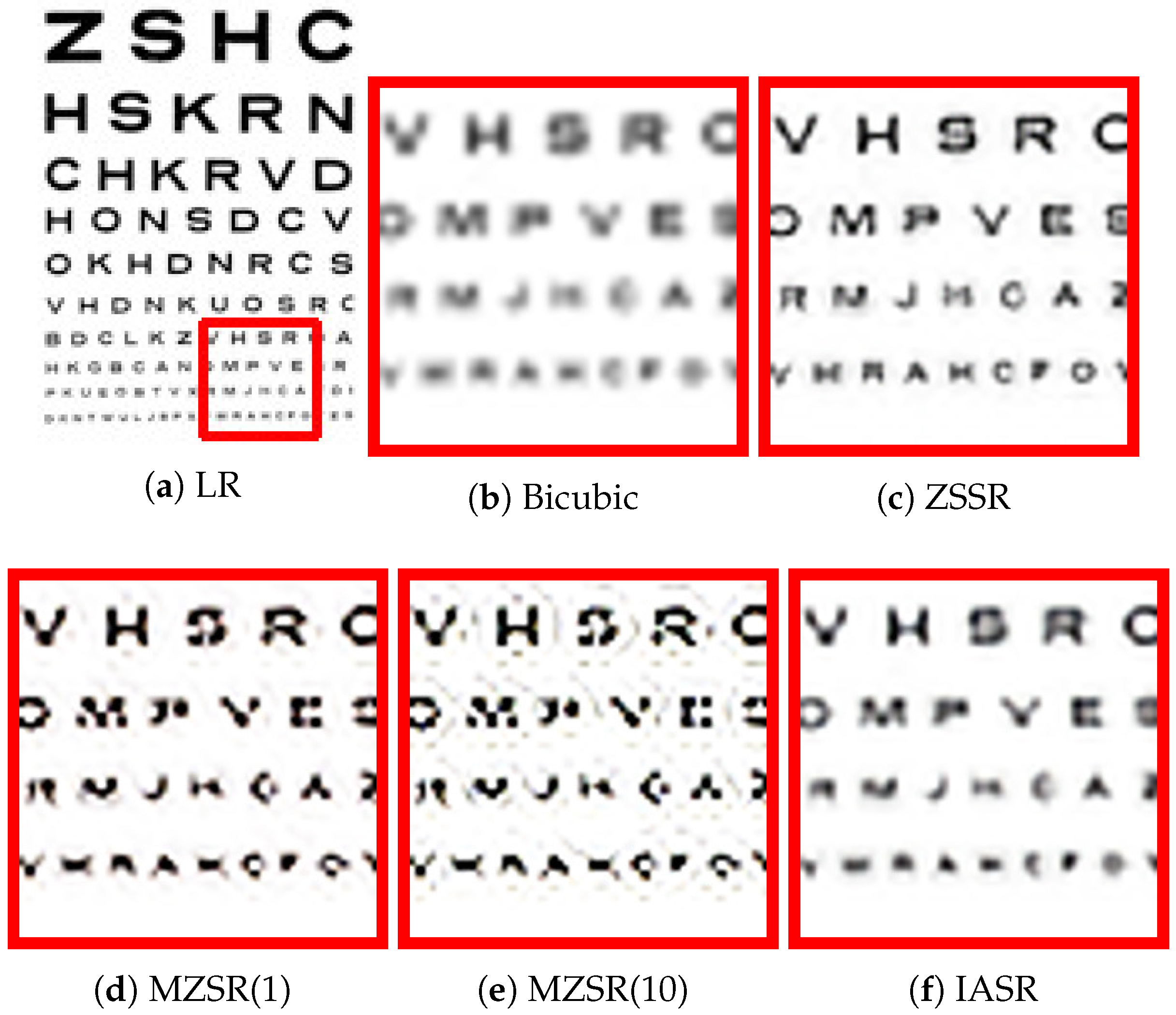
Figure 7 and Figure 8 present the visual comparisons of two real-world examples. The comparison results include the external learning based method ResNet and internal learning based method ZSSR. In the test phase, IASR learns the internal prior solely depending on the test image. The testing LR image is fed to IASR to get the super-resolved image. Figure 7 and Figure 8 show that IASR achieves more visually pleasing results than ResNet and ZSSR. It indicates the robustness of IASR for unknown conditions. For non-reference image reconstruction, the Naturalness Image Quality Evaluator (NIQE) score [46] and BRISQUE [47] are used to measure the quality of the restored image. A smaller NIQE and BRISQUE score indicates better perceptual quality.

Table 4. The NIQE and BRISQUE scores of three real images super-resolution with upscaling factor $2\times$. The best results are highlighted in red and the second best are in blue.

Image	Bicubic	IASR	ZSSR	MZSR(1)	MZSR(10)
Old photo	5.91/42.30	5.88/40.13	6.97/46.79	9.79/85.17	11.39/93.23
Img_005_SRF	6.91/ 42.71	6.04/43.15	6.290/46.18	11.18/91.63	12.67/99.66
Eyechart	15.82/48.99	14.02/48.19	11.68/ 32.23	13.30/ 41.28	14.20/61.84

reports the NIQE and BRISQUE scores of the real image reconstruction results. IASR achieves comparable results of the old photo and the Img_005_SRF, while fails to produce a better result of the eyechart (Figure 9) image than ZSSR.

5. Discussion

5.1. The Kernel Size and Depth of the AFT Layers

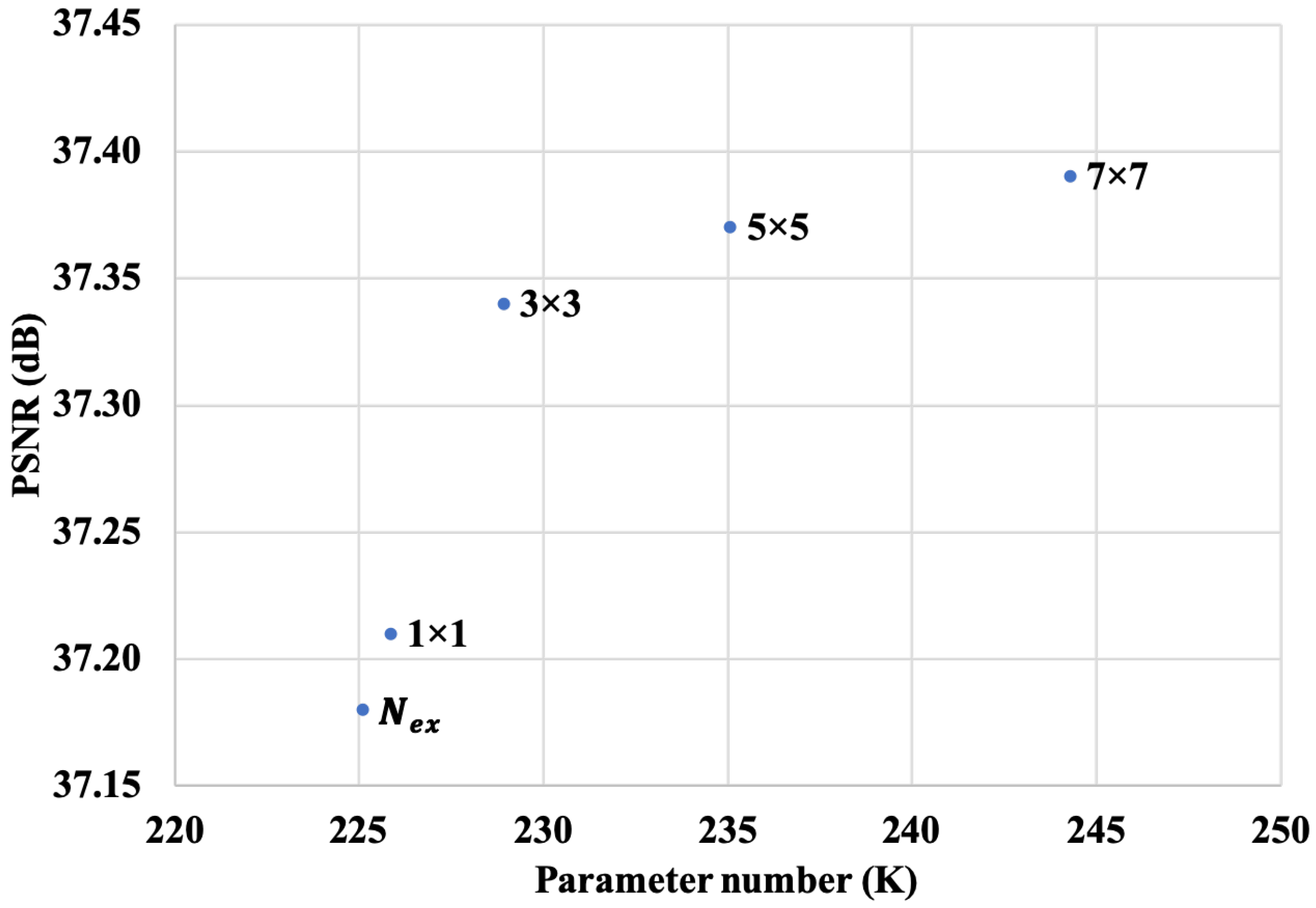
Kernel size and performance. Usually, the larger kernel size tends to improve the SR performance due to better adaptation accuracy. To select a reasonable kernel size, we conduct experiments for the $2\times$ super-resolution task. From the experimental results shown in Figure 10, we observe that gradually increasing the kernel size from $1\times 1$ to $5\times 5$ improves the performance from 37.21 to 37.39 dB, while the number of the parameters increase from 225 to 249 K. Moreover, the performance improvement slows down as the kernel size keeps increasing. The kernel size changing from $5\times 5$ to $7\times 7$ makes little difference, respectively resulting in 37.37 and 32.39 dB when evaluated on Set5. To save computations, we set the kernel size as $3\times 3$ for all AFT layers for all experiments.

Depth and performance. The network goes deeper as more residual blocks are stacked. Figure 11 demonstrates the relation of the number of ResBlock and performance. IASR improves the performance of the basic network $N_{ex}$ as the number of ResBlock increases from one to three. The highest value is achieved when the number of ResBlocks reaches three. When the number is four, we find IASR underperforms the basic network. After that, the performance drops steeply. We suspect that overfitting happens when the limited internal training examples are used in the more complicated model.

5.2. Adapting to the Different Scale Factor

Most of the well-trained CNN-based SR methods are restricted to a fixed scale-factor, meaning that the network can only work well for the same scale during testing. Given LR images with different scales, the performance of the CNN is even worse than that of conventional bicubic interpolation. Figure 1 gives a failed example of CNN-based SR. Since the CNN${}_{4\times }$ is trained on LR images downsampled by a factor of four, it fails to reconstruct a satisfactory HR image when fed an LR image downsampled by a factor of two. One can see that IASR creates visually more pleasing results than ZSSR, which totally depends on internal learning.

Table 5. The PSNRs of different downsampling factors on Set5.

	$\mathbf{2}\mathbf{\downarrow }\mathbf{\to }\mathbf{2}\mathbf{\times }$	$\mathbf{3}\mathbf{\downarrow }\mathbf{\to }\mathbf{2}\mathbf{\times }$	$\mathbf{4}\mathbf{\downarrow }\mathbf{\to }\mathbf{2}\mathbf{\times }$
$N_{ex}$	37.18/0.9571	30.17/0.9042	26.45/0.8277
IASR	37.34/0.9581	35.42/0.9465	35.36/0.9451
Improv.	+0.16/0.0010	+5.25/0.0423	+8.01/0.1174

lists the results of the basic network and IASR for different downsampled LR images. $3\downarrow \to 2\times$ refers to the fact that we train $N_{ex}$ on LR images downsampled by a factor of two while the testing LR image is downsampled by a factor of three. The performance drops by −7.01 and −10.73 dB when $3\downarrow$ and $4\downarrow$ LR images are fed to $N_{ex}$, respectively. On the contrary, IASR produces a more stable performance than $N_{ex}$, which validates its adaptability to the different upscaling factors.

5.3. Complexity Analysis

Memory and time complexities are two critical factors for deep networks. We evaluate several state-of-the-art models on the same PC. The results are shown in

Table 6. Comparisons of the memory and time consumption for the super-resolution of a $256\times 256$ LR image with a scaling factor of $2\times$.

Methods	Parameters	Time (s)
SRCNN	57 K	0.20
VDSR	665 K	0.36
RCAN	15,445 K	1.72
ResNet	225 K	0.33
ZSSR	225 K	148.40
MZSR(1)	225 K	0.13
MZSR(10)	225 K	0.36
IASR	229 K	34.03

.

Memory consumption. Besides the shallow network SRCNN, all three supervised deep models require a large number of parameters. On the contrary, the unsupervised methods only require about one-third of the parameters of VDSR.

Time consumption. To reconstruct an SR image, a fully-supervised network only needs one forward pass. The SRCNN, VDSR and RCAN reconstruct an SR image within two seconds. Internal learning is time expensive because it extracts internal examples and tunes models in the test phase. The runtime depends on the number of internal examples and training stopping criteria. For internal learning, ZSSR stops when its learning rate (starting with 0.001) falls to ${10}^{-6}$ while IASR fixes the number of epochs as 60. Among the unsupervised methods, MZSR with a single gradient update requires the shortest time among the comparison methods. Benefitting from the pre-trained basic model, the convergence speed of IASR is faster than ZSSR, and the average runtime of IASR per image is 34 s for a $256\times 256$ image, which is only $1/4$ of ZSSR. Table 6 reports the time consumption and memory consumption of the different methods.

5.4. Comparison with Other State-of-the-Art Methods

We compare IASR with the other methods that adopt external and internal learning. The relevant three methods perform different strategies for the combination of internal and external learning. Reference [28] synthesized the training data with the additional SR inputs, which were produced by an internal example-driven SISR model; thus, the performances are dependent on the choice of internal example-based SR inputs. To adapt the model to the testing image, Reference [19] performs fine-tuned on the pre-trained deep model, while the performance is lower than other methods. On the contrary, Liang proposed to select the best model from the pre-trained models according to the testing image and then fine-tune the model by the internal example [26]. To perform the model selection strategy effectively, a pool of models must be trained and stored offline, which leads to heavy computation and storage burden. IASR achieves trade-offs between performance and parameter sizes.

Table 7. The average PSNR and memory consumption of different methods which adopt the external and internal learning under the “bicubic” down-sampling scenario on Set5 with $2\times$.

Methods	Parameters	PSNR
IASR	229 K	37.34
[28]	665 K	37.48
[26]	665 K	37.58
[19]	1045 K	36.78

reports the comparison results.

5.5. Limitations and Failed Examples

Figure 11 shows a failed example of IASR. IASR fails to improve the visual quality and tends to blur the result of the pre-trained basic model once there are not enough repetitive pattern occurrences in the LR image. ZSSR recovers more subtle details than ResNet and IASR. We conclude that our method is robust in the case of the same downsampling condition, but it fails to recover image details when the downsampling operator is not consistent with the training phase.

6. Conclusions

In this paper, we proposed a unified framework to integrate external learning and internal learning for image SR. The proposed IASR benefits from a large training dataset via external training, and it implements internal learning during the test phase. We introduce adaptive feature-wise transform layers to learn the internal features’ distribution using examples extracted from the testing LR image and fine-tune the pre-trained network for the given image. IASR boosts the performance of the lightweight model, especially for an image that has strong self-similarities and repetitive patterns. We experimentally determine the appropriate hyper-parameters such as the kernel size and number of blocks to overcome the overfitting issue, and report the limitation of IASR also. In future works, we will focus on how to generalize IASR to different downsampling methods.

References

1. Hou, H.; Andrews, H. Cubic splines for image interpolation and digital filtering. IEEE Trans. Acoust. Speech Signal Process. 1978, 26, 508–517. [Google Scholar]
2. Li, X.; Orchard, M.T. New edge-directed interpolation. IEEE Trans. Image Process. 2001, 10, 1521–1527. [Google Scholar] [PubMed] [Green Version]
3. Irani, M.; Peleg, S. Improving resolution by image registration. CVGIP Graph. Models Image Process. 1991, 53, 231–239. [Google Scholar] [CrossRef]
4. Bevilacqua, M.; Roumy, A.; Guillemot, C.; Morel, M.L.A. Single-image super-resolution via linear mapping of interpolated self-examples. IEEE Trans. Image Process. 2014, 23, 5334–5347. [Google Scholar] [CrossRef] [Green Version]
5. Sun, J.; Xu, Z.; Shum, H.Y. Image super-resolution using gradient profile prior. In Proceedings of the IEEE Conference on Computer Vision and Pattern Recognition (CVPR), Anchorage, AL, USA, 24–26 June 2008; pp. 1–8. [Google Scholar]
6. Yang, C.Y.; Huang, J.B.; Yang, M.H. Exploiting self-similarities for single frame super-resolution. In Proceedings of the Asian Conference on Computer Vision (ACCV), Queenstown, New Zealand, 8–12 November 2010; pp. 497–510. [Google Scholar]
7. Timofte, R.; De Smet, V.; Van Gool, L. Anchored neighborhood regression for fast example-based super-resolution. In Proceedings of the IEEE International Conference on Computer Vision (ICCV), Sydney, Australia, 1–8 December 2013; pp. 1920–1927. [Google Scholar]
8. Shi, Y.; Wang, K.; Xu, L.; Lin, L. Local-and holistic-structure preserving image super resolution via deep joint component learning. In Proceedings of the IEEE International Conference on Multimedia and Expo (ICME), Seattle, WA, USA, 11–15 July 2016; pp. 1–6. [Google Scholar]
9. Liang, Y.; Wang, J.; Zhou, S.; Gong, Y.; Zheng, N. Incorporating image priors with deep convolutional neural networks for image super-resolution. Neurocomputing 2016, 194, 340–347. [Google Scholar] [CrossRef] [Green Version]
10. Huang, J.J.; Liu, T.; Luigi Dragotti, P.; Stathaki, T. SRHRF+: Self-example enhanced single image super-resolution using hierarchical random forests. In Proceedings of the IEEE Conference on Computer Vision and Pattern Recognition Workshops (CVPRW), Honolulu, HI, USA, 21–26 July 2017; pp. 71–79. [Google Scholar]
11. Shocher, A.; Cohen, N.; Irani, M. “Zero-shot” super-resolution using deep internal learning. In Proceedings of the IEEE/CVF Conference on Computer Vision and Pattern Recognition (CVPR), Salt Lake City, UT, USA, 18–22 June 2018; pp. 3118–3126. [Google Scholar]
12. Dong, C.; Loy, C.C.; He, K.; Tang, X. Image super-resolution using deep convolutional networks. In Proceedings of the IEEE Conference on Computer Vision and Pattern Recognition (CVPR), Zurich, Switzerland, 6–12 September 2014; pp. 184–199. [Google Scholar]
13. Dong, C.; Loy, C.C.; He, K.; Tang, X. Image super-resolution using deep convolutional networks. IEEE Trans. Pattern Anal. Mach. Intell. 2016, 38, 295–307. [Google Scholar] [CrossRef] [Green Version]
14. Lim, B.; Son, S.; Kim, H.; Nah, S.; Lee, K.M. Enhanced deep residual networks for single image super-resolution. In Proceedings of the IEEE Conference on Computer Vision and Pattern Recognition Workshops (CVPRW), Honolulu, HI, USA, 21–26 July 2017; pp. 136–144. [Google Scholar]
15. Lai, W.S.; Huang, J.B.; Ahuja, N.; Yang, M.H. Deep Laplacian Pyramid Networks for Fast and Accurate Super-Resolution. In Proceedings of the IEEE Conference on Computer Vision and Pattern Recognition (CVPR), Honolulu, HI, USA, 22–25 July 2017; pp. 624–632. [Google Scholar]
16. Lai, W.S.; Huang, J.B.; Ahuja, N.; Yang, M.H. Fast and Accurate Image Super-Resolution with Deep Laplacian Pyramid Networks. IEEE Trans. Pattern Anal. Mach. Intell. 2018, 41, 2599–2613. [Google Scholar] [CrossRef] [Green Version]
17. Wang, Z.; Chen, J.; Hoi, S.C. Deep learning for image super-resolution: A survey. arXiv 2019, arXiv:1902.06068. [Google Scholar] [CrossRef] [Green Version]
18. Anwar, S.; Khan, S.; Barnes, N. A deep journey into super-resolution: A survey. arXiv 2019, arXiv:1904.07523. [Google Scholar]
19. Wang, Z.; Yang, Y.; Wang, Z.; Chang, S.; Han, W.; Yang, J.; Huang, T. Self-tuned deep super resolution. In Proceedings of the IEEE Conference on Computer Vision and Pattern Recognition Workshops (CVPRW), Boston, MA, USA, 7–12 June 2015; pp. 1–8. [Google Scholar]
20. Freedman, G.; Fattal, R. Image and video upscaling from local self-examples. ACM Trans. Graph. TOG 2011, 30, 1–11. [Google Scholar] [CrossRef] [Green Version]
21. Glasner, D.; Bagon, S.; Irani, M. Super-resolution from a single image. In Proceedings of the IEEE Conference on Computer Vision (CVPR), Kyoto, Japan, 29 September–2 October 2009; pp. 349–356. [Google Scholar]
22. Zhang, J.; Zhao, D.; Gao, W. Group-based sparse representation for image restoration. IEEE Trans. Image Process. 2014, 23, 3336–3351. [Google Scholar] [CrossRef] [PubMed] [Green Version]
23. Ulyanov, D.; Vedaldi, A.; Lempitsky, V. Deep image prior. In Proceedings of the IEEE/CVF Conference on Computer Vision and Pattern Recognition (CVPR), Salt Lake City, UT, USA, 18–22 June 2018; pp. 9446–9454. [Google Scholar]
24. Yokota, T.; Hontani, H.; Zhao, Q.; Cichocki, A. Manifold Modeling in Embedded Space: A Perspective for Interpreting “Deep Image Prior”. arXiv 2019, arXiv:1908.02995. [Google Scholar]
25. Timofte, R.; Rothe, R.; Van Gool, L. Seven Ways to Improve Example-Based Single Image Super Resolution. In Proceedings of the IEEE Conference on Computer Vision and Pattern Recognition (CVPR), Las Vegas, NV, USA, 26 June–1 July 2016; pp. 1865–1873. [Google Scholar]
26. Liang, Y.; Timofte, R.; Wang, J.; Gong, Y.; Zheng, N. Single image super resolution-when model adaptation matters. arXiv 2017, arXiv:1703.10889. [Google Scholar]
27. Wang, Z.; Yang, Y.; Wang, Z.; Chang, S.; Yang, J.; Huang, T.S. Learning super-resolution jointly from external and internal examples. IEEE Trans. Image Process. 2015, 24, 4359–4371. [Google Scholar] [CrossRef] [PubMed]
28. Cheong, J.Y.; Park, I.K. Deep CNN-based super-resolution using external and internal examples. IEEE Signal Process. Lett. 2017, 24, 1252–1256. [Google Scholar] [CrossRef]
29. Li, Z.; Hoiem, D. Learning without forgetting. IEEE Trans. Pattern Anal. Mach. Intell. 2017, 40, 2935–2947. [Google Scholar] [CrossRef] [Green Version]
30. Perez, E.; Strub, F.; De Vries, H.; Dumoulin, V.; Courville, A. FiLM: Visual reasoning with a general conditioning layer. In Proceedings of the AAAI Conference on Artificial Intelligence (AAAI), New Orleans, LA, USA, 2–7 February 2018; pp. 3942–3951. [Google Scholar]
31. Tseng, H.Y.; Lee, H.Y.; Huang, J.B.; Yang, M.H. Cross-Domain Few-Shot Classification via Learned Feature-Wise Transformation. arXiv 2020, arXiv:2001.08735. [Google Scholar]
32. Ulyanov, D.; Vedaldi, A.; Lempitsky, V. Instance normalization: The missing ingredient for fast stylization. arXiv 2016, arXiv:1607.08022. [Google Scholar]
33. Isola, P.; Zhu, J.Y.; Zhou, T.; Efros, A.A. Image-to-image translation with conditional adversarial networks. In Proceedings of the IEEE Conference on Computer Vision and Pattern Recognition Workshops (CVPRW), Honolulu, HI, USA, 21–26 July 2017; pp. 1125–1134. [Google Scholar]
34. Huang, X.; Belongie, S. Arbitrary style transfer in real-time with adaptive instance normalization. In Proceedings of the IEEE International Conference on Computer Vision (ICCV), Venice, Italy, 22–29 October 2017; pp. 1501–1510. [Google Scholar]
35. He, J.; Dong, C.; Qiao, Y. Modulating image restoration with continual levels via adaptive feature modification layers. In Proceedings of the IEEE Conference on Computer Vision and Pattern Recognition (CVPR), Long Beach, CA, USA, 15–21 June 2019; pp. 11056–11064. [Google Scholar]
36. Timofte, R.; Gu, S.; Wu, J.; Van Gool, L. NTIRE 2018 challenge on single image super-resolution: Methods and results. In Proceedings of the IEEE/CVF Conference on Computer Vision and Pattern Recognition (CVPR), Salt Lake City, UT, USA, 18–22 June 2018; pp. 852–863. [Google Scholar]
37. Yang, J.; Wright, J.; Huang, T.; Ma, Y. Image super-resolution as sparse representation of raw image patches. In Proceedings of the IEEE Conference on Computer Vision and Pattern Recognition (CVPR), Anchorage, AK, USA, 24–26 June 2008; pp. 1–8. [Google Scholar]
38. Kingma, D.P.; Ba, J. Adam: A method for stochastic optimization. arXiv 2014, arXiv:1412.6980. [Google Scholar]
39. Paszke, A.; Gross, S.; Chintala, S.; Chanan, G.; Yang, E.; DeVito, Z.; Lin, Z.; Desmaison, A.; Antiga, L.; Lerer, A. Automatic Differentiation in PyTorch. 2017. Available online: https://openreview.net/pdf/25b8eee6c373d48b84e5e9c6e10e7cbbbce4ac73.pdf (accessed on 12 December 2017).
40. Yang, J.; Wright, J.; Huang, T.S.; Ma, Y. Image super-resolution via sparse representation. IEEE Trans. Image Process. 2010, 19, 2861–2873. [Google Scholar] [CrossRef]
41. Martin, D.; Fowlkes, C.; Tal, D.; Malik, J. A database of human segmented natural images and its application to evaluating segmentation algorithms and measuring ecological statistics. In Proceedings of the IEEE International Conference on Computer Vision (ICCV), Vancouver, BC, Canada, 7–14 July 2001; pp. 416–423. [Google Scholar]
42. Huang, J.B.; Singh, A.; Ahuja, N. Single image super-resolution from transformed self-exemplars. In Proceedings of the IEEE Conference on Computer Vision and Pattern Recognition (CVPR), Boston, MA, USA, 7–12 June 2015; pp. 5197–5206. [Google Scholar]
43. Kim, J.; Lee, J.K.; Lee, K.M. Accurate image super-resolution using very deep convolutional networks. arXiv 2015, arXiv:1511.04587. [Google Scholar]
44. Zhang, Y.; Li, K.; Li, K.; Wang, L.; Zhong, B.; Fu, Y. Image super-resolution using very deep residual channel attention networks. In Proceedings of the European Conference on Computer Vision (ECCV), Munich, Germany, 8–14 September 2018; pp. 286–301. [Google Scholar]
45. Soh, J.W.; Cho, S.; Cho, N.I. Meta-Transfer Learning for Zero-Shot Super-Resolution. In Proceedings of the IEEE/CVF Conference on Computer Vision and Pattern Recognition, Virtual, Seattle, WA, USA, 16–18 June 2020; pp. 3516–3525. [Google Scholar]
46. Gu, J.; Lu, H.; Zuo, W.; Dong, C. Blind super-resolution with iterative kernel correction. In Proceedings of the IEEE Conference on Computer Vision and Pattern Recognition (CVPR), Long Beach, CA, USA, 15–21 June 2019; pp. 1604–1613. [Google Scholar]
47. Mittal, A.; Soundararajan, R.; Bovik, A.C. Making a “completely blind” image quality analyzer. IEEE Signal Process. Lett. 2012, 20, 209–212. [Google Scholar] [CrossRef]
Figure 1. Visual comparisons between different methods for 4 × SR on Bird. The super-resolution convolutional neural network (SRCNN) is trained for the low-resolution (LR) image downsampled by a factor of 4. Given an LR image downsampled with a factor of 2, the SRCNN produces over-sharp results. Zero-shot super-resolution (ZSSR) [11] fails to reconstruct pleasant visual details. Image-adaptive super-resolution (IASR) learns the internal prior from an LR image based on the pre-trained SRCNN and creates better results.
Symmetry 12 01686 g001
Figure 2. The overall image-adaptive super-resolution (IASR) scheme. IASR consists of two parts, the basic network ( N e x ) and adaptive feature transformation layers (AFT). (a) External learning. N e x is a residual network, consisting of a residual block with parameters Θ e x , is trained on large external databases at first. (b) Internal learning. We build an internal training dataset based on the test image I l , and then optimize the parameters Θ i n of AFT to learn the internal prior from internal examples while freezing the parameters Θ e x of N e x . Finally, the test image I l is fed into IASR to produce its HR output.
Symmetry 12 01686 g002
Figure 3. The architecture of image-adaptive super-resolution. IASR is composed of a sequence of residual blocks. The difference between the traditional residual block and IASR’s residual block is that IASR’s residual block is integrated with AFT layers.
Symmetry 12 01686 g003
Figure 4. Visual comparisons of different algorithms results ( 3 × ). IASR produces straighter lines along with window frames than ZSSR and MSZR.
Symmetry 12 01686 g004
Figure 5. Visual comparisons of different algorithms results ( 2 × ). Compared with ZSSR and MSZR, IASR recovers sharper floor gaps and less artificial results around the pilot.
Symmetry 12 01686 g005
Figure 6. Visualized comparisons of super-resolution results 2 × with g 1.3 b .
Symmetry 12 01686 g006
Figure 7. Visual comparisons of SR methods for 2× SR for an old landscape photo downloaded from the Internet.
Symmetry 12 01686 g007
Figure 8. Visual comparisons of the SR methods for 2× SR on a real-world image. (ae) refer to the results of Bicubic, ZSSR, MZRR(1), MZSR(10) and IASR respectively. The original image was downloaded from the “ZSSR” project website.
Symmetry 12 01686 g008
Figure 9. Failed example. Due to the unknown downsampling method, IASR produces fewer details than ZSSR and MSZR for the last two lines of the eyechart.
Symmetry 12 01686 g009
Figure 10. The performances of the different filter sizes of the AFT layers (Set5 2 × ).
Symmetry 12 01686 g010
Figure 11. The performances of the different depths of AFT layers (Set5 2 × ).
Symmetry 12 01686 g011