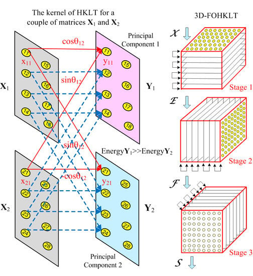
Article

Complexity Estimation of Cubical Tensor Represented through 3D Frequency-Ordered Hierarchical KLT

by
Roumen Kountchev
1,*,
Rumen Mironov
1 and
Roumiana Kountcheva
2
1
Faculty of Telecommunications, Department Radio Communications and Video Technologies, Technical University of Sofia, 1000 Sofia, Bulgaria
2
TK Engineering, 1582 Sofia, Bulgaria
*
Author to whom correspondence should be addressed.
Symmetry 2020, 12(10), 1605; https://doi.org/10.3390/sym12101605
Submission received: 6 August 2020 / Revised: 22 September 2020 / Accepted: 25 September 2020 / Published: 26 September 2020
(This article belongs to the Special Issue Advances in Symmetric Tensor Decomposition Methods)

Abstract

:
In this work is introduced one new hierarchical decomposition for cubical tensor of size 2n, based on the well-known orthogonal transforms Principal Component Analysis and Karhunen–Loeve Transform. The decomposition is called 3D Frequency-Ordered Hierarchical KLT (3D-FOHKLT). It is separable, and its calculation is based on the one-dimensional Frequency-Ordered Hierarchical KLT (1D-FOHKLT) applied on a sequence of matrices. The transform matrix is the product of n sparse matrices, symmetrical at the point of their main diagonal. In particular, for the case in which the angles which define the transform coefficients for the couples of matrices in each hierarchical level of 1D-FOHKLT are equal to π/4, the transform coincides with this of the frequency-ordered 1D Walsh–Hadamard. Compared to the hierarchical decompositions of Tucker (H-Tucker) and the Tensor-Train (TT), the offered approach does not ensure full decorrelation between its components, but is close to the maximum. On the other hand, the evaluation of the computational complexity (CC) of the new decomposition proves that it is lower than that of the above-mentioned similar approaches. In correspondence with the comparison results for H-Tucker and TT, the CC decreases fast together with the increase of the hierarchical levels’ number, n. An additional advantage of 3D-FOHKLT is that it is based on the use of operations of low complexity, while the similar famous decompositions need large numbers of iterations to achieve the coveted accuracy.

Graphical Abstract

1. Introduction

The well-known tensor decompositions Canonical Polyadic Decomposition (CPD), Higher-Order Singular Value Decomposition (HOSVD) [1,2,3], Tensor Train (TT) Decomposition [4], Hierarchical Tucker decomposition (H-Tucker) [5] and some of their modifications [6,7] are based on the calculation of the eigenvalues and eigenvestors of the decomposed tensor. The basic attribute of this group is that they are optimal regarding the minimization of the mean square approximation error derived from the “truncation” of the low-energy components. For the calculation of the retained components, we use iterative methods which need relatively large numbers of mathematical operations to achieve the requested accuracy (Power method [8], Jacoby method [9], etc.).
The hierarchical tensor decompositions based on the H-Tucker algorithm are generalized in publications [7] and [10]. In [7], Vasilescu and Kim introduced a compositional hierarchical tensor factorization that disentangles the hierarchical causal structure of object image formation, but the computational complexity (CC) of the method is not evaluated. In [10], Zniyed et al. offered the TT-based hierarchical decomposition of high-order tensors, for the calculation of which is used the Tensor-Train Hierarchical SVD (TT-HSVD). This approach permits parallel processing, which accelerates the calculations. Unlike the TT-SVD algorithm, the TT-HSVD is based on applying SVDs to matrices of smaller dimensions. As a result, the CC of TT-SVD is O(R2N3) operations higher than that of TT-HSVD (here, R is the rank of the hypercubical tensor of size N).
As an alternative, in this work are presented new hierarchical 3D tensor decompositions, based on the famous statistical orthogonal transforms Principal Component Analysis (PCA) and the Karhunen–Loeve Transform (KLT) [11,12]. The offered decompositions are close to the optimal (which ensure full decorrelation of their components), but do not need iterations and have low computational complexity.
In Section 2, we present the methods for one-dimensional hierarchical adaptive transform based on the PCA (1D-HAPCA) and the Hierarchical Adaptive Karhunen–Loeve Transform (1D-HAKLT). In Section 3, on the basis of these 1D transforms we give the details of the cubical tensor decomposition through separable 3D Frequency-Ordered Hierarchical KLT (3D-FOHKLT), and Section 4 contains the related algorithm. Section 5 presents the comparative analysis of the computational complexity of the new approaches with respect to the well-known hierarchical Tucker decomposition (H-Tucker) and the TT decomposition. Section 6 is the Conclusion.

2. One-Dimensional Hierarchical Adaptive PCA/KLT Transform for a Sequence of Matrices

The detailed description of the algorithm for the one-dimensional adaptive PCA/KLT transform (1D-APCA/AKLT) for a couple of matrices is given below. This is the basis of the hierarchical algorithm for processing the sequence of matrices which represent the corresponding tensor.
Throughout this paper, scalars are represented as x, vectors and matrices as x and X correspondingly, and tensors as X . It is also assumed here that all tensor elements (entries) are nonnegative real numbers x(i,j,k).

2.1. One-Dimensional Adaptive PCA/KLT Transform for a Sequence of Matrices

The transform is executed in the following way.
First, on the elements x1s and x2s, which have the same spatial position in the couple of matrices X1 and X2 of size N × N, are applied one-dimensional direct and inverse adaptive PCA, i.e., the 1D-APCA [12] is:
y 1 s = ( x 1 s m 1 ) cos θ 1 , 2 + ( x 2 s m 2 ) sin θ 1 , 2 ; y 2 s = ( x 1 s m 1 ) sin θ 1 , 2 ( x 2 s m 2 ) cos θ 1 , 2 ; x 1 s = y 1 s cos θ 1 , 2 + y 2 s sin θ 1 , 2 + m 1 ; x 2 s = y 1 s sin θ 1 , 2 y 2 s cos θ 1 , 2 + m 2 , for s = 1 , 2 , , N 2
Here, y1s and y2s are the corresponding elements in the couple of transformed matrices Y1 and Y2, each of size N × N,
θ 1 , 2 = arctg { 2 k 3 / ( k 1 k 2 + ( k 1 k 2 ) 2 + 4 k 3 2 ) } ;
k 1 = E ( x 1 s 2 ) m 1 2 , k 2 = E ( x 2 s 2 ) m 2 2 , k 3 = E ( x 1 s x 2 s ) m 1 m 2 ;
m 1 = E ( x 1 s ) , m 2 = E ( x 2 s ) ,
where m = E ( x s ) = ( 1 / N 2 ) s = 1 N 2 x s is the averaging operator.
To calculate the angle θ1,2 it is necessary to define the extended arctg function. If β2 = 2k3 and β 1 = k 1 k 2 + ( k 1 k 2 ) 2 + 4 k 3 2 are two real numbers, the extended arctg function εarctg1, β2) is mapped to (−π, π] by adding π [13]:
ε arctg ( β 1 , β 2 ) = arctg ( β 2 / β 1 ) ,   if   β 1 > 0 ; arctg ( β 2 / β 1 ) + π ,   if   β 1 < 0 ,   β 2 0 ; arctg ( β 2 / β 1 ) π ,   if   β 1 < 0 , β 2 < 0 ; π / 2 ,   if   β 1 = 0 ,   β 2 > 0 ; π / 2 ,   if   β 1 = 0 , β 2 < 0 ; 0 ,   if   β 2 = β 1 = 0 .
In particular, for m 1 = m 2 = 0 (valid for 1D-AKLT) and θ 1 , 2 = π / 4 , the relations (1) become as follows:
y 1 s = ( 1 / 2 ) ( x 1 s + x 2 s ) ; y 2 s = ( 1 / 2 ) ( x 1 s x 2 s ) ; x 1 s = ( 1 / 2 ) ( y 1 s + y 2 s ) ; x 2 s = ( 1 / 2 ) ( y 1 s y 2 s ) .
Hence, in this case the 1D-KLT coincides with the 1D Walsh–Hadamard Transform (1D-WHT).

2.2. One-Dimensional Hierarchical Adaptive KLT for a Sequence of Matrices

The relations above, used for the calculation of 1D-APCA [12], are the kernel for the processing of a sequence of matrices (for example, a sequence of moving images), and do not need iterative calculations. The procedure is executed in the following way. First, the sequence of matrices Xk, each of size N × N for k = 1, 2,…, N is divided into N/2 couples (N = 2n). For each couple of matrices with elements x1s(p,q) and x2s(p,q), when q = 1, 2, …, N/2, in the level p = 1, 2, …, n, is executed the one-dimensional adaptive PCA (1D-APCA), in accordance with Equations (1)–(5). For m 1 ( p , q ) = m 2 ( p , q ) = 0 (valid for the KLT), the direct 1D-AKLT for the couple of matrices q in the level p of the 1D-HAKLT is defined by the relations
y 1 s ( p , q ) = x 1 s ( p , q ) cos θ p , q + x 2 s ( p , q ) sin θ p , q y 2 s ( p , q ) = x 1 s ( p , q ) sin θ p , q x 2 s ( p , q ) cos θ p , q   for   s =   1 ,   2 ,   ,   N 2 ,
where s is the sequential number of two elements of the same position in the couple of matrices, q,
θ p , q = arctg { 2 k 3 ( p , q ) / [ k 1 ( p , q ) k 2 ( p , q ) + ( k 1 ( p , q ) k 2 ( p , q ) ) 2 + 4 k 3 2 ( p , q ) ] } , k 1 ( p , q ) = E ( x 1 s 2 ( p , q ) ) ; k 2 ( p , q ) = E ( x 2 s 2 ( p , q ) ) ; k 3 ( p , q ) = E ( x 1 s ( p , q ) x 2 s ( p , q ) ) .
In the equations, figures and text below are introduced the following symbols: cos θ p , q = c p , q and sin θ p , q = s p , q for p = 1, 2, 3 and q = 1, 2, 3, 4. The execution graph for 1D-HAKLT of three hierarchical levels (N = 8) is shown on Figure 1a. In every level p = 1, 2, 3, and for each couple of neighbor matrices q (fenced in red ellipses) 1D-APCA is executed. In result, the first transformed matrix calculated for each couple q has higher energy than the second matrix, and they are mutually decorrelated. To continue with the operations in the next level of 1D-HAKLT, these matrices are reordered, following the decrease of their energy, i.e.,
P Y p , 0 P Y p , 1 P Y p , 2 P Y p , k P Y p , 7 ,
where P Y p , k = i = 1 8 j = 1 8 [ y p , k ( i , j ) ] 2 is the energy of matrices Yp,k with elements y p . k ( i , j ) , obtained in result of the execution of 1D-HAKLT in levels p = 1, 2, 3, before the reordering. In result, the reordered matrices Er in the last level are decorrelated to the highest degree [12].
The reordering in each level p in accordance with Equation (9) needs significant computational resources. For the case when the connections between the outputs Yp,k for k = 1, 2, …, 8 in the level p and the inputs in the next level p + 1 are fixed, reordering is not performed, and the 1D-HAKLT turns into the one-dimensional Frequency-Ordered Hierarchical KLT (1D-FOHKLT), whose execution graph is shown in Figure 1b. In this case, only the output matrices in the last (third) level are reordered, which does not require mathematical operations. Besides, the energy distribution of matrices Yp,k is close to that defined by Equation (9). In particular, in accordance with Appendix A, if θ p , q = π / 4 for p = 1, 2, 3 and q = 1, 2, 3, 4, then 1D-HAKLT coincides with the one-dimensional frequency-ordered Fast Walsh–Hadamard Transform (1D-FWHT) for N = 8 [14].
Both algorithms are generalized below for N = 2n. The algorithm for fast hierarchical 1D-HAKLT is represented through the sequential transformation of the vectors’ elements s in each decomposition level p, in accordance with the relations
y 1 , s = P 1 ( 2 n ) G 1 ( 2 n ) x s for   p = 1   and   s = 1 , 2 , , N 2 ;
y p , s = P p ( 2 n ) G p ( 2 n ) y p 1 , s for   p = 2 , 3 , , n 1   and   s = 1 , 2 , , N 2 ;
e s = P n ( 2 n ) G n ( 2 n ) y n 1 , s . for p = n   and   s = 1 , 2 , , N 2 .
Here, xs and es are respectively the input and the output column-vector of N components correspondingly, and the column-vectors yp,s for p = 2, 3,…, n − 1 are the intermediate results. The relation between vectors es and xs, defined on the basis of Equations (10)–(12), is given below:
e s = [ p = 1 n P p ( 2 n ) G p ( 2 n ) ] x s = T HAKLT ( 2 n ) x s   for   s =   1 , 2 ,   , N 2 ,
where
T HAKLT ( 2 n ) = p = 1 n P p ( 2 n ) G p ( 2 n )
is the matrix for the fast n-level 1D-HAKLT. The sparse transform matrices G p ( 2 n ) of size 2n × 2n have a symmetrical block-diagonal structure towards the main diagonal, and are defined by the relations
G p ( 2 n ) = q = 1 2 n 1 T p , q ( 2 ) = diag { T p , 1 ( 2 ) , T p , 2 ( 2 ) , , T p , 2 n 1 ( 2 ) }   for   p = 1 ,   2 ,   ,   n ,
where T p , q ( 2 ) = c p , q s p , q s p , q c p , q , and ⊕ denotes the direct sum of matrices. The permutation matrices P p ( 2 n ) of size 2n × 2n for level p = 1, 2, …, n of 1D-HAKLT are defined on the basis of Equation (9) for k = 0, 1, 2, …, 2n−1.
The algorithm 1D-FOHKLT is depicted by a relation similar to Equation (13), but the reordering is executed only in the last level, n;
e s = P n ( 2 n ) [ p = 1 n G p ( 2 n ) ] x s = T FOHKLT ( 2 n ) x s   for   s =   1 ,   2 ,   ,   N 2 ,
where T FOHKLT ( 2 n ) = P n ( 2 n ) [ p = 1 n G p ( 2 n ) ] is the matrix for 1D-FOHKLT, P n ( 2 n ) is the permutation matrix P n ( 2 n ) for the last level n, and p = 1 n G p ( 2 n ) is the product of n sparse transform matrices G p ( 2 n ) for p = 1, 2, 3, …, n.
Each matrix G p ( 2 n ) is defined as follows:
G p ( 2 n ) = i = 1 2 n p j = 1 2 p 1 c p , 2 p 1 ( i 1 ) + j j = 1 2 p 1 s p , 2 p 1 ( i 1 ) + j j = 1 2 p 1 s p , 2 p 1 ( i 1 ) + j j = 1 2 p 1 c p , 2 p 1 ( i 1 ) + j   for   p = 1 ,   2 ,   3 , ,   n ,
where
i = 1 2 n p j = 1 2 p 1 c p , 2 p 1 ( i 1 ) + j j = 1 2 p 1 s p , 2 p 1 ( i 1 ) + j j = 1 2 p 1 s p , 2 p 1 ( i 1 ) + j j = 1 2 p 1 c p , 2 p 1 ( i 1 ) + j = j = 1 2 p 1 c p , j j = 1 2 p 1 s p , j j = 1 2 p 1 s p , j j = 1 2 p 1 c p , j j = 1 2 p 1 c p , 2 p 1 + j j = 1 2 p 1 s p , 2 p 1 + j j = 1 2 p 1 s p , 2 p 1 + j j = 1 2 p 1 c p , 2 p 1 + j j = 1 2 p 1 c p , 2 p 1 ( n p 1 ) + j j = 1 2 p 1 s p , 2 p 1 ( n p 1 ) + j j = 1 2 p 1 s p , 2 p 1 ( n p 1 ) + j j = 1 2 p 1 c p , 2 p 1 ( n p 1 ) + j .
In the level n are rearranged the components of the column-vectors y n , s = G n ( 2 n ) y n 1 , s , and, respectively, the components of matrices Yn,k for k = 0, 1, …, N − 1. For this is used the permutation matrix P n ( 2 n ) . From the components of the column-vectors e s = P n ( 2 n ) y n , s are obtained the matrices E0, E1, …, EN−1. The frequency-ordered matrices Er are calculated in accordance with the relation between their sequential number r and the corresponding sequential number k, for the matrices Yn,k. The relation which defines the matrix P n ( 2 n ) is as follows [14]:
  • the binary code k n 1 , k n 2 , , k 0 of the sequential decimal number k = 0, 1, …, 2n−1 of the component Yn,k is arranged inversely (i.e., k 0 , k 1 , , k n 1 ), as follows:
    g i = k n i 1   for   0 i n 1 ;
  • the so-obtained code g n 1 , g n 2 , , g 0 is transformed from Gray code into binary code r n 1 , r n 2 , , r 0 , in accordance with the operations
    r n 1 = g n 1 ,   r i = r i 1 g i   for   0 i n 2 .
Here, ⊕ is the symbol for the operation “exclusive OR”. The decimal number r = i = 0 n 1 r i 2 i defines the sequential number of the component Er for r = 0, 1, …,2n−1, which before the rearrangement corresponded to the component Yn,k, with sequential number k = i = 0 n 1 k i 2 i .
An example for the direct 1D-FOHKLT of three hierarchical levels is given in Appendix A.

3. Decomposition of Cubical Tensor of Size N × N × N through 3D-FOHKLT

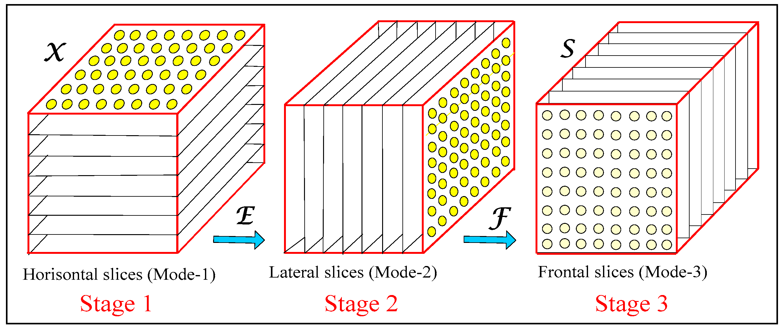
The decomposition 3D-FOHKLT for a cubical tensor X of size 8 × 8 × 8, executed in three consecutive stages, is shown on Figure 2.
In the first stage, the tensor X is divided into eight horizontal slices (mode-1). Then, in accordance with Figure 1, on each couple of matrices is applied 1D-FOHKLT. In result, the sequence of eight transformed matrices is united into one new tensor, E . In the second stage, the input tensor E is divided into eight lateral slices (mode-2), then the couples of matrices are transformed, and after that united into the tensor F . In the third stage, the input tensor F is divided into eight frontal slices (mode-3). After applying the 1D-AKLT on each couple of matrices which build the tensor F , the final result is obtained—the general spectral tensor S , with elements s ( u , v , l ) . The initial tensor X is restored from the tensor S through summation of all “weighted” basic tensors K u , v , l of size 8 × 8 × 8, in accordance with the relation
X = ( 1 / 512 ) [ s 0 , 0 , 0 K 0 , 0 , 0 + s 1 , 0 , 0 K 1 , 0 , 0 + + s 7 , 7 , 7 K 7 , 7 , 7 ] = ( 1 / 8 3 ) u = 0 7 v = 0 7 l = 0 7 s ( u , v , l ) K u , v , l .
Here, s ( u , v , l ) are the weight coefficients of the basic tensor, K u , v , l . Each basic tensor is represented as the outer product of three vectors:
K u , v , l = k u ( 1 ) k v ( 2 ) k l ( 3 ) ,
where o is the symbol for the outer product of the two column-vectors ( x y = x . y T ) and k u ( 1 ) , k v ( 2 ) , k l ( 3 ) are the basic vectors for the first, second and third stages of 3D-FOHKLT, respectively. These vectors are defined by using the matrix T F O H K L T ( 8 ) for 1D-FOHKLT, in accordance with Equation (A6) from Appendix A. The vector k u ( 1 ) for u = 0, 1, …, 7 comprises the elements of the u-th row of the matrix T FOHKLT 1 ( 8 ) for the first stage (t = 1) of 3D-FOHKLT. The vectors k v ( 2 ) and k l ( 3 ) for v, l = 0, 1, …, 7 comprise the elements of rows v and l in the matrices T FOHKLT 2 ( 8 ) and T FOHKLT 3 ( 8 ) for the second (t = 2) and third (t = 3) stages of 3D-FOHKLT, respectively. The basic vectors are defined below for t = 1, 2, 3 and u, v, l = 0, 1, …, 7:
k u ( t ) = [ k u , 1 t , k u , 2 t , k u , 3 t , k u , 4 t , k u , 5 t , k u , 6 t , k u , 7 t , k u , 8 t ] T ;
k v ( t ) = [ k v , 1 t , k v , 2 t , k v , 3 t , k v , 4 t , k v , 5 t , k v , 6 t , k v , 7 t , k v , 8 t ] T ;
k l ( t ) = [ k l , 1 t , k l , 2 t , k l , 3 t , k l , 4 t , k l , 5 t , k l , 6 t , k l , 7 t , k l , 8 t ] T .
The general number of the basic tensors in this case is 83. For example, if u = 3, v = 2 and l = 6, the components of these vectors for each stage are defined by the relations below:
k 3 ( 1 ) = [ k 3 , 0 1 , k 3 , 1 1 , k 3 , 2 1 , k 3 , 3 1 , k 3 , 4 1 , k 3 , 5 1 , k 3 , 6 1 , k 3 , 7 1 ] T = = [ c 3 , 3 1 s 2 , 1 1 c 1 , 1 1 ,   c 3 , 3 1 s 2 , 1 1 s 1 , 1 1 , c 3 , 3 1 c 2 , 1 1 c 1 , 2 1 , c 3 , 3 1 c 2 , 1 1 s 1 , 2 1 , s 3 , 3 1 s 2 , 3 1 c 1 , 3 1 , s 3 , 3 1 s 2 , 3 1 s 1 , 3 1 , s 3 , 3 1 c 2 , 3 1 c 1 , 4 1 , s 3 , 3 1 c 2 , 3 1 s 1 , 4 1 ] T ;
k 2 ( 2 ) = [ k 2 , 1 2 , k 2 , 2 2 , k 2 , 3 2 , k 2 , 4 2 , k 2 , 5 2 , k 2 , 6 2 , k 2 , 7 2 , k 2 , 8 2 ] T = = [ s 3 , 3 2 s 2 , 1 2 c 1 , 1 2 ,   s 3 , 3 2 s 2 , 1 2 s 1 , 1 2 , s 3 , 3 2 c 2 , 1 2 c 1 , 2 2 , s 3 , 3 2 c 2 , 1 2 s 1 , 2 2 , c 3 , 3 2 s 2 , 3 2 c 1 , 3 2 , c 3 , 3 2 s 2 , 3 2 s 1 , 3 2 , c 3 , 3 2 c 2 , 3 2 c 1 , 4 2 , c 3 , 3 2 c 2 , 3 2 s 1 , 4 2 ] T ;
k 6 ( 3 ) = [ k 6 , 1 3 , k 6 , 2 3 , k 6 , 3 3 , k 6 , 4 3 , k 6 , 5 3 , k 6 , 6 3 , k 6 , 7 3 , k 6 , 8 3 ] T = = [ s 3 , 2 3 c 2 , 2 3 s 1 , 1 3 ,   s 3 , 2 3 c 2 , 2 3 c 1 , 1 3 , s 3 , 2 3 s 2 , 2 3 s 1 , 2 3 , s 3 , 2 3 s 2 , 2 3 c 1 , 2 3 , c 3 , 2 3 c 2 , 4 3 s 1 , 3 3 , c 3 , 2 3 c 2 , 4 3 c 1 , 3 3 , c 3 , 2 3 s 2 , 4 3 s 1 , 4 3 , c 3 , 2 3 s 2 , 4 3 c 1 , 4 3 ] T .
The vectors k u ( t ) , k v ( t ) , k l ( t ) are orthonormalized, i.e., for their components are valid the relations:
m = 1 8 k u 1 , m t 1 . k u 2 , m t 2 = 0   for   t 1 t 2 ; 1   for   t 1 = t 2 ,   where   u 1 ,   u 2 = 0 ,   1 ,   ,   7   and   t 1 ,   t 2 = 1 ,   2 ,   3 .
The decomposition 3D-HAKLT, shown in Figure 2, could be easily generalized for the cases when N = 16, 32, …, 2n through uniting the computational principles from Figure 1 and Figure 2 for decompositions of high numbers of levels (n = 4, 5, …). From Equation (29), it follows that the rows of the matrices T FOHKLT t 1 ( 8 ) and T FOHKLT t 2 ( 8 ) for t 1 t 2 are not correlated. This conclusion could also be generalized for the rows of the matrices T FOHKLT t 1 ( 2 n ) and T FOHKLT t 2 ( 2 n ) . Hence, after the execution of each stage of 3D-FOHKLT, the so-calculated N slices in the corresponding direction are highly decorrelated [12,15].
In the general case, the spectral coefficients s(u,v,l) are calculated through direct 3D-KLT, in accordance with the relation
s u , v , l = i = 0 N 1 j = 0 N 1 k = 0 N 1 x i , j , k k a r ( i , u , N ) k a r ( j , v , N ) k a r ( k , l , N )   for   u ,   v ,   l = 0 ,   1 ,   ,   N 1 .
The three-dimensional inverse KLT is defined by the relation
x i , j , k = 1 N 3 u = 0 N 1 v = 0 N 1 l = 0 N 1 s u , v , l k a r ( i , u , N ) k a r ( j , v , N ) k a r ( k , l , N )   for   i ,   j ,   k = 0 ,   1 ,   ,   N 1 .
Here the 1D-Karhunen–Loeve (KL) functions of the Nth order are kar(i,u,N), kar(j,v,N), and kar(k,l,N).
Each third-order tensor X of size N × N × N is represented as the weighted sum of N3 3D-KL functions obtained by using the tensors K u , v , l , each of size N × N × N:
X = ( 1 / N 3 ) [ s 0 , 0 , 0 K 0 , 0 , 0 + s 1 , 0 , 0 K 1 , 0 , 0 + + s N 1 , N 1 , N 1 K N 1 , N 1 , N 1 ] = ( 1 / N 3 ) u = 0 N 1 v = 0 N 1 l = 0 N 1 s ( u , v , l ) K u , v , l .
Then, the tensor decomposition based on the 3D-FOHKLT is defined by the relation
X = ( 1 / N 3 ) u = 0 N 1 v = 0 N 1 l = 0 N 1 s ( u , v , l ) [ k u ( 1 ) k v ( 2 ) k l ( 3 ) ] .
Hence, in this case the tensor X of size N × N × N is decomposed in a way similar to that of the Tucker decomposition [2];
X = r 1 = 1 R r 2 = 1 R r 3 = 1 R d r 1 , r 2 , r 3 ( a r 1 b r 2 c r 3 ) .
Here, d r 1 , r 2 , r 3 are the eigen values of the tensor X , a r 1 , b r 2 , c r 3 are the corresponding eigen vectors, and R is the tensor rank. The rank of the three-way tensor X of size I × J × K is bounded from above in accordance with the inequality, as follows: max { I , J , K } R min { I × J , I × K , J × K } [3]. If I = J = K = N, then N R N 2 . The difference between the decompositions from Equations (33) and (34) is the number of their components, which can reach up to N3 and N2, respectively (for the maximum value of the rank, R). In the case that the decomposition components number as defined by Equation (33) is not reduced, the 3D-HAKLT is reversible, i.e., the coefficients s(u,v,l) of the tensor S and its basic tensors K u , v , l are sufficient to restore the tensor X.

4. Algorithm 3D-FOHKLT for Cubical Tensor Representation

The representation of the tensor X of size N × N × N, through 3D-FOHKLT based on the spectral tensor S , is executed in correspondence with Figure 2. Each stage of the 3D transform is calculated for N = 8 through 1D-FOHKLT, as shown in Figure 1b.
Algorithm 1: Tensor representation based on the 3D-FOHKLT
Input: Third-order tensor X of size N × N × N (N = 2n) and with elements x(i,j,k)
Output: Spectral tensor S of n layers, whose elements s(u,v,l) are the coefficients of the 3D-FOНKLT.
1 begin
2 Divide the tensor X into horisontal slices and compose N/2 couples of matrices X p , q 1 and X p , q 2 of size
  N × N, for q = 1, 2, …, N/2;
3 for each couple of matrices X p , q 1 and X p , q 2 when q = 1, 2, …, N/2 and p = 1, 2, …, n, do
4   Calculate the couple of matrices Y p , q 1 and Y p , q 2 obtained through 1D-FOНKLT in
     accordance with Equations (7) and (8);
5   Calculate the matrices P n ( 2 n ) and Yn,k for k = 0, 1, …, N−1 and p = n in accordance with Equations (18)–(20);
6   Define the matrices Er for r = 0, 1, …, N−1 in the level p = n by rearranging the matrices Yn,k for
     k = 0, 1, …, N−1 on the basis of the vector transform e s = P n ( 2 n ) y n , s , for s = 1, 2, …, N2;
7   Reshape all rearranged matrices Er into the corresponding tensor E of size N × N × N.
8  end
9  Divide the tensor E into lateral slices and compose N/2 couples of intermediate matrices E p , q 1 and E p , q 2
    of size N × N, for q = 1, 2, …, N/2;
10  for each couple of matrices E p , q 1 and E p , q 2 when q = 1, 2, …, N/2 and p = 1, 2, …, n, do
11   Calculate the couple of matrices F p , q 1 and F p , q 2 transformed through 1D-FOНKLT in
    accordance with Equations (7) and (8);
12   Calculate the matrices P n ( 2 n ) and Fn,k for k = 1, 2, …, N and p = n in accordance with Equations (18)–(20);
13   Define the matrices Fr for r = 0, 1, …, N−1 in the level p = n by rearranging the matrices Fn,k for
    k = 0, 1, …, N−1 on the basis of the vector transform F s = P n ( 2 n ) f n , s , for s = 1, 2, …, N2;
14   Reshape all rearranged matrices Fr in level p = n into the corresponding tensor F of size N × N × N
15 end
16 Divide the tensor F into frontal slices and compose N/2 couples of matrices F p , q 1 and F p , q 2 of size
  N × N, for q = 1, 2, …, N/2;
17 for each couple of matrices F p , q 1 and F p , q 2 when q = 1, 2,…, N/2 and p = 1, 2, …, n, do
18    Calculate the couple of matrices S p , q 1 and S p , q 2 transformed through 1D-FOНKLT in
     accordance with Equations (7) and (8);
19    Calculate the matrices P n ( 2 n ) and Sn,k for k = 1, 2, …, N and p = n in accordance with Equations (18)–(20);
20    Define the matrices Sr for r = 0, 1, …, N−1 in the level p = n by rearranging the matrices Sn,k for
     k = 0, 1, …, N−1 on the basis of the vector transform S s = P n ( 2 n ) s n , s , for s = 1, 2, …, N2;
21    Reshape all rearranged matrices Sr in the level p = n into the spectral tensor S of size N × N × N
22  end
23  Arrange the coefficients s(u,v,l) of the spectral cubical tensor S layer by layer in accordance with their
   spatial frequencies (u,v,l) - from the lowest (0,0,0), to the highest (N−1, N−1, N−1), for u + v + l = const.
24 end
In result is obtained the spectral tensor S, which comprises n layers of coefficients. These coefficients participate as component weights in the decomposition represented by Equation (33).
The tensor X is restored from the tensor S through inverse 3D-FOHKLT. This transform is based on the algorithm for direct 3D-FOHKLT, wherein is repeatedly performed the inverse 1D-AKLT (with basic operation “butterfly“), defined by the relations:
x 1 s ( p , q ) = ( 1 / 2 ) [ y 1 s ( p , q ) cos θ p , q + y 2 s ( p , q ) sin θ p , q ] ; x 2 s ( p , q ) = ( 1 / 2 ) [ y 1 s ( p , q ) sin θ p , q y 2 s ( p , q ) cos θ p , q ]   for   s = 1 ,   2 ,   ,   N 2 .
Here, the angle θp,q is defined by Equation (2), on the basis of the covariance matrix elements K ( p , q ) = k 1 ( p , q ) k 3 ( p , q ) k 3 ( p , q ) k 2 ( p , q ) for the couple of matrices X p , q 1 and X p , q 2 (in levels p = 1, 2, 3 for q = 1, 2, 3, 4).
Unlike 1D-FOHKLT, the decorrelation of the cubical tensor elements through 3D-FOHKLT is executed in three mutually orthogonal directions, which is its main advantage compared to 1D-FOHKLT.
The algorithm for 3D-HAHKLT is similar to Algorithm 1, given above. The only difference is that the reordering of the matrices in each consecutive level is executed in accordance with Equation (9).

5. Comparative Evaluation of the Computational Complexity of 3D-HAKLT and 3D-FOHKLT

The computational complexity is evaluated on the basis of the needed operations “addition” and “multiplication”.

5.1. Computational Complexity of 3D-HAKLT for a Cubical Tensor of Size N × N × N (N = 2n)

  • The number of additions AH(n) and multiplications MH(n) needed to execute the 1D-HAKLT for a couple of matrices of size N × N in one decomposition level is
    A H ( n ) = 3 ( N 2 1 ) + 2 N 2 + 4 = 5 × 2 2 n + 1 ;
    M H ( n ) = 3 N 2 + 4 N 2 + 5 = 7 × 2 2 n + 5 .
  • For N/2 couples of matrices in one stage of the n-level 3D-HAKLT, these numbers are
    A 1 H ( n ) = [ 2 n 1 ( 5 × 2 2 n + 1 ) + ( 2 2 n 1 ) ( 2 n 1 ) ] n ;
    M 1 H ( n ) = [ 2 n 1 ( 7 × 2 2 n + 5 ) + 2 2 n ( 2 n 1 ) ] n .
  • Then, for the three-level 3D-HAKLT is obtained
    A 3 H ( n ) = 3 × [ 2 n 1 ( 5 × 2 2 n + 1 ) + ( 2 2 n 1 ) ( 2 n 1 ) ] n ;
    M 3 H ( n ) = 3 × [ 2 n 1 ( 7 × 2 2 n + 5 ) + 2 2 n ( 2 n 1 ) ] n .
    Hence,
    A 3 H ( n ) 3 × [ 2.5 × 2 3 n + 2 3 n ] n = 10.5 × 2 3 n n ;
    M 3 H ( n ) 3 × [ 3.5 × 2 3 n + 2 3 n ] n = 13.5 × 2 3 n n .
The computational complexity of 3D-HAKLT, evaluated on the basis of the needed number of operations O3H(n), is defined by the relation
O 3 H ( n ) = A 3 H ( n ) + M 3 H ( n ) 24 × 2 3 n n .
The normalized value of O3H(n) for one tensor element (voxel) is defined by the relation
O 3 H 0 ( n ) ( 1 / 2 3 n ) 24 × 2 3 n n = 24 n .
For 1D-FOHKLT A 1 H FO ( n ) = 2 n 1 ( 5 × 2 2 n + 1 ) n 2 . 5 × 2 3 n n and M 1 H FO ( n ) = 2 n 1 ( 7 × 2 2 n + 5 ) n 3 . 5 × 2 3 n n . Then
O 3 H FO ( n ) = A 3 H FO ( n ) + M 3 H FO ( n ) 18 × 2 3 n n .
The comparison of Equations (44) and (46) shows that the CC of 3D-FOHKLT is reduced approximately (4/3) times, compared to that of 3D-HAKLT.

5.2. Comparison of the Computational Complexity of 3D-HAKLT and 3D-FOHKLT to H-Tucker and TT

The CC of 3D-HAKLT for the transformation of the cubical tensor X of size 2n, evaluated through the needed number of operations, is O 3 H ( 24 × 2 3 n n ) . In accordance with [5], the CC of the H-Tucker decomposition is O H T ( ( d 1 ) R 3 + d × 2 n × R ) , where R is the rank, 2n is the size, and d = 3 is the order of the tensor X. For R = 2n (the minimum value in the range 2 n R 2 2 n ), the number of the operations is O H T ( 2 4 n + 1 + 3 × 2 3 n ) = O H T ( 2 3 n ( 2 n + 1 + 3 ) ) . In this case, the relative CCs of 3D-HAKLT and 3D-FOHKLT compared to that of the H-Tucker is defined by the relations:
ψ 1 ( n ) = O HT ( n ) / O 3 H ( n ) = 2 3 n ( 2 n + 1 + 3 ) / ( 24 × 2 3 n n ) = ( 2 n + 1 . 5 ) / 12 n ;
ψ 2 ( n ) = O H T ( n ) / O 3 H F O ( n ) = 2 3 n ( 2 n + 1 + 3 ) / ( 18 × 2 3 n n ) = ( 2 n + 1.5 ) / 9 n .
The CC of the TT decomposition [4] for the cubical tensor X of size 2n is O T T ( 2 n d R 3 ) , i.e., O T T ( 3 × 2 4 n ) . Correspondingly, the relative CC of 3D-HAKLT and 3D-FOHKLT towards the TT decomposition is defined by the relations:
ψ 3 ( n ) = O T T ( n ) / O 3 H ( n ) = ( 3 × 2 4 n ) / ( 24 × 2 3 n n ) = 2 n / 8 n ;
ψ 4 ( n ) = O T T ( n ) / O 3 H F O ( n ) = ( 3 × 2 4 n ) / ( 18 × 2 3 n n ) = 2 n / 6 n .
The values of functions ψ i ( n ) for i = 1, 2, 3, 4 and n = 2, 3, …, 8 are given in Table 1, and their graphics are shown in Figure 3a,b. From Equations (47)–(50), it follows that the functions ψ i ( n ) for i = 1, 2, 3, 4 grow proportionally to 2n/n.
The obtained results show that for small values of n (in the range from 2 to 5), the decompositions 3D-HAKLT and 3D-FOHKLT have low efficiencies because their CCs are equal or higher than those of H-Tucker and TT.
However, for practical applications (image processing), these values are quite different (for example, n = 8 corresponds to tensor image of size 256 × 256 × 256, which is very small), and in this case the relative CC of the offered decompositions is much lower than those of H-Tucker and TT. An additional advantage is that unlike H-Tucker and TT, the proposed algorithms do not need iterative calculations.

6. Conclusions

In this work are presented new cubical tensor decompositions based on the 3D orthogonal hierarchical transforms HAKLT and FOHKLT. The comparative analysis for the relative CC of the new decompositions compared to those of H-Tucker and TT shows their advantages for tensors of size 256 and more. From these results it follows that 3D-FOHKLT has minimum CC, and is suitable for real-time applications. One more advantage of the offered algorithms is that they do not need iterative calculations, and instead use hierarchical calculations in the three mutually orthogonal directions of the tensor. Unlike the well-known 3D decompositions based on the N-dimensional eigen vectors of the tensor, the kernel of the offered hierarchical transforms is the AKLT of size 2 × 2, used repeatedly in each level. The presented algorithms 3D-HAKLT and 3D-FOHKLT could also be generalized for tensors with three different dimensions 2 n 1 × 2 n 2 × 2 n 3 for n 1 n 2 n 3 . The choice of the offered hierarchical 3D decompositions is made depending on the requirements and limitations of their CC imposed by the corresponding application area.
The future investigations of the 3D-HAKLT and 3D-FOHKLT will be aimed at the evaluation of their characteristics compared to the famous tensor decompositions, in order to define the best settings and to outline the most efficient applications in the 3D compression, filtration, analysis, search and recognition of multidimensional visual information, deep learning, etc.

Author Contributions

Conceptualization, R.K. (Roumen Kountchev), R.M. and R.K. (Roumiana Kountcheva); methodology, formal analysis, R.K. (Roumiana Kountcheva); investigation, R.M.; writing—original draft preparation, R.K. (Roumen Kountchev); writing—review and editing, R.K. (Roumiana Kountcheva); visualization, R.K. (Roumen Kountchev) All authors have read and agreed to the published version of the manuscript.

Funding

This work was funded by the Bulgarian National Science Fund: Project No. KP-06-H27/16: “Development of efficient methods and algorithms for tensor-based processing and analysis of multidimensional images with application in interdisciplinary areas”.

Conflicts of Interest

The authors declare no conflict of interest.

Appendix A. One-Dimensional Frequency-Ordered Hierarchical KLT for N = 8

The description of 1D-FOHKLT given below, is for the case, when N = 8 (n = 3) in correspondence with Equation (16) and Figure 1b. The transform matrix T F O H K L T ( 8 ) of size 8 × 8 is decomposed in accordance with the relation:
T FOHKLT ( 8 ) = P 3 ( 8 ) G 3 ( 8 ) G 2 ( 8 ) G 1 ( 8 )
In this case, the transform matrices G 1 ( 8 ) ,   G 2 ( 8 ) ,   G 3 ( 8 ) are defined by Equations (17) and (18):
G 1 ( 8 ) = i = 1 4 c 1 , ( i 1 ) + 1 s 1 , ( i 1 ) + 1 s 1 , ( i 1 ) + 1 c 1 , ( i 1 ) + 1 = c 1 , 1 s 1 , 1 0 0 0 0 0 0 s 1 , 1 c 1 , 1 0 0 0 0 0 0 0 0 c 1 , 2 s 1 , 2 0 0 0 0 0 0 s 1 , 2 c 1 , 2 0 0 0 0 0 0 0 0 c 1 , 3 s 1 , 3 0 0 0 0 0 0 s 1 , 3 c 1 , 3 0 0 0 0 0 0 0 0 c 1 , 4 s 1 , 4 0 0 0 0 0 0 s 1 , 4 c 1 , 4
G 2 ( 8 ) = i = 1 2 j = 1 2 c 2 , 2 ( i 1 ) + j j = 1 2 s 2 , 2 ( i 1 ) + j j = 1 2 s 2 , 2 ( i 1 ) + j j = 1 2 c 2 , 2 ( i 1 ) + j = c 2 , 1 0 s 2 , 1 0 0 0 0 0 0 c 2 , 2 0 s 2 , 2 0 0 0 0 s 2 , 1 0 c 2 , 1 0 0 0 0 0 0 s 2 , 2 0 c 2 , 2 0 0 0 0 0 0 0 0 c 2 , 3 0 s 2 , 3 0 0 0 0 0 0 c 2 , 4 0 s 2 , 4 0 0 0 0 s 2 , 3 0 c 2 , 3 0 0 0 0 0 0 s 2 , 4 0 c 2 , 4
G 3 ( 8 ) = j = 1 4 c 3 , j j = 1 4 s 3 , j j = 1 4 s 3 , j j = 1 4 c 3 , j = c 3 , 1 0 0 0 s 3 , 1 0 0 0 0 c 3 , 2 0 0 0 s 3 , 2 0 0 0 0 c 3 , 3 0 0 0 s 3 , 3 0 0 0 0 c 3 , 4 0 0 0 s 3 , 4 s 3 , 1 0 0 0 c 3 , 1 0 0 0 0 s 3 , 2 0 0 0 c 3 , 2 0 0 0 0 s 3 , 3 0 0 0 c 3 , 3 0 0 0 0 s 3 , 4 0 0 0 c 3 , 4 .
Here the angles θ p , q for p = 1, 2, 3, …, n and q = 1, 2, … 2n−1 are calculated by using the coefficients k 1 ( p , q ) ,   k 2 ( p , q ) ,   k 3 ( p , q ) of the covariance matrices K ( p , q ) for the couples of matrices X p , q 1 and X p , q 2 in correspondence with Equation (8).
The permutation matrix P 3 ( 8 ) in the level p = 3 is calculated on the basis of Equations (19) and (20). In this case, the values of r = 0, 1, 2, 3, 4, 5, 6, 7 are transformed into k = 0, 7, 3, 4, 1, 6, 2, 5 and the matrix P 3 ( 8 ) is defined as follows:
P 3 ( 8 ) = 1 0 0 0 0 0 0 0 0 0 0 0 1 0 0 0 0 0 0 0 0 0 1 0 0 0 1 0 0 0 0 0 0 0 0 1 0 0 0 0 0 0 0 0 0 0 0 1 0 0 0 0 0 1 0 0 0 1 0 0 0 0 0 0 .
Then, 1D-FOHKLT for N = 8 is executed in 3 consecutive stages, each of 3 levels. The matrix representation of the 1D-FOHKLT corresponds to the first stage of the 3D transform, shown on Figure 2. The structure of matrices (A2)–(A4) is close to diagonal and for this reason, in the general case 1D-FOHKLT does not ensure full decorrelation of the decomposition components. The matrices (A2)–(A5) are multiplied in correspondence with (A1), and in result is obtained:
T FOHKLT ( 8 ) = [ c 3 , 1 c 2 , 1 c 1 , 1 c 3 , 1 c 2 , 1 s 1 , 1 c 3 , 1 s 2 , 1 c 1 , 2 c 3 , 1 s 2 , 1 s 1 , 2 s 3 , 1 c 2 , 3 c 1 , 3 s 3 , 1 c 2 , 3 s 1 , 3 s 3 , 1 s 2 , 3 c 1 , 4 s 3 , 1 s 2 , 3 s 1 , 4 s 3 , 1 c 2 , 1 c 1 , 1 s 3 , 1 c 2 , 1 s 1 , 1 s 3 , 1 s 2 , 1 c 1 , 2 s 3 , 1 s 2 , 1 s 1 , 2 c 3 , 1 c 2 , 3 c 1 , 3 c 3 , 1 c 2 , 3 s 1 , 3 c 3 , 1 s 2 , 3 c 1 , 4 c 3 , 1 s 2 , 3 s 1 , 4 s 3 , 3 s 2 , 1 c 1 , 1 s 3 , 3 s 2 , 1 s 1 , 1 s 3 , 3 c 2 , 1 c 1 , 2 s 3 , 3 c 2 , 1 s 1 , 2 c 3 , 3 s 2 , 3 c 1 , 3 c 3 , 3 s 2 , 3 s 1 , 3 c 3 , 3 c 2 , 3 c 1 , 4 c 3 , 3 c 2 , 3 s 1 , 4 c 3 , 3 s 2 , 1 c 1 , 1 c 3 , 3 s 2 , 1 s 1 , 1 c 3 , 3 c 2 , 1 c 1 , 2 c 3 , 3 c 2 , 1 s 1 , 2 s 3 , 3 s 2 , 3 c 1 , 3 s 3 , 3 s 2 , 3 s 1 , 3 s 3 , 3 c 2 , 3 c 1 , 4 s 3 , 3 c 2 , 3 s 1 , 4 c 3 , 4 s 2 , 2 s 1 , 1 c 3 , 4 s 2 , 2 c 1 , 1 c 3 , 4 c 2 , 2 s 1 , 2 c 3 , 4 c 2 , 2 c 1 , 2 s 3 , 4 s 2 , 4 s 1 , 3 s 3 , 4 s 2 , 4 c 1 , 3 s 3 , 4 c 2 , 4 s 1 , 4 s 3 , 4 c 2 , 4 c 1 , 4 s 3 , 4 s 2 , 2 s 1 , 1 s 3 , 4 s 2 , 2 c 1 , 1 s 3 , 4 c 2 , 2 s 1 , 2 s 3 , 4 c 2 , 2 c 1 , 2 c 3 , 4 s 2 , 4 s 1 , 3 c 3 , 4 s 2 , 4 c 1 , 3 c 3 , 4 c 2 , 4 s 1 , 4 c 3 , 4 c 2 , 4 c 1 , 4 s 3 , 2 c 2 , 2 s 1 , 1 s 3 , 2 c 2 , 2 c 1 , 1 s 3 , 2 s 2 , 2 s 1 , 2 s 3 , 2 s 2 , 2 c 1 , 2 c 3 , 2 c 2 , 4 s 1 , 3 c 3 , 2 c 2 , 4 c 1 , 3 c 3 , 2 s 2 , 4 s 1 , 4 c 3 , 2 s 2 , 4 c 1 , 4 c 3 , 2 c 2 , 2 s 1 , 1 c 3 , 2 c 2 , 2 c 1 , 1 c 3 , 2 s 2 , 2 s 1 , 2 c 3 , 2 s 2 , 2 c 1 , 2 s 3 , 2 c 2 , 4 s 1 , 3 s 3 , 2 c 2 , 4 c 1 , 3 s 3 , 2 s 2 , 4 s 1 , 4 s 3 , 2 s 2 , 4 c 1 , 4 ] .
From (A6) it follows that the modules of the vectors k i for I = 0, 1, 2, …, 7, which represent the rows of the matrix T F O H K L T ( 8 ) , are defined by the relation:
k i = k i , 0 2 + k i , 1 2 + k i , 2 2 + k i , 3 2 + k i , 4 2 + k i , 5 2 + k i , 6 2 + k i , 7 2 = 1
i.e., these vectors are normalized. For example, the module of the vector k 0 (row i = 0 of the matrix T F O H K L T ( 8 ) ), is:
k 0 2 = ( c 3 , 1 c 2 , 1 c 1 , 1 ) 2 + ( c 3 , 1 c 2 , 1 s 1 , 1 ) 2 + ( c 3 , 1 s 2 , 1 c 1 , 2 ) 2 + ( c 3 , 1 s 2 , 1 s 1 , 2 ) 2 + ( s 3 , 1 c 2 , 3 c 1 , 3 ) 2 + ( s 3 , 1 c 2 , 3 s 1 , 3 ) 2 + ( s 3 , 1 s 2 , 3 c 1 , 4 ) 2 + ( s 3 , 1 s 2 , 3 s 1 , 4 ) 2 = ( c 3 , 1 c 2 , 1 ) 2 + ( c 3 , 1 s 2 , 1 ) 2 + ( s 3 , 1 c 2 , 3 ) 2 + ( s 3 , 1 s 2 , 3 ) 2 = ( c 3 , 1 ) 2 + ( s 3 , 1 ) 2 = 1 .
The couples of vectors k i and k j (for i ≠ j and i, j = 0,1,…,7) which represent different rows of the matrix T F O H K L T ( 8 ) , are mutually orthogonal (non-correlated) only in some particular cases. For example, the scalar product of the vectors k 1 and k 2 is defined by the relation:
k 1 . k 2 = s 3 , 1 c 2 , 1 c 1 , 1 s 3 , 3 s 2 , 1 c 1 , 1 + s 3 , 1 c 2 , 1 s 1 , 1 s 3 , 3 s 2 , 1 s 1 , 1 s 3 , 1 s 2 , 1 c 1 , 2 s 3 , 3 c 2 , 1 c 1 , 2 s 3 , 1 s 2 , 1 s 1 , 2 s 3 , 3 c 2 , 1 s 1 , 2 + + c 3 , 1 c 2 , 3 c 1 , 3 c 3 , 3 s 2 , 3 c 1 , 3 + c 3 , 1 c 2 , 3 s 1 , 3 c 3 , 3 s 2 , 3 s 1 , 3 c 3 , 1 s 2 , 3 c 1 , 4 c 3 , 3 c 2 , 3 c 1 , 4 c 3 , 1 s 2 , 3 s 1 , 4 c 3 , 3 c 2 , 3 s 1 , 4 = = s 3 , 1 c 2 , 1 s 3 , 3 s 2 , 1 s 3 , 1 s 2 , 1 s 3 , 3 c 2 , 1 + c 3 , 1 c 2 , 3 c 3 , 3 s 2 , 3 c 3 , 1 s 2 , 3 c 3 , 3 c 2 , 3 = s 3 , 1 c 2 , 1 s 3 , 3 ( s 2 , 1 c 2 , 1 ) + c 3 , 1 c 2 , 3 c 3 , 3 ( s 2 , 3 c 2 , 3 ) .
From this, it follows that k 1 . k 2 = 0 only if the conditions s 2 , 1 = c 2 , 1 and s 2 , 3 = c 2 , 3 are satisfied.
In particular, if for a given input tensor X in the three stages of 3D-FOHKLT the angles θ p . q for p = 1, 2, 3 and q = 1, 2, 3, 4 are equal or close to π / 4 , then in correspondence with (A6) the matrix T FOHKLT π / 4 ( 8 ) coincides with the frequency-ordered matrix of the Wash-Hadamard Transform T WHT ( 8 ) [14,16], i.e.,:
T FOHKLT π / 4 ( 8 ) = T WHT ( 8 ) = 1 2 2 + 1 + 1 + 1 + 1 + 1 + 1 + 1 + 1 + 1 + 1 1 1 + 1 + 1 1 1 + 1 + 1 + 1 + 1 1 1 1 1 1 1 + 1 + 1 + 1 + 1 1 1 + 1 1 1 + 1 + 1 1 1 + 1 + 1 1 + 1 1 + 1 1 + 1 1 + 1 1 1 + 1 1 + 1 + 1 1 1 + 1 1 + 1 + 1 1 + 1 1     0 1 2 3 4 5 6 7 .
This property of the matrix T WHT ( 8 ) shows that when it is used, is got a frequency-ordered spectrum which corresponds to that obtained with the Fast Fourier Transform (FFT). Hence, the FOHKLT spectrum is frequency-ordered. In the cases when the angles θ p , q are equal or close to 0 or π / 2 , the matrix T F O H K L T ( 8 ) is transformed into the following two matrices:
T FOHKLT 0 ( 8 ) = 1 2 2 1 0 0 0 0 0 0 0 0 0 0 0 1 0 0 0 0 0 0 0 0 0 1 0 0 0 1 0 0 0 0 0 0 0 0 1 0 0 0 0 0 0 0 0 0 0 0 1 0 0 0 0 0 1 0 0 0 1 0 0 0 0 0 0 ;
T FOHKLT π / 2 ( 8 ) = 1 2 2 0 0 0 0 0 0 0 1 0 1 0 0 0 0 0 0 0 0 0 1 0 0 0 0 0 0 0 0 0 1 0 0 0 0 0 0 1 0 0 0 0 0 1 0 0 0 0 0 1 0 0 0 0 0 0 0 0 0 0 0 0 0 1 0 .
These matrices are not transform matrices: T FOHKLT 0 ( 8 ) is used to rearrange the components of the input vector and to change the signs in half of them, and the matrix T FOHKLT π / 2 ( 8 ) only rearranges the input vector components.
The description given above, could be easily extended for N = 2n on the basis of Equations (10)–(20).

References

  1. Ji, Y.; Wang, Q.; Li, X.; Liu, J. A Survey on Tensor Techniques and Applications in Machine Learning. IEEE Access 2019, 7, 162950–162990. [Google Scholar] [CrossRef]
  2. Cichocki, A.; Mandic, D.; Phan, A.; Caiafa, C.; Zhou, G.; Zhao, Q.; De Lathauwer, L. Tensor Decompositions for Signal Processing Applications: From Two-Way to Multiway Component Analysis. IEEE Signal Process. Mag. 2015, 32, 145–163. [Google Scholar] [CrossRef] [Green Version]
  3. Sidiropoulos, N.; De Lathauwer, L.; Fu, X.; Huang, K.; Papalexakis, E.; Faloutsos, C. Tensor Decomposition for Signal Processing and Machine Learning. IEEE Trans. Signal Proc. 2017, 65, 3551–3582. [Google Scholar] [CrossRef]
  4. Oseledets, I. Tensor-train decomposition. Siam J. Sci. Comput. 2011, 33, 2295–2317. [Google Scholar] [CrossRef]
  5. Grasedyck, L. Hierarchical Singular Value Decomposition of Tensors. Siam J. Matrix Anal. Appl. 2010, 31, 2029–2054. [Google Scholar] [CrossRef] [Green Version]
  6. Ozdemir, A.; Zare, A.; Iwen, M.; Aviyente, S. Extension of PCA to Higher Order Data Structures: An Introduction to Tensors, Tensor Decompositions, and Tensor PCA. Proc. IEEE 2018, 106, 1341–1358. [Google Scholar]
  7. Vasilescu, M.; Kim, E. Compositional Hierarchical Tensor Factorization: Representing Hierarchical Intrinsic and Extrinsic Causal Factors. In Proceedings of the 25th ACM SIGKDD Conference on Knowledge Discovery and Data Mining (KDD): Tensor Methods for Emerging Data Science Challenges, Anchorage, NY, USA, 4–8 August 2019; p. 9. [Google Scholar]
  8. Wang, P.; Lu, C. Tensor Decomposition via Simultaneous Power Iteration. In Proceedings of the 34th Intern. Conference on Machine Learning (PMLR), Sydney, Australia, 6–9 August 2017; Volume 70, pp. 3665–3673. [Google Scholar]
  9. Ishteva, M.; Absil, P.; Van Dooken, P. Jacoby Algorithm for the Best Low Multi-linear Rank Approximation of Symmetric Tensors. SIAM J. Matrix Anal. Appl. 2013, 34, 651–672. [Google Scholar] [CrossRef]
  10. Zniyed, Y.; Boyer, R.; Almeida, A.; Favier, G. A TT-based Hierarchical Framework for Decomposing High-Order Tensors. SIAM J. Sci. Comput. 2020, 42, A822–A848. [Google Scholar] [CrossRef] [Green Version]
  11. Rao, K.; Kim, D.; Hwang, J. Fast Fourier Transform: Algorithms and Applications; Springer: Dordrecht, The Netherlands, 2010; pp. 166–170. [Google Scholar]
  12. Kountchev, R.; Kountcheva, R. Adaptive Hierarchical KL-based Transform: Algorithms and Applications. In Computer Vision in Advanced Control Systems: Mathematical Theory; Favorskaya, M., Jain, L., Eds.; Springer: Berlin/Heidelberg, Germany, 2015; Volume 1, pp. 91–136. [Google Scholar]
  13. Lu, H.; Kpalma, K.; Ronsin, J. Motion descriptors for micro-expression recognition. In Signal Processing: Image Communication; Elsevier: Amsterdam, The Netherlands, 2018; Volume 67, pp. 108–117. [Google Scholar]
  14. Ahmed, N.; Rao, K. Orthogonal Transforms for Digital Signal Processing; Springer: Berlin/Heidelberg, Germany, 1975; pp. 86–91. [Google Scholar]
  15. Kountchev, R.; Kountcheva, R. Decorrelation of Multispectral Images, Based on Hierarchical Adaptive PCA. WSEAS Trans. Signal Proc. 2013, 9, 120–137. [Google Scholar]
  16. Kountchev, R.; Mironov, R.; Kountcheva, R. Hierarchical Cubical Tensor Decomposition through Low Complexity Orthogonal Transforms. Symmetry 2020, 12, 864. [Google Scholar] [CrossRef]
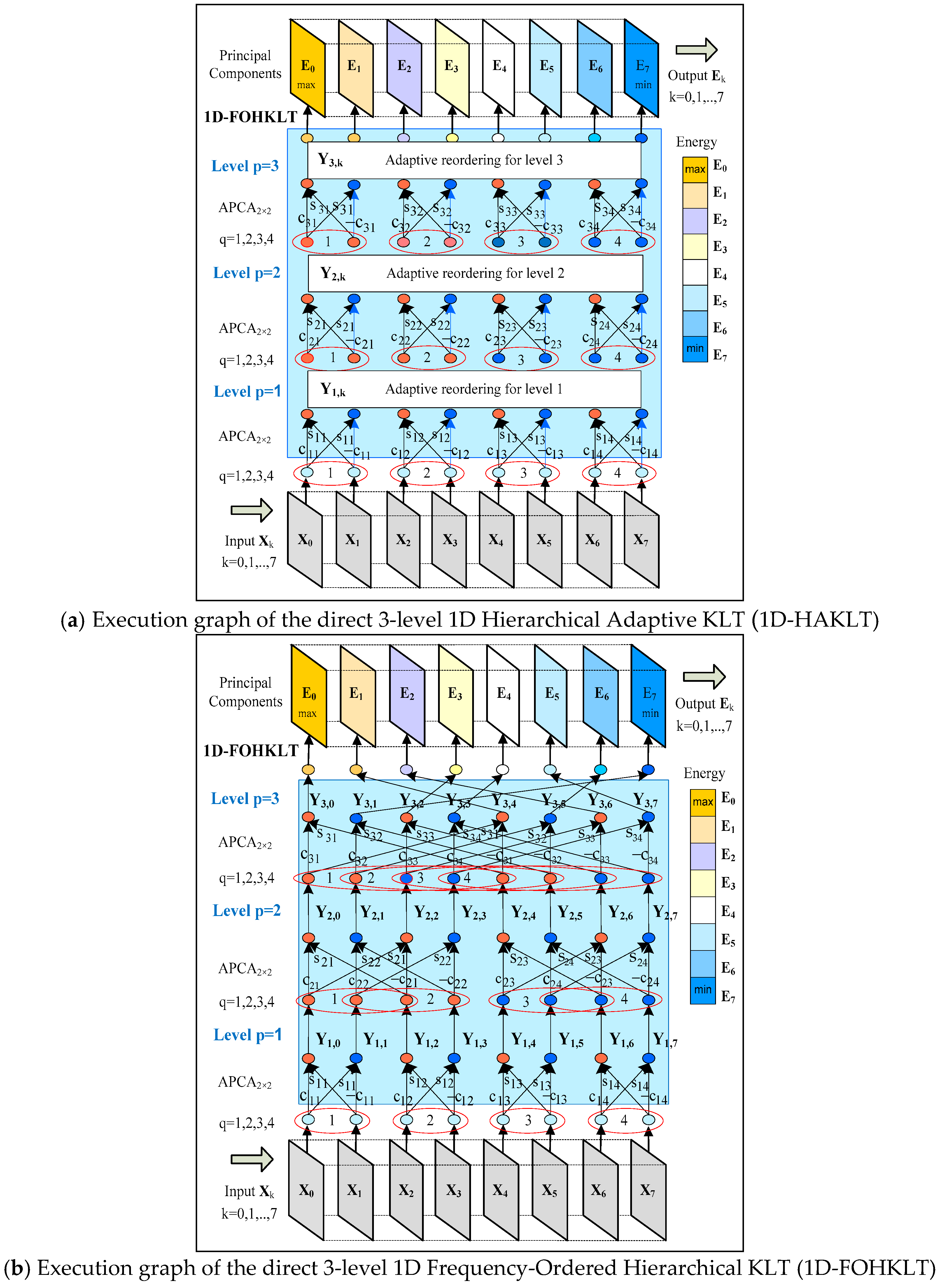
Figure 1. Execution graphs of the direct 3-level transforms 1D-HAKLT and 1D-FOHKLT.
Symmetry 12 01605 g001
Figure 2. Stages of 3D-FOHKLT for the tensor X of size 8 × 8 × 8, based on the 1D-FOKLT.
Symmetry 12 01605 g002
Figure 3. Graphical representation of the relative computational complexity.
Symmetry 12 01605 g003
Table 1. Relative CC of 3D-HAKLT and 3D-FOHKLT compared to H-Tucker and TT.
n2345678
ψ 1 ( n ) 0.230.260.360.570.911.542.68
ψ 2 ( n ) 0.300.350.480.741.212.053.57
ψ 3 ( n ) 0.250.330.500.801.332.284.00
ψ 4 ( n ) 0.330.440.661.061.773.045.33