An Ensemble Machine Learning Technique for Functional Requirement Classification

Abstract

In Requirement Engineering, software requirements are classified into two main categories: Functional Requirement (FR) and Non-Functional Requirement (NFR). FR describes user and system goals. NFR includes all constraints on services and functions. Deeper classification of those two categories facilitates the software development process. There are many techniques for classifying FR; some of them are Machine Learning (ML) techniques, and others are traditional. To date, the classification accuracy has not been satisfactory. In this paper, we introduce a new ensemble ML technique for classifying FR statements to improve their accuracy and availability. This technique combines different ML models and uses enhanced accuracy as a weight in the weighted ensemble voting approach. The five combined models are Naïve Bayes, Support Vector Machine (SVM), Decision Tree, Logistic Regression, and Support Vector Classification (SVC). The technique was implemented, trained, and tested using a collected dataset. The accuracy of classifying FR was 99.45%, and the required time was 0.7 s.

1. Introduction

There are different definitions of requirements in different books and manuals. Considering the definition of the Institute of Electrical and Electronics Engineers (IEEE) standards, a requirement is a capability or condition needed by a user or a system to satisfy an objective [1].

Software requirement classification affects the other activities of Software Development (SD). For example, prioritization—the filtering of relevant requirements—is facilitated by effective classification [2]. Most requirements are classified using two main categories: Functional Requirement (FR) and Non-Functional Requirement (NFR). Sommerville defined FR as services that are expected from a system and their reactions to certain inputs. FR describes both user and system goals. NFR includes all constraints on services and functions [3]. Deeper classification of these two categories can facilitate the SD process [3]. The most common categories of NFR in the reviewed papers can be categorized into four to eleven classes. These classes include maintainability, operability, performance, security, usability, and reliability.

Machine Learning (ML) classifiers have gained importance widely not only in the software engineering field. ML classifiers have recorded the best results in different fields compared with other techniques of classification. In [4] different methods and techniques for forecasting electricity prices have been reviewed, grouped, and discussed in detail. Computational Intelligent tools that are based on ML techniques and Artificial Intelligence (AI) algorithms such as Support Vector Machine (SVM) were described as the best among other statistical methods in modeling the features of pricing electricity. Another area, namely Innovation Capability(IC) where ML showed a significant impact on result improvement and reduction in the number of variables that are required to make decisions is described in [5].Regularized Least Squares, Deep Neural Networks, and Random Forests used in the experiments have been applied on data of the 28 members of European Union(EU). The three used algorithms reduced the complexity of analysis and kept the focus on required features to produce powerful predictions.

NFR statements classification has been a main research concern for a long period of time. Machine Learning (ML) techniques have been adopted for this purpose both widely and successfully. Classification has been tested using many effective algorithms, such as Naïve BayesSVM Decision Tree, and Support Vector Classification (SVC). Furthermore, the datasets for this purpose are available for subsequent researchers. The results of this technique are promising, as it achieved over 90% accuracy in some experiments according to the reviewed published works on the NFR classification objective [2,6,7,8,9,10,11,12,13,14,15,16,17].

On the other hand, FR has not gained as much attention from researchers as NFR, and FR is featured in fewer published papers than NFR [18]. One of the best practices in FR classification is presented in [19], where the FR was classified to six different classes as follows:

• Solution requirements: This type describes the actions that must be carried out by the system or the action that is carried out by the system or the user.
• Enablement requirements: This class determines the capabilities offered to the user by the system. It may determine the subsystem that offers the capability, or it may not determine the subsystem that offers this capability.
• Action Constraint requirements: This class describes the allowable actions for the system or subsystem or the actions that are not allowed. This class also may determine business rules that control some actions in the system.
• Attribute Constraint requirements: This class is related to constraints on attributes or entity attributes.
• Definition requirements: This class is used to define entities.
• Policy requirements: This class is to specify the policies that the system must follow.

The classes described above were shown to satisfy different stakeholders in [19]. Moreover, these classes were used by subsequent researchers successfully in [20].

As manual classification consumes time and requires effort from both analysts and experts, many published papers have tried to successfully transfer the task of classification to automation either via traditional software solutions or using ML models [21]. This paper introduces an enhanced technique for weighted ensemble voting in ML to classify FR into multiple classes. The paper examines a new ensemble approach that uses the accuracy per class from the confusion matrices of the base ML classifiers to create a numerical matrix to store the accuracy per class for each classifier to find the best result and pass it as a weight to the weighted ensemble voting classifier.

The rest of the paper is organized as follows. Section 2 features a review of related works. Section 3 provides the materials and methods. Experimental details are outlined in Section 4. Then, the results are detailed in Section 5, followed by a discussion in Section 6. Finally, the work is concluded in Section 7.

2. Related Work

This section summarizes the previous works on classifying FR using traditional manual techniques or automated techniques and the works that utilized ML techniques to classify FR to various categories.

2.1. Traditional Techniques of Classification

In [19], the authors aimed to analyze software requirements using a tool called a Requirement Analysis Tool (RAT). This tool is intended for use by different stakeholders, such as end users and analysts. FR statements were categorized under different classes: solutions, enablement, action constraints, attribute constraints, definitions, or policy requirements. This method used the Lexical analyzer for tokenization and classification. Then, it used a syntactic analyzer. Although the classification and analysis were conducted using a traditional methodology, the results were promising. This method resulted in a decrease of 30–50% in the required time to review the requirements.

H. Elazhary (2011) adopted the RAT for use in translation between English and Arabic software requirements and developed the Arabic Requirement Analysis Tool (ARAT). Tokenization and classification conducted using a lexical analyzer were then followed by the use of a syntactic analyzer. Many ambiguity issues were resolved by translating software requirements between English and Arabic [20]

A. Ghazarian (2012) categorized FR into different classes: data input, data output, data validation, business logic, data persistence, communication, event trigger, user interface, user interface navigation, user interface logic, event trigger, external call, and external behavior. The Requirements Research Repository (RRR) was used for this study as it was used successfully by two previous experiments for the same purpose. The data used in the testing included 15 software projects with 1236 functional requirements. The results showed the percentage of each class. The highest percentage was observed for the output data class with a percentage of 26.37% [3].

The authors in [22] classified FR as solutions, enablement, action constraints, attribute constraints, definitions, or policy requirements. The authors used Python version 3.6 to implement an ambiguity prevention tool. The methodology used Finite State Machines (FSMs) to classify each requirement according to the syntax. The authors concluded that classification and transformation are not straightforward.

A. Martinez, M. Jenkins, and C. Quesada-Lopez (2019) sought to identify security requirements from FR through several experiments, such as user activation mapped to security templates featuring authorized access, confidentiality during storage, confidentiality during transmission, unique accounts, and logging authentication events. The experiments were applied to 33 graduate students from the University of Costa Rica divided into three groups. Some conducted the activity online, while the others engaged in the activity offline. Participants were given explanations using videos and presentations. The time taken ranged from 20 min to 194 min. The quality was measured using a scale from one to five, on which the results ranged from 2.66 to 4.57 [23].

2.2. ML Techniques of Classification

Software requirement specifications written in the Japanese language were used as a dataset for classification in [18]. FR statements were classified into four categories: requirements for the user interface, requirements for the database, requirements for system functions, and requirements for the external interface. On the other hand, NFR statements were classified according to eight main categories, and each main category was classified to a subcategory according to International Organization for Standardization (ISO) and the International Electrotechnical Commission (IEC)ISO/IEC25030:2007. After using a Convolutional Neural Network (CNN), the FR had the best results, with 0.89 precision, 0.94 recall, and a 0.91 F-score.

FR statements were classified into seven categories in [1] using Grounded Theory (GT). FR statements were classified into seven classes: external communication, business constraints, business workflow, user interactions, user privileges, user interface, and entity modelling requirements. Supervised learning was applied via ML algorithms, including Naïve Bayes, Bayes net, K-Nearest Neighbourhood, and Random Forest. The different numbers of FR statements in eight documents ranged from 208 to 6187. Precision ranged from 0.39 to 0.60, recall ranged from 0.40% to 0.71%, and the F-measure ranged from 0.47 to 0.60.

About 450 FR statements selected from the insurance domain were used to test and classify FR into eleven categories: audit trail, batch processing, localization, communication, payments, print, report, search, third party interactions, and workflow. The Multinomial Naïve Bayes classifier recorded a recall ranging from 28% to 90% and precision ranging from 50% to 100% [24].

Conceptual clustering is used to classify the FR statements of any project based on previous similar projects. A case study on power supplies was used as an example of applying this approach. FR statements have been classified based on safety requirements, electrical specifications, general specifications, power failure detection for the Federal Communication Commission (FCC), and mechanical specifications, regulations, and ripples. This approach offers the opportunity to utilize the historical knowledge of experts on FR patterns [25].

Since the time needed for classification has been generally improved using automation, this time could be improved further by utilizing ML as in previous studies in general software requirement classification. Ensemble modeling in ML has been utilized only rarely for software requirement classification. In addition, as observed in the reviewed papers, classifying FR to further classes is not as much of a concern as classifying NFR. Thus, this research aims to enhance accuracy as a weight in the weighted ensemble voting approach to classify FR into six classes that were used in previous works [19,20,22] successfully implementing traditional automation approaches.

3. Materials and Methods

This section describes the dataset collection process, the dataset itself, and the proposed methodology to be applied to the collected dataset to achieve the desired objectives.

3.1. Data Collection Description

The dataset was prepared by the authors since there was no available dataset with an acceptable number of FR statements to be classified to the selected six classes. To prepare the dataset, the following activities were undertaken:

• Searching for available sets of FR statements or software specification documents that were offered for research purposes. Several folders contained a number of software specification documents available online [26,27,28,29].
• Collecting a reasonable number of FR statements in a spreadsheet with two columns: requirements and class. We used a total of 600 FR statements that include the same number of each desired class to ensure that the dataset is balanced.
• Labeling each FR according to the syntax of each chosen class as solution, enablement, action constraint, attribute constraint, definition, or policy requirements.

The final dataset is 600 sentences; each is an FR statement that belongs to one specific class. These statements are kept in a spreadsheet and represent the first column that is named “Requirement”. The label of each statement is written in the second column that is named “Label”.

3.2. Methodology

The architecture illustrated in Figure 1 consists of several elements:

• Data Pre-processing.
• Classification using ML base classifiers (SVM, Naïve Bayes, SVC, Decision Tree, and Logistic Regression).
• Building a confusion matrix for each base classifier.
• Calculating the accuracy for each base classifier.
• Generating a numerical array.
• Ensemble classifier (the accuracy per class as a weight in weighted ensemble voting).

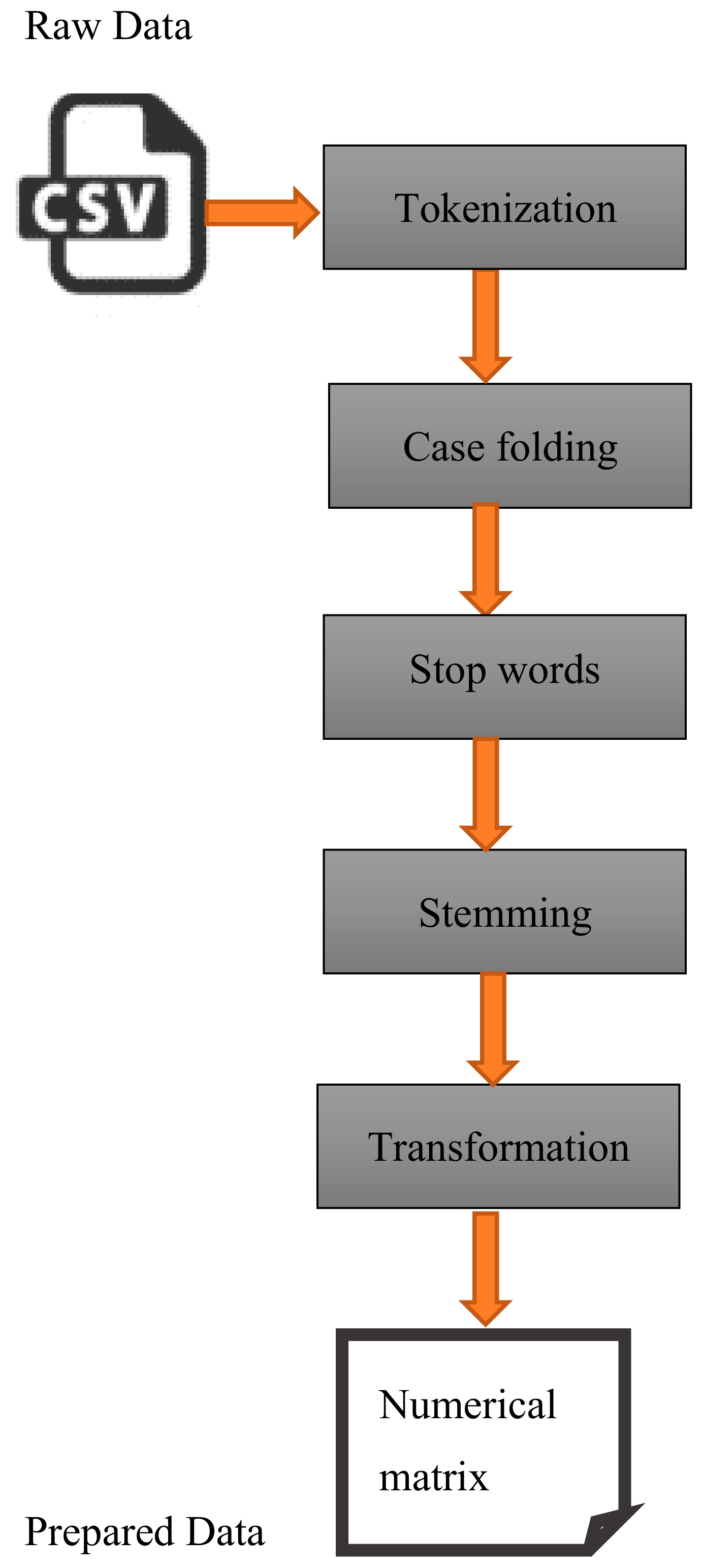
3.2.1. Data Pre-Processing

Pre-Processing involves translating an input requirement into a form that can be processed and passed onto ML or Deep Learning (DL) models using algorithms. ML is related to mathematical intelligence, as the input is determined by its syntactic elements, such as verbs and nouns, or their semantics as a group or domain, which defines variance in meaning. ML, an Artificial Intelligence (AI) application, supports processing tasks using algorithms and classifiers along with training sets for data and testing sets for data [30].

Familiar text preprocessing includes tokenization, case folding, stop word removal, stemming, and transformation. Input data for this research needed to be prepared as a suitable input for the base selected ML classifiers and the ensemble [31]. The steps for pre-processing are mostly the same as those for all base classifiers. As data pre-processing depends on the nature of the research, light pre-processing was used in this study, as shown in Figure 2 below:

• Tokenization is defined as separating the input data into tokens. A token is a group of letters joined with a semantic meaning with no need for further processing. Different tokenization methods can be applied to a text, so it is important to use the same technique for all texts used in an experiment [31]
• Case folding is the process of unifying the cases of the letters in the entire text, but there can be some ambiguity if uppercase letters are used to distinguish different abbreviations [31].
• Stop words are the parts of sentences with negative effects on multiclassification problems. Stop words include prepositions, pronouns, adverbs, and conjunctions [31]
• Stemming refers to extracting the morphological root of a word. Several different techniques are used for this process, including lemmatization, the use of semi-automatic lookup tables, and suffix stripping [31].
• The last step is transformation, which involves using word frequency to provide a score or identification (ID).

The Term Frequency-Inverse Document Frequency (TF-IDF) score for each token is calculated using the following equations:

$$TF-IDF \left(t,d\right)=TF \left(t,d\right) \ast IDF\left(t\right)$$

(1)

$$IDF\left(t\right)=log \left[ n/DF\left(t\right)\right]+1.$$

(2)

Another successful tokenization technique that works similar to TF-IDF is the countvectorizer, which returns a vector with the lengths of all terms in the raw data. This vector is numerical, which is the only difference between TF-IDF and the countvectorizer: the countvectorizer returns an integer count of the number of appearances of each term in the input, while the TF-IDF returns IDs as a result of multiple calculations [32].

3.2.2. ML Classifiers

• Support Vector Machine (SVM) model

SVM is a model that combines the power of conventional theoretical statistical methods and analytical simplicity. Moreover, it works well even on small datasets. Linear SVM classifiers were used in this experiment. The reason we selected linear SVM over non-linear SVM is the smaller amount of time needed for training SVM due to the low complexity in its calculations. Furthermore, classifiers have high dimension data applications and do not require more features to be added [33].

This algorithm is simple and can be described according to the following variables:

$$\mathrm{Training}\mathrm{data}D={\left\{x_i,y_i\right\}}_{\mathrm{i}=1}^N$$

(3)

$$\mathrm{Input}\mathrm{vectors}{x}_i={\left(x_i^{\left(1\right)},\dots ,x_i^{\left(n\right)}\right)}^TϵR^n$$

(4)

$$\mathrm{Target}\mathrm{labels}{\mathit{y}}_{\mathit{i}}ϵ\left\{-1,+1\right\}.$$

(5)

The condition is set as follows:

$${\mathit{y}}_{\mathit{i}}\left[{\mathit{w}}^{\mathit{T}}\varnothing \left({\mathit{x}}_{\mathit{i}}\right)+\mathit{b}\right]\ge 1, \mathit{i}=1,\dots ..,\mathit{N}$$

(6)

where w is the weight vector and b is the bias. The non-linear equation is represented as

$$\mathit{\varphi }\left(\cdot \right):{\mathbb{R}}^{\mathit{n}} \to {\mathbb{R}}^{\mathit{n}\mathit{K}}.$$

(7)

In the above equation, the separating hyperplane that comes between two parallel hyperplanes is

$${\mathit{w}}^{\mathit{T}}\mathit{\varphi }\left(\mathit{x}\right)+\mathit{b}=0$$

(8)

with a margin width of $\frac{2}{{\Vert w\Vert }^2}$.

The decision of the classifier follows the formula of

$$\mathit{s}\mathit{g}\mathit{n}\left({\mathit{w}}^{\mathit{T}} \mathit{\varphi }\left(\mathit{x}\right)+\mathit{b}\right).$$

(9)

The final SVM function is

$$\mathit{sgn}\left({{\displaystyle \sum }}_{\mathit{i}}^{\mathit{N}}{\mathsf{\alpha }}_{\mathit{i} }{\mathit{y}}_{\mathit{i}}\mathit{K}\left(\mathit{x},{\mathit{x}}_{\mathit{i}}\right)+\mathit{b}\right).$$

(10)

• Naïve Bayes Model

The Naïve Bayes model is a machine learning classification model that is known for its independence assumption. This means that the probabilities of one instance are not affected by other attributes. It has been reported that the results of the Naïve Bayes classifier are usually accurate. Moreover, the Naïve Bayes classifier can underperform due to different issues caused by training data noise, variance, and bias [34].

According to the explanations of the algorithm in [35], the features or vectors are presented as $X=\left(X_{1,\dots ,}{X}_n\right)$ from domain $D_i$, where lowercase x represents the value of a vector. The unobserved class C is one of the m values represented as $c\in \left\{0,\dots ,m-1\right\}$ and obtained by g(x), where

$$g:\Omega \to \left\{0,\dots ,m-1\right\}$$

$$\Omega =D_1\times \dots \times D_n.$$

The discriminant function t

The Naïve Bayes discrimination function is

$$\mathit{f}{\mathit{i}}^{\mathit{N}\mathit{B}}\left(\mathit{x}\right)={\displaystyle \prod }_{\mathit{j}=1}^{\mathit{n}}\mathit{P}\left({\mathit{X}}_{\mathit{j}}={\mathit{x}}_{\mathit{j}}|\mathit{C}=\mathit{i}\right)\mathit{P}\left(\mathit{C}=\mathit{i}\right)$$

(11)

• Logistic Regression

The predicted values for the dependent variable are found between 0 and 1 by applying the following regression formula [36]:

$$\mathit{y}=\frac{{\mathit{e}}^{{\mathit{b}}_0+{\mathit{b}}_1·{\mathit{x}}_1+\dots +{\mathit{b}}_{\mathit{n}}·{\mathit{x}}_{\mathit{n}}}}{1+{\mathit{e}}^{{\mathit{b}}_0+{\mathit{b}}_1·{\mathit{x}}_1+\dots +{\mathit{b}}_{\mathit{n}}·{\mathit{x}}_{\mathit{n}}}}$$

(12)

The following formula is an example of transforming the probability $p$ of the dependent variable $y$:

$$\acute{\mathit{p}}={\mathit{log}}_{\mathit{e}}\left(\frac{\mathit{p}}{1-\mathit{p}}\right)$$

(13)

where $\acute{p}$ is any value ranging between $+\infty \mathrm{and}-\infty .$ Values transformed in this way will be used in the ordinary linear regression and the final equation is the following:

$$\acute{\mathit{p}}={\mathit{b}}_0+{\mathit{b}}_1·{\mathit{x}}_1+{\mathit{b}}_2·{\mathit{x}}_2\dots +{\mathit{b}}_{\mathit{n}}·{\mathit{x}}_{\mathit{n}}$$

(14)

• Decision Tree

The Decision tree is used to support decision making problems with hierarchical structures. The first node is called the root node, and the nodes that represent the other features until reaching the structure’s final nodes are called leaf nodes, which represent the target classes/labels. Adjacent nodes are linked by branches. The results of testing link the last node at the current level to a node on the next level. The Decision tree has been described as a strong algorithm as it accepts numerical and ostensible features to guarantee the inclusion of all features. Furthermore, large and small datasets can be managed. The reported weaknesses when using large trees (such as biased decisions) do not apply to this research as our dataset is not very large [37].

Standard deviation measures the error in each node split and the decrease on its Standard Deviation Reduction (SDR) calculated using the following formula [38]:

$$\mathit{S}\mathit{D}\mathit{R}=\frac{\mathit{m}}{\left|\mathit{T}\right|} \times \beta \left(i\right)\times \left[\mathit{s}\mathit{d}\left(\mathit{T}\right)-{\displaystyle \sum }_{\mathit{j}\in \left(\mathit{L},\mathit{R}\right)}\frac{\left|{\mathit{T}}_{\mathit{j}}\right|}{\left|\mathit{T}\right|}\times \mathit{s}\mathit{d}\left({\mathit{T}}_{\mathit{j}}\right)\right]$$

(15)

where T represents the samples that reach the node, m is the number of samples with no missing parameters, $\beta \left(i\right)$ noted as the correction factor, and dividing the specific parameter produces left child node (TL) and right child node (TR) sets [38].

• Support Vector Classification (SVC)

In [39], SVC for binary classification problems was analyzed for use in developing a novel approach called Longitudinal SVC. This new approach was successfully designed to enhance performance. Linear SVC aims to classify and categorize the input data after fitting it into a hyperplane. Then, features need to be passed to the classifier. The hyperplane can be linear or nonlinear according to the data. The kernel is a type of hyperplane, while gamma is a value related to the nonlinear kernel. A gamma increase means more fitting of the training data. However, in some cases, it leads to overfitting. There is a penalty value called c that is used to control the correctness of classifying training points and the smoothness of the decision boundary. Moreover, an increase in c may lead to overfitting. In the case of a nonlinear hyperplane ’poly’, the degree value is needed. This value can be set to ‘1′, which indicates a linear hyperplane. An increase in this value will lead to an increase in training time [40,41]

The following formula is used for the SVC algorithm [42]:

$$f\left(x\right)=\left(w,x\right)+b,w\in R^n,b\in R.$$

(16)

The training data are represented as:

$$\left\{\left(x_1,y_1\right),\dots ,\left(x_1,y_1\right)\right\},\mathrm{x}\in R^n,y\in R.$$

(17)

3.2.3. Building a Confusion Matrix for Each Classifier

A confusion matrix is used to display a summary of each classifier performance. Each row represents the predicted class, and each column represents the actual class. Diagonal elements represent the recall values, and these values divided by the sum are the precision values [43].

3.2.4. Calculating the Accuracy for Each Base Classifier

The accuracy represents correctly classified data in proportion to the total data according to the following formula [44]:

$$\mathit{Accuracy}= \frac{\sum \mathit{True} \mathit{Positive}+ \sum \mathit{True} \mathit{Negative}}{\sum \mathit{Total} \mathit{Population}}$$

(18)

3.2.5. Generating the Numerical Matrix

As enhancing the proposed ensemble classifier depends on the accuracy per class for each classifier, that accuracy needs to be calculated. Thus, the best classifier for each class needs to be determined. This process depends on the confusion matrices for all classifiers. In more detail, this refers to the classifier that manages to make the highest number of correct predictions for each class in the confusion matrix. To determine this classifier, a matrix was created to be filled using the confusion matrices of the base classifiers. The following is an example of how the matrix is filled from the confusion matrices. The classes are given numbers from 0 to 5, and the two classifiers are named A and B (Figure 3):

In the above example (Figure 3), the best classifier for class 0 is classifier B, while the best for class 1 is classifier B. For class 2 and 3, both classifiers are equal. Thus, one of them will be chosen randomly. For class 4, classifier A is best, while for class 5, classifier B is best.

3.2.6. Ensemble Classifier

These classifiers are different to existing ensemble approaches that combine ML classifiers to improve accuracy. The following are some of the most common models:

• Mean Ensemble Voting

In this type, the ensemble works to find the average decisions of all base classifiers according to the following equation adopted from [45]:

$$\widehat{\mathit{y}}=\mathit{Average}\{{\mathit{C}}_1\left(\mathit{x}\right)+{\mathit{C}}_2\left(\mathit{x}\right),\dots ,{\mathit{C}}_{\mathit{m}}\left(\mathit{x}\right)\}.$$

(19)

• Weighted Ensemble Voting

To predict the class label $\widehat{y}$ considering weight $w_j$ related to classifier $C_j$,

$$\widehat{\mathit{y}}=\underset{\mathit{i}}{\mathit{a}\mathit{r}\mathit{g}\mathit{m}\mathit{a}\mathit{x}}{\displaystyle \sum }_{\mathit{j}=1}^m{\mathit{w}}_{\mathit{j}}\mathit{X}\mathit{A}\left({\mathit{C}}_{\mathit{j}}\left(\mathit{x}\right)=\mathit{i}\right)$$

(20)

where $XA$ is the characteristic function, and A is a set of class labels, which are computed using the following formula:

$$\left[{\mathit{C}}_{\mathit{j}}\left(\mathit{x}\right)=\mathit{i}\in \mathit{A}\right]$$

(21)

• Accuracy in Weight Ensemble Voting

This approach works the same as weighted accuracy by replacing the weight with the accuracy of each base classifier. Here, $w_j$ is replaced by the accuracy, which is calculated by

$$\mathrm{Accuracy}=\frac{\sum \mathrm{True} \mathrm{Positive}+ \sum \mathrm{True} \mathrm{Negative}}{\sum \mathrm{Total} \mathrm{Population}}$$

(22)

• Proposed Ensemble voting

The type of ensemble adopted and modified in this study is Accuracy as Weight Ensemble Voting. The weight reflects the accuracy of each classifier, which already exists and is used in classification. Enhancement will determine the accuracy of each classifier for each class and thereby determine the best classification of each input. This model uses confusion matrices and a numerical array to store the values of the accurate predictions from the confusion matrices. In details, the significance of the proposed ensemble approach is a result of using accuracy of each class or label among all base ML classifiers. As the overall accuracy as an absolute measure of performance is misleading, it is not used in the proposed approach classification decisions. Moreover, due to the differences among base classifiers in the mechanism by which they make decisions, it is difficult to find the best classifier for the whole labelling process. Thus, the strength of each base classifier is utilized in the proposed approach. The following is a description of the approach:

Algorithm 1: Calculating weight for base ML classifiers

Input: X: A data stream of sentences inserted from a file.     Y: a label of the sentences     Clf(i): Number of algorithms used [SVM, SCV, Naïve Bayes, Decision Tree, Logistic Regression]. Output: W: An array of weights assigned for each Clf(i) Voting_ Accuracy: Represents the proposed ensemble voting model. // Data preprocessing stage X<Tokenize sentences in X X<Remove spaces and stop words. X<Convector(X) // convert sentences into numbers Y< Convector (Y) // convert labels (classes) into numbers // split data into training and testing portions train_data (x, y), test_data(x,y) < Split (X, Y) For each model in CLF(i):   Clf(i) < fit (train_data (X, Y))   P(y’) < Predict (test data(X))   Result< Compare(p(y’), Y)   Conf(i)< Calculate (Confusion matrix)   Accuracy(i) < Result / Y*100 End // Give a weight for each model // combine the diagonals of all confusion matrices into one matrix Conf_matrix < [[Conf (i:). diagonal]] // find the maximum of each column that will represent the algorithm weight W < max_coloumn (Conf_matrix(i)) V_result< Voting_algorithm (Clf(i), W(i)) Voting_ Accuracy < V_Result / Y*100

4. Experiment Details

4.1. Dataset

In the experiment, the data set is a list of functional software requirements used in previous real-world projects and found online to be used for research purposes. These requirements were selected according to specific criteria, as they should be free of spelling mistakes or typos. Furthermore, the number of requirements that belong to each class should be equal to obtain a balanced dataset. The total of the used FR statements is 600, as suggested in previous research on software requirement classification. Moreover, the small size of the dataset is not considered a problem with ensemble techniques [46]. The overfitting problem that is usually caused by the small size of a dataset was carefully solved over the selection of the parameters of each ML classifier as suggested in [47]. This means that there are 100 FR statements from each class. To the best of our knowledge, this is the first dataset that includes FR statements labeled to six different classes. The data were preprocessed according to the explained methodology in the proposed model section and were then split into training and testing groups, with the largest portion given to training (70%). This percentage was selected according to the proportion of the number of classes being used and the size of the dataset. We sought to ensure that the dataset was balanced from the beginning (i.e., containing the same number of FR statements from each class) and remained balanced after the split, as 70% training involves 70% from each class and 30% testing involves 30% from each class. This percentage was selected to ensure that the classifiers were trained sufficiently on all classes and learned the syntax of each, while leaving enough data to test the accuracy of each classifier and ensure that it performs well. Moreover, to confirm the assumption of the ideal split of data practically, a set of experiments on different data split percentages were conducted.

4.2. Tools and Instruments

4.2.1. Software

Python 3.6 was used for implementing the base classifiers and the ensemble classifier. We used the PyCharm tool, which is user friendly, and its dataset allows for easy uploading. This is true for various dataset file formats, such as comma-separated values (CSV).

Scikit learn was also chosen, as it includes many libraries that can facilitate building ML classifiers and calculating the factors that were used in the evaluations. Ensemble models are supported widely by all types of classifiers.

4.2.2. Hardware

The computer was an ASUS Laptop, with an x64 Inter(R) Core (TM) i7-9750H processor and 17.0 GB of RAM, running a 64-bit Windows Operating System.

5. Results

This section provides the training settings and the results of the testing phase according to the percentage of the dataset split between training and testing (70–30%).

5.1. Training

The parameters of each ML classifier must be specified, as they affect the results dramatically. For the SVM classifier, the parameters that need to be specified are c (cost), kernel, degree, and gamma. C is a regularization parameter since it controls the tradeoff between misclassification and large margins of error. Its value can be 1, 10, 100, or 1000, as a small value leads to constraint ignorance with a large margin of error, and vice-versa. The default value is 1.0. The kernel parameter is used to specify the kernel type, which can be ‘linear’, ‘poly’, ‘rbf’, ‘sigmoid’, ‘precomputed’, or callable. The default is ‘rbf’. The degree is only considered in case of a polynomial, and its default value is three. Gamma is a coefficient of the kernel in case it is ‘poly’, and this value determines the influence of the training example on the decision boundary. The default is ‘scale’, which can also be set to ‘auto’ [48,49]. The Naïve Bayes classifier has different parameters that need to be specified, including alpha, fit_prior, and class_prior. Alpha is the smoothing parameter and can be assigned to zero when there is no smoothing, while the default is 1.0. fit_prior is a Boolean parameter that indicates the learning of prior probabilities, and its default value is true. Class_prior is a parameter that determines whether to adjust the class data according to the priors, and the default value is zero [50]. SVC has more parameters that must be declared, but the main parameters are similar to SVM and set to default if linear SVC is selected. By default, the kernel is set to ‘rbf’, gamma is set to ‘scale’, and c = 1.0 [51]. The decision tree’s first parameter is max_depth, which indicates the depth of the tree, where a deeper result indicates more splits and more gathered information. The range of max_depth is from 1 to 32. min_samples_split is a parameter used to assign the number of samples in each node, which can use one as the minimum or all samples as the maximum. Furthermore, the smallest required number of samples in each leaf can be defined through the min_samples_leaf parameter. max_features is related to the maximum number of features during the split [52]. The Logistic Regression algorithm also has parameters that must be set. The most important parameter is the regulation parameter c, where c = $\frac{1}{\lambda }$, and $\lambda$ controls the tradeoff between the complexity and simplicity of the model. A lower value of $\lambda$ means a more complex model, which indicates an overfit, and vice-versa. On the other hand, a c parameter that produces an opposite result for small values increases the simplicity of the model and is called underfitting, while high values increase complexity and facilitates better adjustments of the data [53].

5.2. Testing

To find the best approach for the proposed enhanced ensemble ML classifier, a number of experiments were conducted. The base ML classifiers and the proposed enhanced ensemble approach were tested under different circumstances.

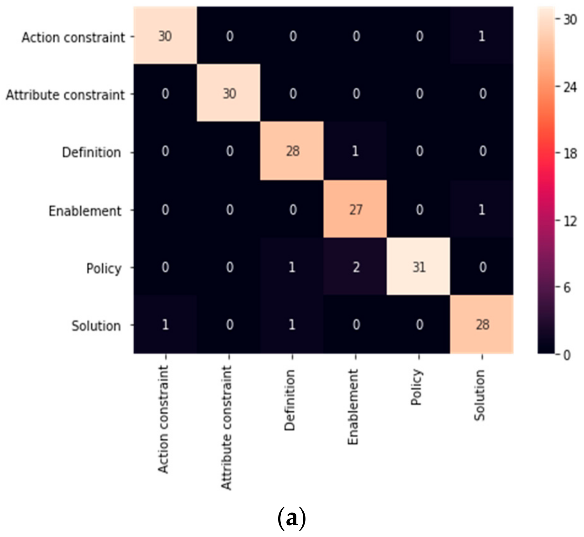
• First, the base ML classifier performance was tested using preprocessing with TF-IDF and Countvectorizer. The results are shown in Figure 4 and Figure 5, which illustrate the confusion matrices for the base classifiers, and

  Table 1. Accuracy and time using TF-IDF and Countvectorizer.

  Classifier	Accuracy (%)		Time (Seconds)
  	TF-IDF	Countvectorizer	TF-IDF	Countvectorizer
  Decision Tree(DT)	73.0	96.0	0.123668	0.017952
  Support Vector Machine (SVM)	79.0	99.0	0.097742	0.104719
  Support Vector Classification (SVC)	75.0	97.0	1.979704	0.621348
  Logistic Regression(LR)	79.0	99.0	0.016955	0.013964
  Naïve Bayes(NB)	70.0	95.0	0.008976	0.007967
  Proposed Ensemble	79.12	99.45	2.175181	0.750992

  , which summarizes the accuracy and required time for each base classifier in the proposed enhanced ensemble approach.
• Second, different data split percentages of training and testing data have been tested (50:50, 40:60, 30:70, 20:80, 10:90) to find the idle split for the ML classifiers. The results are shown in

  Table 2. Accuracy and time using different data split percentages.

  Data Split (Testing: Training) Classifier	50:50		40:60		30:70		20:80		10:90
  	Accuracy (%)	Time (Seconds)	Accuracy (%)	Time (Seconds)	Accuracy (%)	Time (Seconds)	Accuracy (%)	Time (Seconds)	Accuracy (%)	Time (Seconds)
  DT	96.0	0.040	95.0	0.032	96.0	0.018	97.0	0.080	97.0	0.064
  SVM	99.0	0.288	99.0	0.216	99.0	0.105	99.0	0.256	100	0.280
  SVC	97.0	1.280	97.0	1.549	97.0	0.621	97.0	2.175	97.0	2.435
  LR	99.0	0.032	98.0	0.032	99.0	0.014	99.0	0.040	100	0.040
  NB	94.0	0.024	95.0	0.016	95.0	0.008	96.0	0.024	93.0	0.016
  Proposed Ensemble	99.3	1.567	99.1	1.855	99.45	0.751	99.1	2.614	100	2.866

  , which summarizes the accuracy and required time for each base classifier in the proposed enhanced ensemble approach.
• Third, the best three ML classifiers in terms of accuracy are selected to form the proposed ensemble approach, and the results are shown in Figure 6 and

  Table 3. Accuracy and Time using the three most accurate classifiers and the proposed ensemble.

  Classifier	Accuracy (%)	Time (Seconds)
  SVM	99.0	0.084772
  SVC	97.0	0.612361
  Logistic Regression	99.0	0.017953
  Proposed Ensemble	99.45	0.740020

  (accuracy and required time).
• Fourth, the best three base ML classifiers in terms of required time are selected and used to form the proposed ensemble approach. The results are shown in Figure 7 and

  Table 4. Accuracy and time for the three fastest classifiers and proposed ensemble.

  Classifier	Accuracy (%)	Time (Seconds)
  Decision Tree	96.0	0.013962
  Logistic Regression	99.0	0.012965
  Naïve Bayes	95.0	0.006983
  Proposed Ensemble	95.05	0.037898

  .

Both preprocessing techniques, TF-IDF and Countvectorizer, were tested using the five base ML classifiers. The experiments revealed the performance of each preprocessing technique. By comparing the accuracy and time of the confusion matrices, Countvectorizer was shown to outperform TF-IDF in all aspects for all classifiers and the proposed ensemble. Thus, Countvectorizer was selected for preprocessing during the rest of the experiments. The proposed approach achieved 79.8% accuracy using TF-IDF due to the low accuracy of the base ML classifiers, and the required time was 2.17 s. TF-IDF, however, required less than one second (0.7) and achieved 99.45% accuracy.

Different split percentages were tested using the five base ML classifiers. The performance of each classifier was revealed under different split percentages. As the performance attributes include accuracy and time, the ideal split percentage is the one that shows best accuracy and time for the majority of ML classifiers as well as the proposed ensemble approach. From the table below it is clear that in case of splitting the dataset, 30% testing and 70% training are the best percentage splits to be used for the rest of the following experiments. The other data split percentages could show better accuracy for some ML classifiers and the proposed ensemble as well such as 10:90. On the other hand, it increased the time sharply as it doubled in some cases.

We retained only the three most accurate ML base classifiers, SVM, SVC, and Logistic Regression (with accuracies of 99.0%, 97.0%, and 99.0%, respectively), to monitor the accuracy of the proposed ensemble approach, as well as the elapsed time. We noted that the accuracy remains the same when using all five base ML classifiers. In both cases, the accuracy was 99.45%, while the time was enhanced slightly. Next, the three fastest ML base classifiers, Decision Tree, Logistic Regression, and Naïve Bayes (with recorded times of 0.013962 s, 0.012965 s, and 0.006983 s, respectively), were tested to monitor the effects on the accuracy and time of the proposed ensemble approach. Choosing the fastest ML classifiers regardless of accuracy decreased the accuracy of the proposed ensemble approach dramatically to 95.05%. The time improved to 0.037 s. Since time is of secondary concern after accuracy, this approach failed to meet the research objective. The most accurate classifiers required an acceptable time, while the fastest ML classifiers did not record acceptable accuracy compared to the rest of the base ML classifiers. Thus, only the three most accurate classifiers allow the proposed ensemble approach to achieve the objective of the research, which is to enhance accuracy in an acceptable timeframe for classifying FR.

5.3. Comparative Analysis

5.3.1. Experimental Section

This section compares the proposed ensemble approach (using the most accurate ML classifiers after conducting experiments) with existing ensemble approaches.

• Based on time and accuracy

Table 5. Accuracy and time comparison between the proposed ensemble approach and some existing ensemble approaches.

Ensemble	Accuracy (%)	Time (Seconds)
Mean Ensemble Voting	97.80	0.001001
Weighted Ensemble Voting (classifier Importance as weight)	98.35	0.001001
Accuracy as Weight Ensemble	97.25	0.749387
Proposed Ensemble	99.45	0.740020

illustrates the accuracy and the time of some existing ensemble approaches, including the proposed ensemble. Uniquely, the accuracy of the proposed approach reached 99.45%, which was the highest result. However, the time was not the best. Nevertheless, the time required was no longer than the worst time and remained acceptable for automated tools as a response time of classification. The worst ensemble accuracy was about 97% for accuracy as a weight approach, which depends on the overall accuracy of the base classifiers and is a misleading parameter when used alone. In that case, it provides sufficient accuracy to serve as a weight in voting. The mean ensemble provided the same percentage, which is problematic because the ensemble ignores accuracy completely and depends on the average of the base classifiers’ decisions. Considering the importance of the classifiers as weights, the ensemble offered a better accuracy of 98.35%, with the mean ensemble providing the best time of 0.001001 s.

• Based on Receiver Operating Characteristic (ROC) metric

The ROC metric is used to compare the output quality of different classifiers. The Y axis represents the true positive rate while the false positive rate is represented on the X axis. The larger area under the curve (AUC) represents better quality [54]. According to Figure 8, among the existing ensemble approaches the proposed ensemble approach has the best ROC curve and the largest AUC (0.96).

5.3.2. Theoretical Section

Table 6. Comparison of the proposed approach with the state-of-the-art methods in Functional Requirement (FR) classification.

	Reference# (Year)	Classes	Methodology	Dataset	Results
Traditional Classification Technique	[19] (2009)	Solution Enablement Action Constraint Attribute Constraint Definition Policy	Lexical Analyzer Syntactic Analyzer	Not specified	30–50% reduction in time needed to review requirements
	[20] (2011)	Solution Enablement Action Constraint Attribute Constraint Definition Policy	Lexical Analyzer Syntactic Analyzer	Not specified	Many ambiguities were resolved while translating software requirements between English and Arabic.
	[3] (2012)	Data input Data output Data validation Business logic Data Persistence Communication Event Trigger User Interface User Interface Navigation User Interface Logic Event Trigger External Call External Behavior	Use of frequency distributions as a means to characterize the phenomena of interest in a particular domain.	15 software projects with 1236 FR statements.	The highest percentage was for the output data class with a percentage of 26.37%
	[22] (2018)	Solution Enablement Action Constraint Attribute Constraint Definition Policy	Tokenization Reading Classifying Using Finite State Machines (FSMs) Python 3.6 to implement the ambiguity prevention tool.	40 requirements	Classification and transformation processes are not straightforward
	[23] (2019)	Security Requirement Templates such as Authorized access Confidentiality during storage Confidentiality during transmission Unique accounts Logging authentication Events	3 groups: online and offline activity Training: 4-page reference materials, 10 min video on security objectives and requirements, and a 15 min explanatory presentation in Spanish Domain: healthcare and banking	Not specified	Time: ranged from 20 min to 193 min Quality: from 2.66 to 4.57 (scale from 1 to 5)
ML Classification Technique	[18] (2018)	Requirements for user interfaces Requirements for databases Requirements for system functions Requirements for external interfaces	Convolutional Neural Networks (CNN)	Software Requirement Specification (SRS) in the Japanese language including 13 systems 11,538 FR-QR- Non-Requirements (Unbalanced data)	Precision: 0.89 Recall: 0.94 F-score: 0.91
	[1] (2015)	External Communication Business Constraints Business Workflow User Interactions User Privileges User Interfaces Entity Modelling	Naïve Bayes Bayes net K-Nearest Neighborhood Random Forest	Eight documents with different numbers of FR statements ranging from 208 to 6187.	Precision: from 0.39 to 0.60 Recall: from 0.40 to 0.71 F-measure: from 0.47 to 0.60
	[24] (2015)	Audit trail Batch processing localization Communication Payments Printing Reporting Searching Third party interactions Workflow	Multinomial Naïve Bayes	450 FR statements selected from the insurance domain	Recall ranged from 28% to 90% Precision ranged from 50% to 100%.
	[25] (97)	Safety requirements Electrical specifications General specifications Power failure detection Federal Communications Commission (FCC) Mechanical specification regulations Ripple	Conceptual Clustering	Case study of power supply product designs	This approach opens the opportunity to utilize historical knowledge through experts on FR patterns.
	Proposed Approach	Solution Enablement Action Constraints Attribute Constraints Definitions Policy	Naïve Bayes, Support Vector Machine (SVM), Decision Tree, Logistic Regression, and Support Vector Classification (SVC).	600 FR statements, as there were 100 FR statements from each class.	Accuracy: 99.45% Time: 0.7 s

theoretically compares the proposed ensemble approach with existing state-of-the-art methods that classify FR into different classes. These works have been classified according to the above sections as traditional approaches or ML approaches.

6. Discussion

The main difficulty in building the necessary datasets was collecting a sufficient number of valid FR statements that could fit the syntax of the six different classes of classification and then labelling them correctly in the spreadsheet. This process consumed a large amount of the experimental process time. The second difficulty related to the dataset was the preprocessing, as most of previous studies used TF-IDF. However, in this work, TF-IDF showed poor performance for all ML classifiers, which affected the performance of the proposed ensemble approach. Thus, the Countvectorizer was adopted. This method improved the efficiency of all ML classifiers and consequentially affected the performance of the proposed ensemble approach, as shown in Figure 5 and Table 1.

Overall, the ML classifiers performed well, and their accuracy values were above 90%. The best performance was recorded for SVM and Logistic Regression, with 99%, and the worst was 97% for the SVC classifier. In this case, the ensemble was able to avoid most of the errors made by the ML classifiers, and its accuracy was 99.45%, which is higher than any values for prior ML classifiers. These results were recorded in the experiments that used the three most accurate ML classifiers and the experiment that used the five ML classifiers, as the proposed ensemble approach selects the best performance among all classifiers. Thus, ML classifiers with poor performance did not affect performance.

In detail, the applied ML classifiers produced different areas of errors, as different ML classifiers misclassified different classes, as shown in the confusion matrices in Figure 8. Thus, because different ML classifiers use different methodologies in classification, they produce different areas of errors.

The time consumed by the proposed ensemble approach was improved by using the fastest ML classifiers. However, the accuracy decreased to 95.05%, as the ML classifiers performed poorly compared to the other excluded ML classifiers. On the other hand, the time consumed by the proposed ensemble approach using the five ML classifiers was slightly longer than the time when using the three most accurate classifiers (the difference was nearly 0.01 s).

Comparing the proposed ensemble approach with existing state-of-art methods showed that the proposed ensemble approach outperformed the others in accuracy. Although our method did not offer the best time, it still produced an acceptable time that did not exceed one second (0.7 s).

The previous experiments offer only one way of proving this concept, a process that will continue in future studies. For example, a Deep Learning ensemble approach should be discovered and tested. Different approaches for classification could also be tested using this concept. After proving the validity of this concept, future studies can integrate large-scale datasets with the proposed ensemble approach.

7. Conclusions

This research introduced an ensemble model that enhances the weighted voting ensemble by using the accuracy per class for each base ensemble to determine the best classification for FR in six classes to enhance accuracy and availability. This model was developed using the ML classifiers of SVM, SVC, Naïve Bayes, Decision Tree, and Logistic Regression. Using the five classifiers gave the same accuracy (99.45%) with the proposed ensemble when using only the ML base classifiers with the highest accuracies (SVM, SVC, and Logistic Regression); only the time decreased, which indicates improvement when using a smaller number of classifiers. The proposed approach was compared to other existing ensemble approaches on the created dataset, and our technique offered the best accuracy among them, with 99.45%. The required time was not the best in our model but was still acceptable as a classification time for automated requirement analysis tools, as it did not reach one second (0.7 s).

References

1. Sharma, R.; Biswas, K.K. Functional requirements categorization: Grounded theory approach. In Proceedings of the 2015 International Conference on Evaluation of Novel Approaches to Software Engineering (ENASE), Barcelona, Spain, 29–30 April 2015; pp. 301–307. [Google Scholar] [CrossRef]
2. Abad, Z.S.H.; Karras, O.; Ghazi, P.; Glinz, M.; Ruhe, G.; Schneider, K. What Works Better? A Study of Classifying Requirements. In Proceedings of the 2017 IEEE 25th International Requirements Engineering Conference (RE), Lisbon, Portugal, 4–8 September 2017; pp. 496–501. [Google Scholar]
3. Ghazarian, A. Characterization of functional software requirements space: The law of requirements taxonomic growth. In Proceedings of the 2012 20th IEEE International Requirements Engineering Conference (RE), Chicago, IL, USA, 24–28 September 2012; pp. 241–250. [Google Scholar] [CrossRef]
4. Weron, R. Electricity price forecasting: A review of the state-of-the-art with a look into the future. Int. J. Forecast. 2014, 30, 1030–1081. [Google Scholar] [CrossRef] [Green Version]
5. Ponta, L.; Puliga, G.; Oneto, L.; Manzini, R. Identifying the determinants of Innovation Capability With Machine Learning and Patents. IEEE Trans. Eng. Manag. 2020, 1–11. [Google Scholar] [CrossRef]
6. Casamayor, A.; Godoy, D.; Campo, M. Identification of non-functional requirements in textual specifications: A semi-supervised learning approach. Inf. Softw. Technol. 2010, 52, 436–445. [Google Scholar]
7. Slankas, J.; Williams, L. Automated extraction of non-functional requirements in available documentation. In Proceedings of the 1st International Workshop on Natural Language Analysis in Software Engineering (NaturaLiSE), San Francisco, CA, USA, 25 May 2013; pp. 9–16. [Google Scholar]
8. Kurtanovic, Z.; Maalej, W. Automatically Classifying Functional and Non-functional Requirements Using Supervised Machine Learning. In Proceedings of the 2017 IEEE 25th International Requirements Engineering Conference (RE), Lisbon, Portugal, 4–8 September 2017; pp. 490–495. [Google Scholar]
9. Mahmoud, M. Software Requirements Classification using Natural Language Processing and SVD. Int. J. Comput. Appl. 2017, 164, 7–12. [Google Scholar] [CrossRef]
10. Singh, P.; Singh, D.; Sharma, A. Rule-based system for automated classification of non-functional requirements from requirement specifications. In Proceedings of the 2016 International Conference on Advances in Computing, Communications and Informatics, ICACCI 2016, Jaipur, India, 21–24 September 2016; pp. 620–626. [Google Scholar]
11. Navarro-Almanza, R.; Juurez-Ramirez, R.; Licea, G. Towards Supporting Software Engineering Using Deep Learning: A Case of Software Requirements Classification. In Proceedings of the 5th International Conference on Software Engineering Research and Innovation (CONISOFT’17), Yucatán, Mexico, 25–27 October 2017; pp. 116–120. [Google Scholar]
12. Taj, S.; Arain, Q.; Memon, I.; Zubedi, A. To apply data mining for classification of crowd sourced software requirements. In Proceedings of the ACM International Conference Proceedings Series, Phoenix, AZ, USA, 26–28 June 2019; pp. 42–46. [Google Scholar]
13. Dalpiaz, F.; Dell’Anna, D.; Aydemir, F.B.; Çevikol, S. Requirements classification with interpretable machine learning and dependency parsing. In Proceedings of the International Conference on Industrial Engineering and Applications (ICIEA), Jeju Island, Korea, 23–27 September 2019; pp. 142–152. [Google Scholar]
14. Baker, C.; Deng, L.; Chakraborty, S.; Dehlinger, J. Automatic multi-class non-functional software requirements classification using neural networks. In Proceedings of the IEEE 43rd Annual Computer Software and Applications Conference (COMPSAC), Milwaukee, WI, USA, USA, 15–19 July 2019; Volume 2, pp. 610–615. [Google Scholar]
15. Halim, F.; Siahaan, D. Detecting Non-Atomic Requirements in Software Requirements Specifications Using Classification Methods. In Proceedings of the 1st International Conference on Cybernetics and Intelligent System (ICORIS), Denpasar, Indonesia, 22–23 August 2019; pp. 269–273. [Google Scholar]
16. Parra, E.; Dimou, C.; Llorens, J.; Moreno, V.; Fraga, A. A methodology for the classification of quality of requirements using machine learning techniques. Inf. Softw. Technol. 2015, 67, 180–195. [Google Scholar] [CrossRef]
17. Knauss, E.; Houmb, S.; Schneider, K.; Islam, S.; Jürjens, J. Supporting Requirements Engineers in Recognising Security Issues. Lect. Notes Comput. Sci. 2011, 6606 LNCS, 4–18. [Google Scholar]
18. Tamai, T.; Anzai, T. Quality requirements analysis with machine learning. In Proceedings of the 13th International Conference Evaluation Novel Approaches to Software Engineering (ENASE 2018), Funchal, Madeira, Portugal, 23–24 March 2018; pp. 241–248. [Google Scholar] [CrossRef]
19. Jain, P.; Verma, K.; Kass, A.; Vasquez, R.G. Automated review of natural language requirements documents: Generating useful warnings with user-extensible glossaries driving a simple state machine. In Proceedings of the 2nd India Software Engineering Conference, Pune, India, 23–26 February 2009; pp. 37–45. [Google Scholar] [CrossRef]
20. Alomari, R.; Elazhary, H. Implementation of a formal software requirements ambiguity prevention tool. Int. J. Adv. Comput. Sci. Appl. 2018, 9, 424–432. [Google Scholar] [CrossRef]
21. Elazhary, H. Translation of Software Requirements. Int. J. Sci. Eng. Res. 2011, 2, 1–7. [Google Scholar]
22. Maw, M.; Balakrishman, V.; Rana, O.; Ravana, S. Trends and Patterns of Text Classification Techniques: A Systematic Mapping Study. Malays. J. Comput. Sci. 2020, 33, 102–117. [Google Scholar] [CrossRef]
23. Martinez, A.; Jenkins, M.; Quesada-Lopez, C. Identifying implied security requirements from functional requirements. In Proceedings of the 2019 14th Iberian Conference on Information Systems and Technologies (CISTI), Coimbra, Portugal, 19–22 June 2019; pp. 1–7. [Google Scholar] [CrossRef]
24. Anish, P.R.; Balasubramaniam, B.; Cleland-Huang, J.; Wieringa, R.; Daneva, M.; Ghaisas, S. Identifying Architecturally Significant Functional Requirements. In Proceedings of the 2015 IEEE/ACM 5th International Workshop on the Twin Peaks of Requirements and Architecture, Florence, Italy, 17 May 2015; pp. 3–8. [Google Scholar] [CrossRef]
25. Tseng, M.M.; Jiao, J. A variant approach to product definition by recognizing functional requirement patterns. J. Eng. Des. 1997, 8, 329–340. [Google Scholar] [CrossRef]
26. Formal Methods & Tools GroupNatural Language Requirements Dataset. Available online: http://fmt.isti.cnr.it/nlreqdataset/ (accessed on 20 April 2019).
27. INSPIRE Helpdesk “MIWP 2014–2016” MIWP-16: Monitoring. Available online: https://ies-svn.jrc.ec.europa.eu/documents/33 (accessed on 20 April 2019).
28. What Is a Functional Requirement? Specification, Types, EXAMPLES. Available online: https://www.guru99.com/functional-requirement-specification-example.html (accessed on 20 April 2019).
29. Week 3: Requirement Analysis & Specification-ppt Video Online Download. Available online: https://slideplayer.com/slide/8979379/ (accessed on 20 April 2019).
30. Keezhatta, M. Understanding EFL Linguistic Models through Relationship between Natural Language Processing and Artificial Intelligence Applications. Arab World Engl. J. 2019, 10, 251–262. [Google Scholar] [CrossRef]
31. Petrović, D.; Stanković, M. The Influence of Text Preprocessing Methods and Tools on Calculating Text Similarity. Ser. Math. Inform. 2019, 34, 973–994. [Google Scholar]
32. Brownlee, J. How to Prepare Text Data for Machine Learning with Scikit-Learn. Available online: https://machinelearningmastery.com/prepare-text-data-machine-learning-scikit-learn/ (accessed on 20 June 2020).
33. Chauhan, V.K.; Dahiya, K.; Sharma, A. Problem formulations and solvers in linear SVM: A review. Artif. Intell. Rev. 2019, 52, 803–855. [Google Scholar] [CrossRef]
34. Mukherjee, S.; Sharma, N. Intrusion Detection using Naive Bayes Classifier with Feature Reduction. Procedia Technol. 2012, 4, 119–128. [Google Scholar] [CrossRef] [Green Version]
35. Lee, E.P.F.; Lee, E.P.F.; Lozeille, J.; Soldán, P.; Daire, S.E.; Dyke, J.M.; Wright, T.G. An ab initio study of RbO, CsO and FrO (X2∑+; A2∏) and their cations (X3∑-; A3∏). Phys. Chem. Chem. Phys. 2001, 3, 4863–4869. [Google Scholar] [CrossRef]
36. Navlani, A. Understanding Logistic Regression in Python. Available online: https://www.datacamp.com/community/tutorials/understanding-logistic-regression-python (accessed on 15 June 2020).
37. Arivoli, P.V. Empirical Evaluation of Machine Learning Algorithms for Automatic Document Classification. Int. J. Adv. Res. Comput. Sci. 2017, 8, 299–302. [Google Scholar] [CrossRef]
38. Pham, B.; Jaafari, A.; Avand, M.; Al-Ansari, N.; Du, T.; Yen, H.; Phong, T.; Nguyen, D.; Le, H.; Gholam, D.; et al. Performance Evaluation of Machine Learning Methods for Forest Fire Modeling and Prediction. Symmetry (Basel) 2020, 12, 1022. [Google Scholar] [CrossRef]
39. Steinhaeuser, K.; Chawla, N.V.; Ganguly, A.R. Improving Inference of Gaussian Mixtures using Auxiliary Variables. Stat. Anal. Data Min. 2015, 8, 497–511. [Google Scholar] [CrossRef]
40. Mohtadi, F. In Depth: Parameter Tuning for SVC. Available online: https://medium.com/all-things-ai/in-depth-parameter-tuning-for-svc-758215394769 (accessed on 20 June 2020).
41. Fenner, M. Machine Learning with Python for Everyone Addison-Wesley Data & Analytics Series; Addison-Wesley Professional: Boston, MA, USA, 2019; ISBN1 0134845641. ISBN2 9780134845647. [Google Scholar]
42. Qu, Y.; Qian, X.; Song, H.; Xing, Y.; Li, Z.; Tan, J. Soil moisture investigation utilizing machine learning approach based experimental data and Landsat5-TM images: A case study in the Mega City Beijing. Water (Switz.) 2018, 10, 423. [Google Scholar] [CrossRef] [Green Version]
43. Rhys, H.I. Machine Learning with R, the Tidyverse, and mlr; Manning Publications: New York, NY, USA, 2020; p. 311. [Google Scholar]
44. Hamed, T.; Dara, R.; Kremer, S.C. Intrusion Detection in Contemporary Environments. Comput. Inf. Secur. Handb. 2017, 109–130. [Google Scholar] [CrossRef]
45. Raschka, S. EnsembleVoteClassifier-mlxtend. Available online: http://rasbt.github.io/mlxtend/user_guide/classifier/EnsembleVoteClassifier/ (accessed on 10 July 2020).
46. Maheswari, J. Breaking the Curse of Small Datasets in Machine Learning: Part 1. Available online: https://towardsdatascience.com/breaking-the-curse-of-small-datasets-in-machine-learning-part-1-36f28b0c044d (accessed on 15 September 2020).
47. Alencar, R. Dealing with Very Small Datasets. Available online: https://www.kaggle.com/rafjaa/dealing-with-very-small-datasets (accessed on 10 June 2020).
48. Pedregosa, F.; Varoquaux, G.; Gramfort, A.; Michel, V.; Thirion, B.; Grisel, O.; Blondel, M.; Prettenhofer, P.; Weiss, R.; Dubourg, V.; et al. Scikit-learn Machine Learning in Python. JMLR 2011, 12, 2825–2830. [Google Scholar]
49. Pupale, R. Support Vector Machines(SVM)—An Overview. Available online: https://towardsdatascience.com/https-medium-com-pupalerushikesh-svm-f4b42800e989 (accessed on 18 September 2020).
50. Scikit-learn Sklearn.Naive_Bayes.Multinomialnb—Scikit-Learn 0.23.2 Documentation. Available online: https://scikit-learn.org/stable/modules/generated/sklearn.naive_bayes.MultinomialNB.html (accessed on 18 September 2020).
51. Scikit-learn.org sklearn.svm.LinearSVC—Scikit-Learn 0.23.2 Documentation. Available online: https://scikit-learn.org/stable/modules/generated/sklearn.svm.LinearSVC.html (accessed on 18 September 2020).
52. Fraj, M. Ben InDepth: Parameter Tuning for Decision Tree. Available online: https://medium.com/@mohtedibf/indepth-parameter-tuning-for-decision-tree-6753118a03c3 (accessed on 18 September 2020).
53. Kaggle Tuning Parameters for Logistic Regression. Available online: https://www.kaggle.com/joparga3/2-tuning-parameters-for-logistic-regression (accessed on 19 September 2020).
54. Scikit-Learn Receiver Operating Characteristic (ROC). Available online: https://scikit-learn.org/stable/auto_examples/model_selection/plot_roc.html (accessed on 18 September 2020).
Figure 1. Architecture of the Ensemble Machine Learning Technique.
Symmetry 12 01601 g001
Figure 2. Data Preprocessing phase.
Symmetry 12 01601 g002
Figure 3. Example of finding accuracy per class.
Symmetry 12 01601 g003
Figure 4. Confusion matrices using Term Frequency–Inverse Document Frequency (TF-IDF: (a) Decision Tree, (b) Support Vector Machine (SVM), (c) Support Vector Classification (SVC), (d) Logistic Regression, (e) Naïve Bayes.
Symmetry 12 01601 g004
Figure 5. Confusion matrices using Countvectorizer: (a) Decision Tree, (b) SVM, (c) SVC, (d) Logistic Regression, (e) Naïve Bayes.
Symmetry 12 01601 g005
Figure 6. Confusion matrices for the three most accurate classifiers: (a) SVM, (b) SVC, and (c) Logistic Regression.
Symmetry 12 01601 g006aSymmetry 12 01601 g006b
Figure 7. Confusion matrices for the three fastest classifiers: (a) Decision Tree, (b) logistic Regression, and (c) Naïve Bayes.
Symmetry 12 01601 g007aSymmetry 12 01601 g007b
Figure 8. ROC comparison among ensemble approaches.
Symmetry 12 01601 g008