Author Contributions
V.P. conducted data curation, investigation, data processing, formal analysis and original draft preparation. W.C. conducted formal analysis, validation, review and editing. T.T. provided funding acquisition, conceptualization, resources, formal analysis, review and editing. A.G. conducted provided funding acquisition, review, and editing. All authors have read and agreed to the published version of the manuscript.
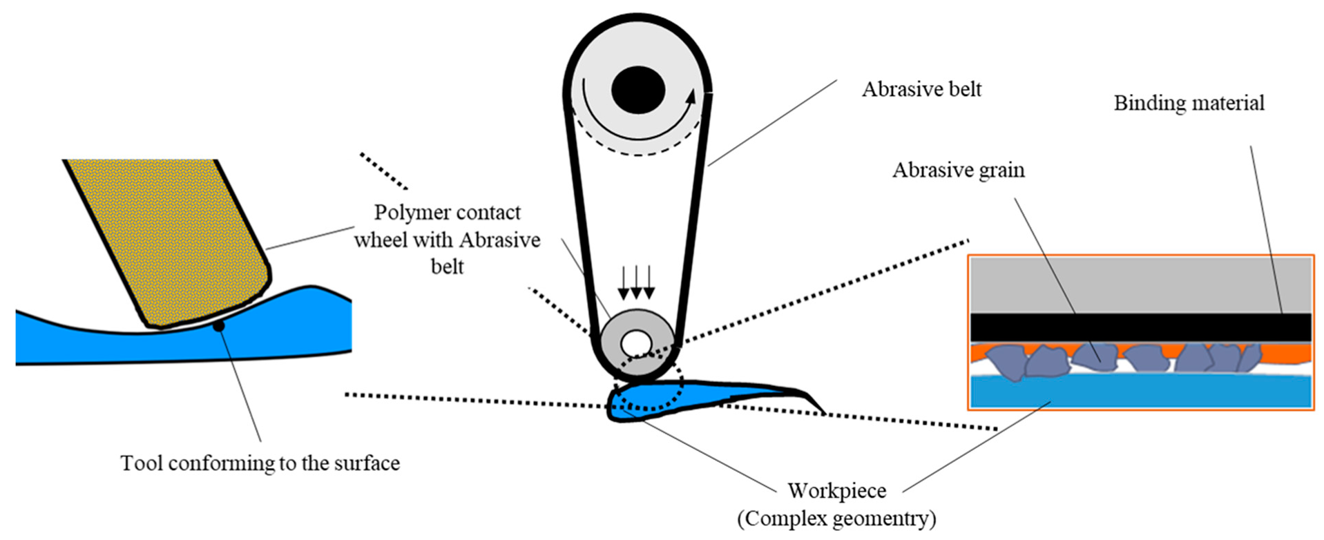
Figure 1.
Principle of the belt grinding process.
Figure 1.
Principle of the belt grinding process.
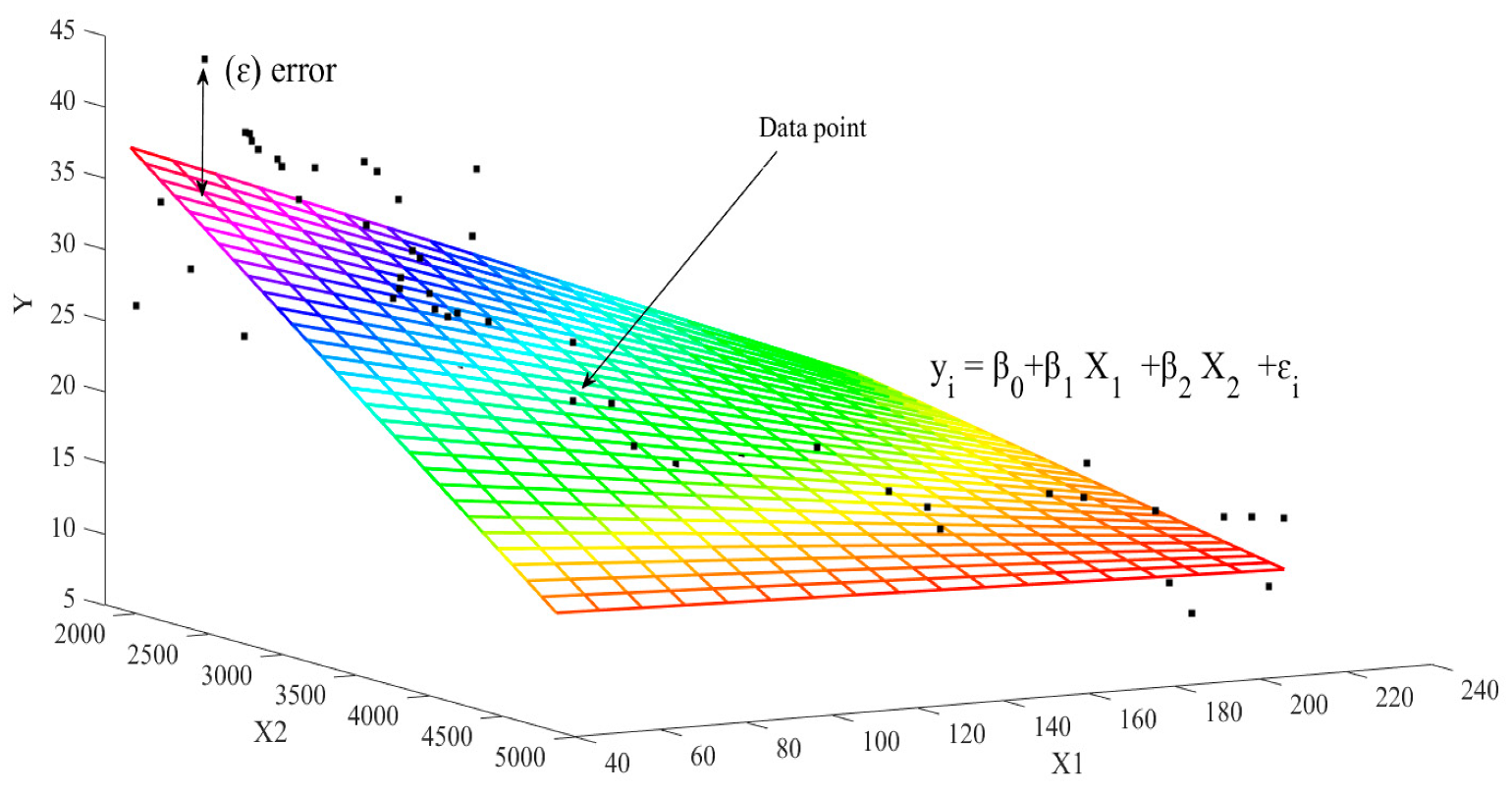
Figure 2.
Surface that corresponds to the simplest multiple regression models.
Figure 2.
Surface that corresponds to the simplest multiple regression models.
Figure 3.
The mathematical model of a neuron.
Figure 3.
The mathematical model of a neuron.
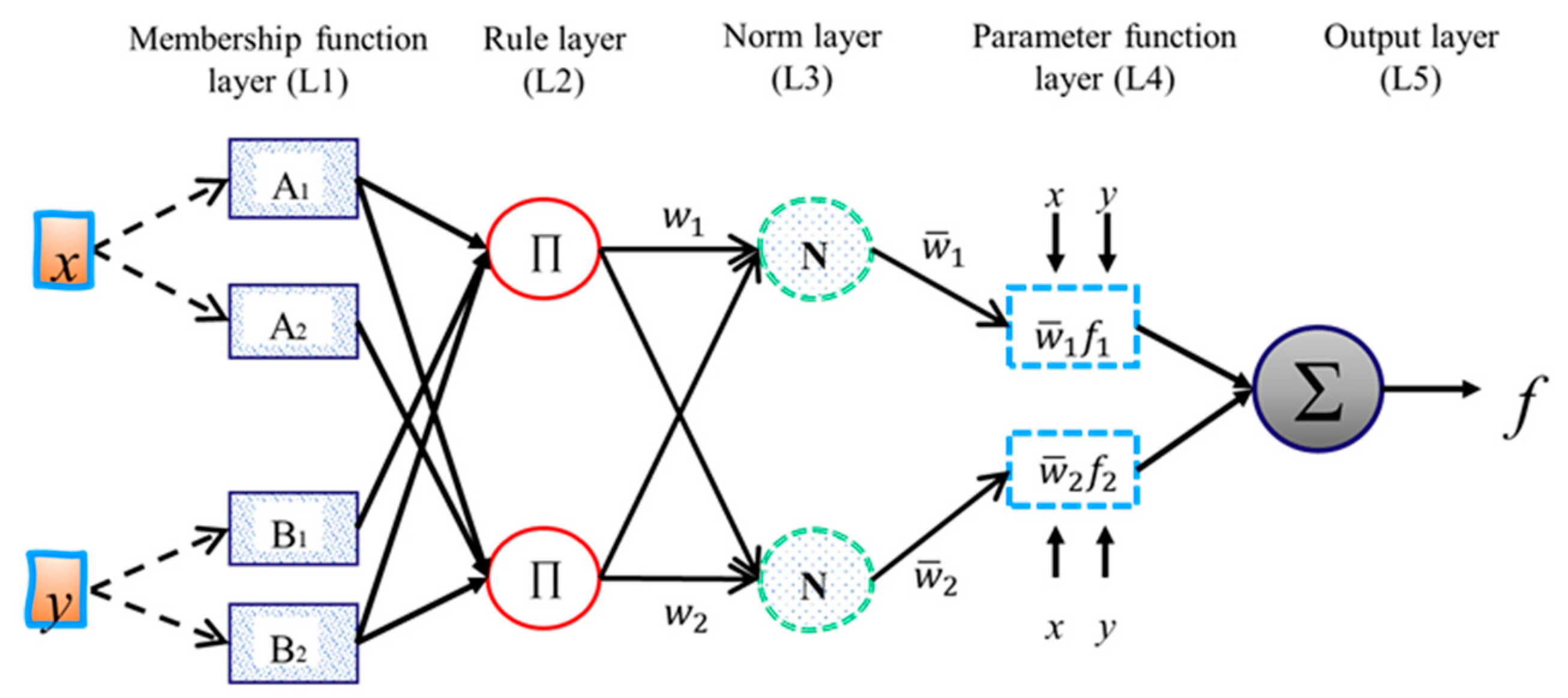
Figure 4.
Adaptive neuro-fuzzy inference system structure.
Figure 4.
Adaptive neuro-fuzzy inference system structure.
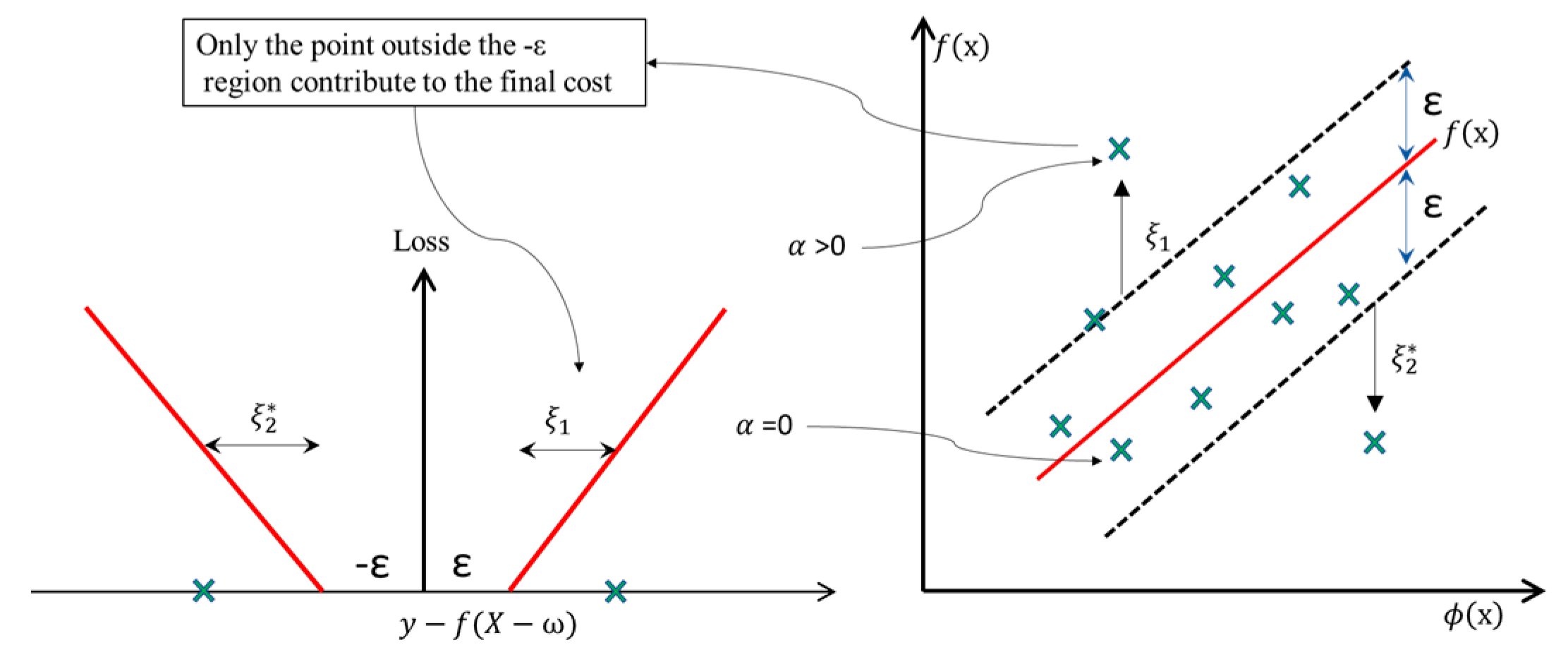
Figure 5.
The regression line of support vector regression (SVR) is shown with the loss function and slack variables.
Figure 5.
The regression line of support vector regression (SVR) is shown with the loss function and slack variables.
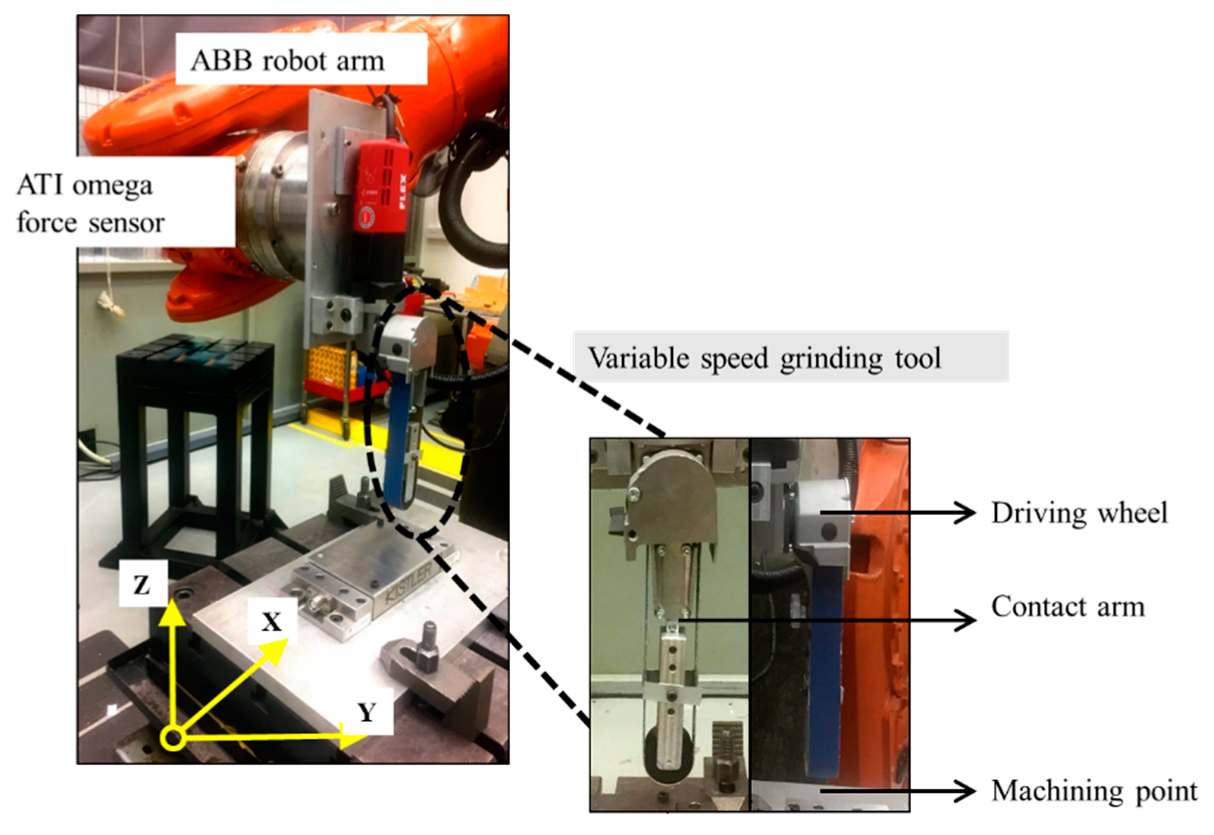
Figure 6.
Compliant abrasive belt grinding experimental setup [
12].
Figure 6.
Compliant abrasive belt grinding experimental setup [
12].
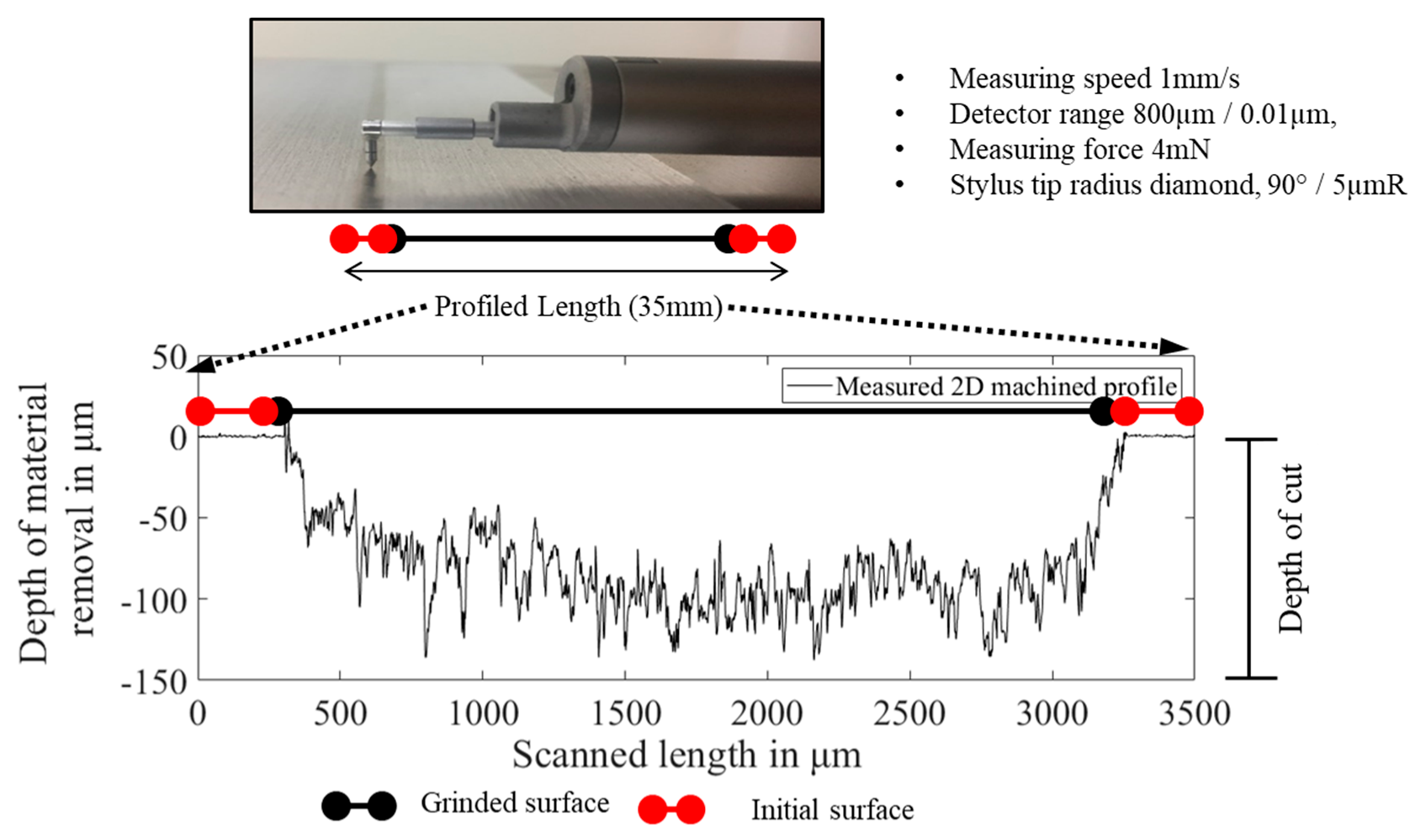
Figure 7.
Mitutoyo contact profilometer used to measure the depth of cut across the grinded path.
Figure 7.
Mitutoyo contact profilometer used to measure the depth of cut across the grinded path.
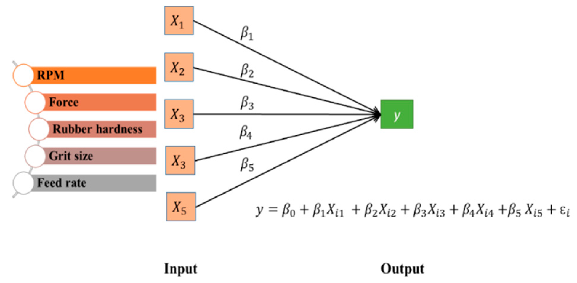
Figure 8.
Schematic illustration of the multilinear regression model for prediction of the material removal.
Figure 8.
Schematic illustration of the multilinear regression model for prediction of the material removal.
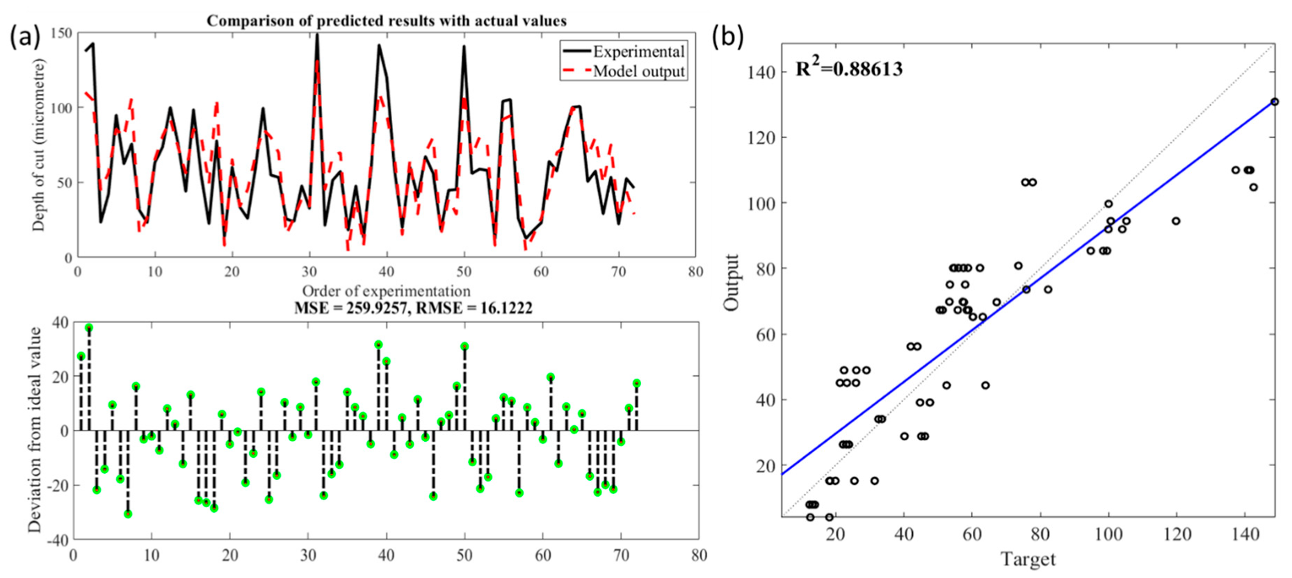
Figure 9.
(a). Comparison of the observed and predicted depth of cut using multilinear regression; (b). Statistical analysis fit of the multilinear regression model.
Figure 9.
(a). Comparison of the observed and predicted depth of cut using multilinear regression; (b). Statistical analysis fit of the multilinear regression model.
Figure 10.
(a). Comparison of observed and predicted depth of cut using stepwise regression; (b) Statistical analysis fit of the stepwise regression model.
Figure 10.
(a). Comparison of observed and predicted depth of cut using stepwise regression; (b) Statistical analysis fit of the stepwise regression model.
Figure 11.
Residual plot observed between the multilinear regression model and stepwise multilinear regression model.
Figure 11.
Residual plot observed between the multilinear regression model and stepwise multilinear regression model.
Figure 12.
Schematic illustration of an artificial neural network (ANN) model for prediction of the material removal.
Figure 12.
Schematic illustration of an artificial neural network (ANN) model for prediction of the material removal.
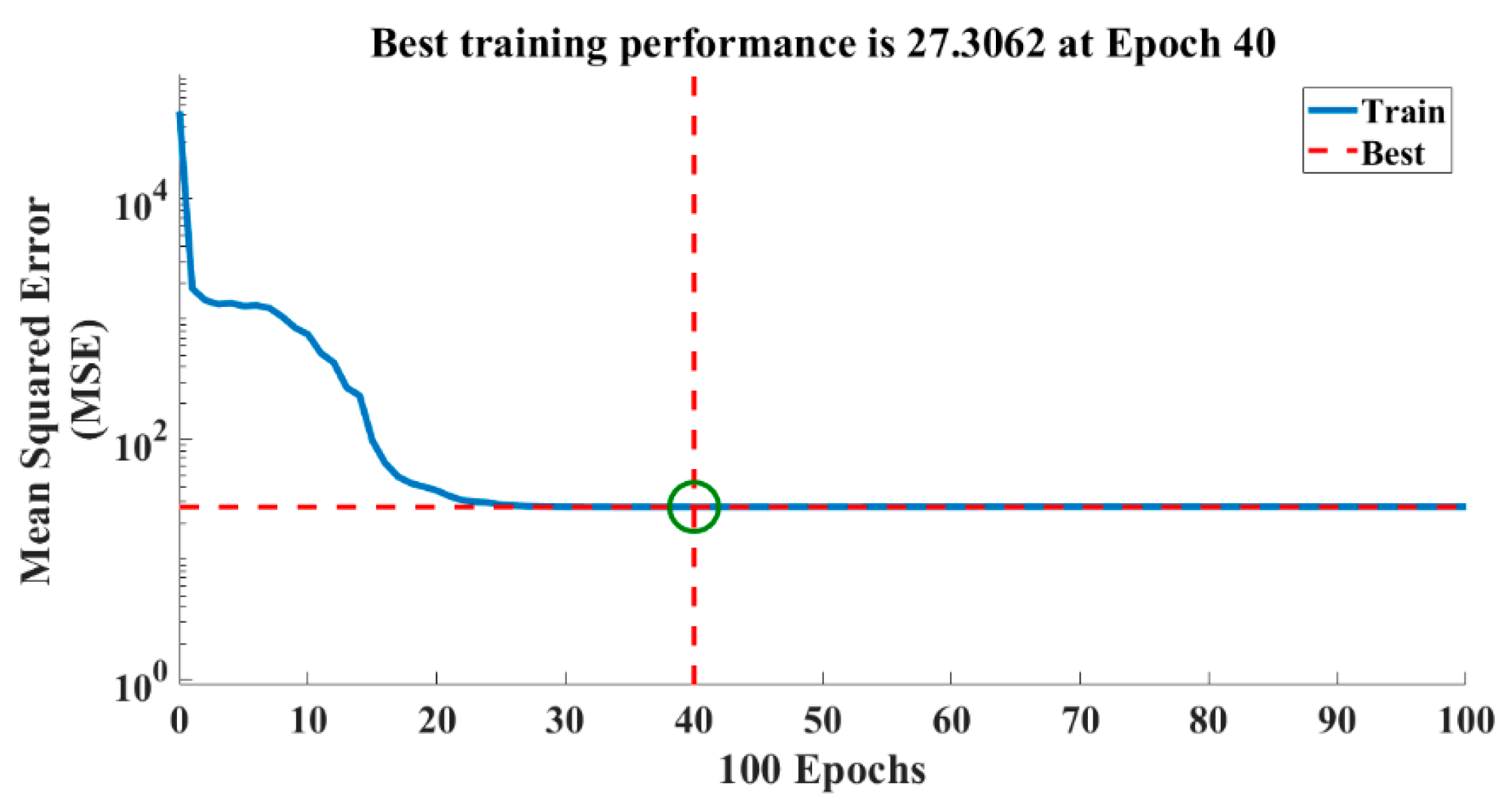
Figure 13.
The reduction of the error with an increase in the number of iterations.
Figure 13.
The reduction of the error with an increase in the number of iterations.
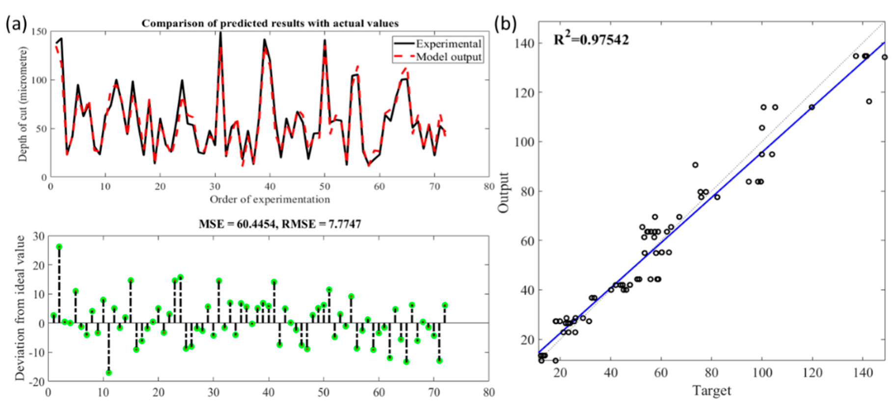
Figure 14.
(a). Comparison of observed and predicted depth of cut using neural network regression; (b) Statistical analysis fit of the neural network regression model.
Figure 14.
(a). Comparison of observed and predicted depth of cut using neural network regression; (b) Statistical analysis fit of the neural network regression model.
Figure 15.
Adaptive Neuro-Fuzzy Inference System (ANFIS) model for belt grinding showing inputs and output [
12].
Figure 15.
Adaptive Neuro-Fuzzy Inference System (ANFIS) model for belt grinding showing inputs and output [
12].
Figure 16.
Change in shape of the Gaussian bell membership function for each input before and after training.
Figure 16.
Change in shape of the Gaussian bell membership function for each input before and after training.
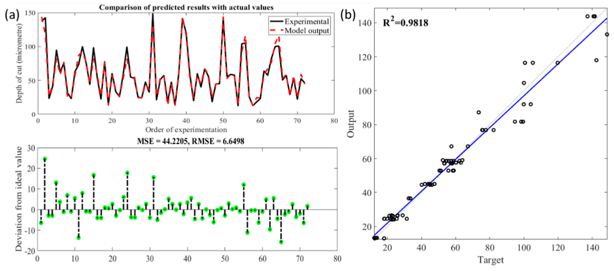
Figure 17.
(a). Comparison of observed and predicted depth of cut using ANFIS with Gaussian bell membership function; (b) Statistical analysis fit of the ANFIS model with Gaussian bell membership.
Figure 17.
(a). Comparison of observed and predicted depth of cut using ANFIS with Gaussian bell membership function; (b) Statistical analysis fit of the ANFIS model with Gaussian bell membership.
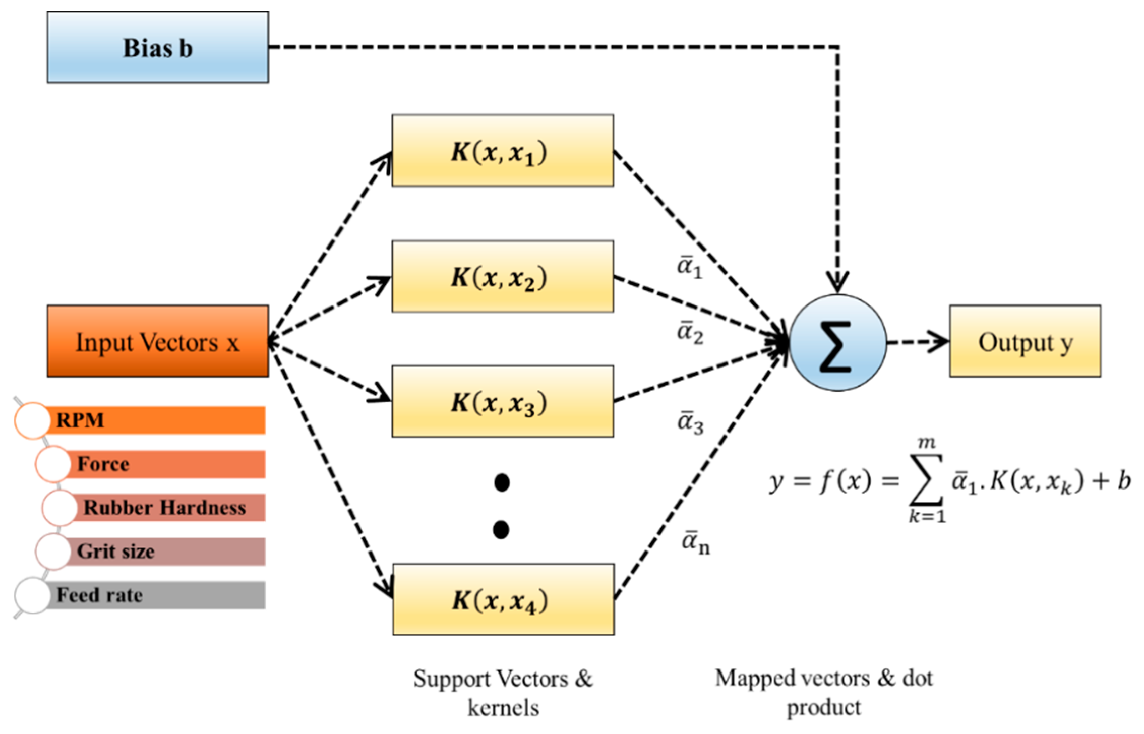
Figure 18.
The architecture of a regression machine constructed by the SVR algorithm.
Figure 18.
The architecture of a regression machine constructed by the SVR algorithm.
Figure 19.
Optimisation of SVR parameters with respect to the number of iterations.
Figure 19.
Optimisation of SVR parameters with respect to the number of iterations.
Figure 20.
(a) Comparison of observed and predicted depth of cut using SVR; (b) Statistical analysis fit of the SVR model.
Figure 20.
(a) Comparison of observed and predicted depth of cut using SVR; (b) Statistical analysis fit of the SVR model.
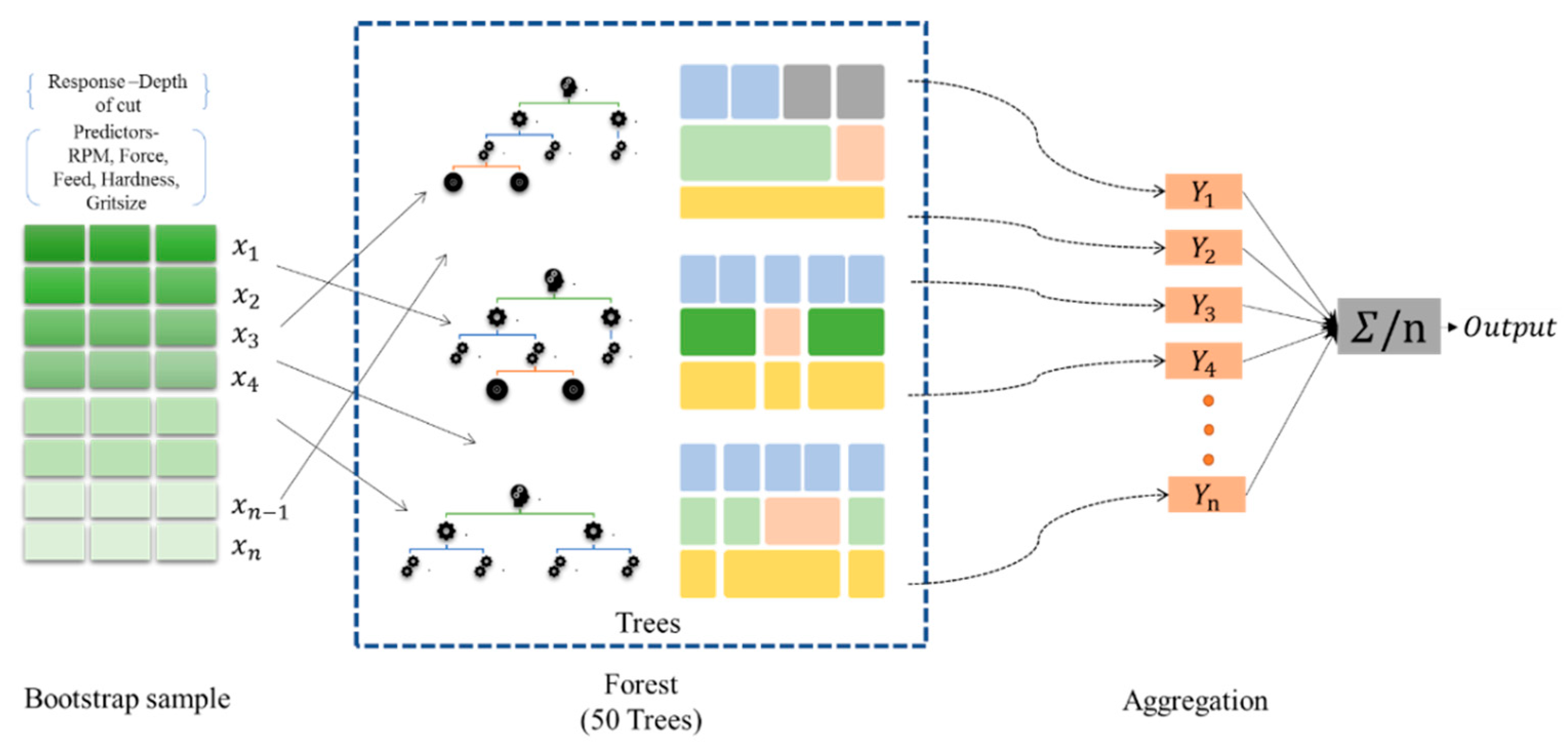
Figure 21.
Material removal prediction using a random forest.
Figure 21.
Material removal prediction using a random forest.
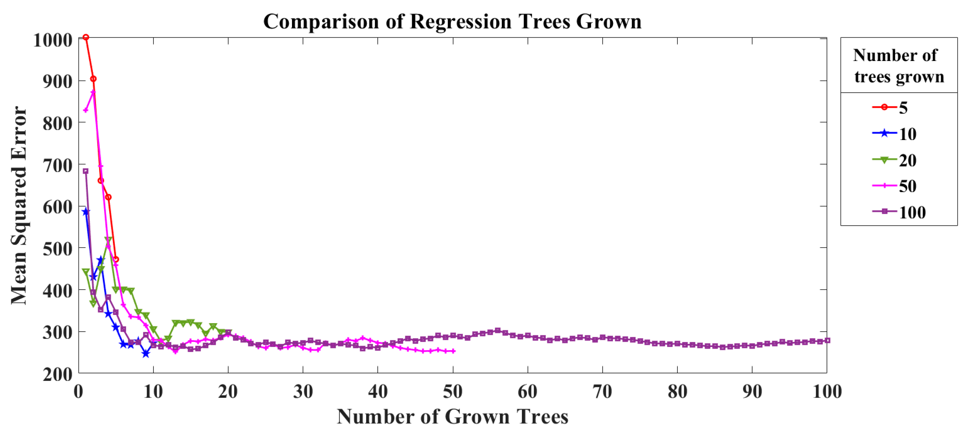
Figure 22.
Optimisation of random forest (RF) parameters (number of grown trees) using mean square error (MSE).
Figure 22.
Optimisation of random forest (RF) parameters (number of grown trees) using mean square error (MSE).
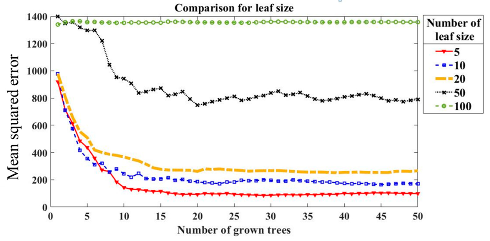
Figure 23.
Optimisation of RF parameters (number of leaf size) using MSE.
Figure 23.
Optimisation of RF parameters (number of leaf size) using MSE.
Figure 24.
Variables’ importance in predicting material removal using RF.
Figure 24.
Variables’ importance in predicting material removal using RF.
Figure 25.
(a). Comparison of observed and predicted depth of cut using RF regression; (b) Statistical analysis fit of the RF regression model.
Figure 25.
(a). Comparison of observed and predicted depth of cut using RF regression; (b) Statistical analysis fit of the RF regression model.
Figure 26.
Predictive performance of the regression models.
Figure 26.
Predictive performance of the regression models.
Table 1.
Research efforts so far in modelling of belt grinding process.
Table 1.
Research efforts so far in modelling of belt grinding process.
| Investigators | Contribution |
|---|
| Y. Wang et al. [13] | Developed a controllable material removal strategy to control the acting force and grinding dwell time by modelling the global and local material removal process of belt grinding. A finite element method (FEM) has been adopted to calculate the local force and global grinding model based on the Hertz contact theory. |
| X. Ren et al. [14] | Established a simulation system using Surfel to visualise the material removal process interactively and to optimise the tool path planning. |
| S. Wu et al. [15] | Presented a comprehensive platform to simulate the belt grinding system incorporating a kinematic model of the robot for tool path planning, dynamic model of the robot joint, along with the material removal model of the grinding process. |
| S. Mezgahani et al. [16] | Performed a comparative study of contact pressure and abrasive grit size to material removal keeping parameters such as speed of workpiece, tool hardness, cycle time, coolant, abrasive feed, and tool wear constant. The study showed that a decrease in grain size results in more ploughing action rather than cutting action. |
| J. Shibata et al. [17] | Offered a metal removal model incorporating the belt wear factor to explain the belt grinding characteristics quantitatively. |
| A. Khellouki et al. [18] | Theoretically modelled contact conditions between abrasive film and the surface and investigated the effect of average contact pressure, contact duration and the number of active grains in the contact. |
| V. T. Thien et al. [19] and Y. Sun et al. [20] | Demonstrated that pressure distribution obtained from pressure films can be correlated with a Hertzian model under different loads and hardness of the polymer wheel. |
| H. Lv et al. [21] | Presented a material removal modelling technique for free-form surface using an echo state network. |
| W. Wang et al. [22] | Proposed a grinding depth predicting frame working using a local stress model and a local material removal model taking into account the contact wheel deformation. |
| Y. Sun et al. [11] and V. Pandiyan et al. [23] | Proposed a novel methodology using a dynamic pressure sensor to predict material removal considering belt grinding parameters such as force, workpiece geometry and different types of contact wheel geometry. |
| Y. J. Wang et al. [24] | Demonstrated that the nonlinear material model performs better than the linear material removal model. |
Table 2.
Belt grinding parameters and their levels.
Table 2.
Belt grinding parameters and their levels.
| Parameter | Unit | Levels |
|---|
| L1 | L2 | L3 |
|---|
| RPM | (m/min) | 250 | 500 | 700 |
| Feed | (mm/s) | 10 | 20 | 30 |
| Force | (N) | 10 | 20 | 30 |
| Rubber hardness | (Shore A) | 30 | 60 | 90 |
| Grit Size | - | 60 | 120 | 220 |
Table 3.
Taguchi design of experiments (DoE) using the L
27 orthogonal array and the corresponding depth of cut [
12].
Table 3.
Taguchi design of experiments (DoE) using the L
27 orthogonal array and the corresponding depth of cut [
12].
| Trial No. | Factors | MRR |
|---|
| RPM | Feed | Force | Hardness | Grit | Depth of Cut |
|---|
| (m/min) | (mm/s) | (N) | (Shore A) | | (μm) |
|---|
| 1 | 250 | 10 | 10 | 30 | 60 | 65.60076 |
| 2 | 250 | 10 | 10 | 30 | 120 | 25.87109 |
| 3 | 250 | 10 | 10 | 30 | 220 | 13.34471 |
| 4 | 250 | 20 | 20 | 60 | 60 | 86.10453 |
| 5 | 250 | 20 | 20 | 60 | 120 | 44.20156 |
| 6 | 250 | 20 | 20 | 60 | 220 | 23.53456 |
| 7 | 250 | 30 | 30 | 90 | 60 | 93.8753 |
| 8 | 250 | 30 | 30 | 90 | 120 | 54.33391 |
| 9 | 250 | 30 | 30 | 90 | 220 | 23.55062 |
| 10 | 500 | 10 | 20 | 90 | 60 | 142.9324 |
| 11 | 500 | 10 | 20 | 90 | 120 | 86.37583 |
| 12 | 500 | 10 | 20 | 90 | 220 | 59.38035 |
| 13 | 500 | 20 | 30 | 30 | 60 | 120.6638 |
| 14 | 500 | 20 | 30 | 30 | 120 | 57.50747 |
| 15 | 500 | 20 | 30 | 30 | 220 | 45.55799 |
| 16 | 500 | 30 | 10 | 60 | 60 | 77.47286 |
| 17 | 500 | 30 | 10 | 60 | 120 | 26.08495 |
| 18 | 500 | 30 | 10 | 60 | 220 | 13.54166 |
| 19 | 700 | 10 | 30 | 60 | 60 | 134.8952 |
| 20 | 700 | 10 | 30 | 60 | 120 | 76.88529 |
| 21 | 700 | 10 | 30 | 60 | 220 | 58.97687 |
| 22 | 700 | 20 | 10 | 90 | 60 | 103.8255 |
| 23 | 700 | 20 | 10 | 90 | 120 | 56.9663 |
| 24 | 700 | 20 | 10 | 90 | 220 | 35.31606 |
| 25 | 700 | 30 | 20 | 30 | 60 | 114.009 |
| 26 | 700 | 30 | 20 | 30 | 120 | 56.65924 |
| 27 | 700 | 30 | 20 | 30 | 220 | 44.31528 |
Table 4.
Stepwise multilinear regression training parameters.
Table 4.
Stepwise multilinear regression training parameters.
| Parameter | Value |
|---|
| Training set | 70% |
| Testing set | 30% |
| Method | Forward stepwise regression |
| Starting model | Linear |
| Upper limit | Quadratic |
Table 5.
Estimated coefficients from stepwise regression.
Table 5.
Estimated coefficients from stepwise regression.
| S. No | Predictors | Estimate | Std Error | t-Stat | p-Value |
|---|
| 1 | (Intercept) | 86.755 | 7.956 | 10.904 | 5.392 × 10⁻²¹ |
| 2 | RPM | 0.049856 | 0.0084825 | 5.8776 | 2.3937 × 10⁻⁸ |
| 3 | Feed | 2.0067 | 0.51282 | 3.9131 | 13.509 × 10⁻⁵ |
| 4 | Force | −2.7861 | 1.2896 | −2.1605 | 03.2243 × 10⁻⁴ |
| 5 | Rubber hardness | 1.7358 | 0.18569 | 9.3481 | 8.2594 × 10⁻¹⁷ |
| 6 | Grit size | −1.3237 | 0.062244 | −21.266 | 3.2042 × 10–48 |
| 7 | RPM: grit size | −0.00014814 | 4.1438 × 10⁻⁵ | −3.575 | 4.6498 × 10⁻⁴ |
| 8 | Feed: force | 0.062239 | 0.011008 | 5.654 | 7.1536 × 10⁻⁸ |
| 9 | Feed: rubber hardness | −0.069002 | 0.0091514 | −7.5401 | 3.4527 × 10⁻¹² |
| 10 | Force: grit size | −0.0035275 | 0.00096854 | −3.642 | 3.6624 × 10⁻⁴ |
| 11 | Rubber hardness: grit size | −0.0010501 | 0.00031645 | −3.3184 | 1.1237 × 10⁻³ |
| 12 | Force^2 | 0.084463 | 0.029849 | 2.8297 | 5.265 × 10⁻³ |
| 13 | Grit size^2 | 0.0039407 | 0.00018283 | 21.554 | 6.5639 × 10–49 |
Table 6.
ANN training algorithm configuration parameters.
Table 6.
ANN training algorithm configuration parameters.
| Parameter | Value |
|---|
| Maximum number of epochs to train | 200 |
| Performance goal | 0 |
| Backpropagation method | Bayesian regularisation |
| Initial μ | 0.005 |
| Hidden layers | 10, 20, 30 |
| Training | 70% of the dataset |
| Testing | 30% of the dataset |
| Weight function | Dot product |
| Activation function | tansig |
| Predictors | 5 |
| Response | 1 |
Table 7.
Comparison of hidden layers against epochs to reach the performance goal.
Table 7.
Comparison of hidden layers against epochs to reach the performance goal.
| Hidden Layers | Epochs |
|---|
| 10 | 151 |
| 20 | 62 |
| 30 | 40 |
Table 8.
The ANFIS training parameters with four different membership functions.
Table 8.
The ANFIS training parameters with four different membership functions.
| Parameter | Value |
|---|
| andMethod | Prod |
| orMethod | Max |
| defuzzMethod | Wtaver (Weighted average) |
| impMethod | Prod |
| aggMethod | Max |
| Membership function | /Sigmoidal/Gaussian bell/Gaussian/Bell-shaped |
| Learning rules | Gradient descent algorithm |
Table 9.
Comparison of prediction accuracy and membership function.
Table 9.
Comparison of prediction accuracy and membership function.
| Membership Function | RMSE |
|---|
| Sigmoidal membership [12] | 5.648 |
| Gaussian bell membership | 6.7941 |
| Gaussian membership | 7.100 |
| Bell-shaped membership | 7.0341 |
Table 10.
Optimised SVR training parameters.
Table 10.
Optimised SVR training parameters.
| Parameter | Value |
|---|
| Epsilon () | 0.12457 |
| Box Constraint (C) | 989.65 |
| Optimisation Method | Bayesian optimisation |
| Kernel | Gaussian RBF |
| Kernel scale () | 0.10894 |
Table 11.
Random forest training parameters.
Table 11.
Random forest training parameters.
| Parameter | Value |
|---|
| In bag fraction | 0.25% of the training dataset |
| Method used by trees | Regression |
| Min leaf size | 5 |
| Number of trees | 50 |


