A Feasible Temporal Links Prediction Framework Combining with Improved Gravity Model

Abstract

Social network analysis is a multidisciplinary study covering informatics, mathematics, sociology, management, psychology, etc. Link prediction, as one of the fundamental studies with a variety of applications, has attracted increasing focus from scientific society. Traditional research based on graph theory has made numerous achievements, whereas suffering from incapability of dealing with dynamic behaviors and low predicting accuracy. Aiming at addressing the problem, this paper employs a diagonally symmetrical supra-adjacency matrix to represent the dynamic social networks, and proposes a temporal links prediction framework combining with an improved gravity model. Extensive experiments on several real-world datasets verified the superiority on competitors, which benefits recommending friends in social networks. It is of remarkable significance in revealing the evolutions in temporal networks and promoting considerable commercial interest for social applications.

1. Introduction

The analysis of social networks has drawn increasing attention in the field of sociology. It analyzes and explores the potential relations between social objects [1]. The rapid development of social media has brought us plentiful data sources, along with enormous challenges such as data incompletion and dynamic changes [2]. On the one hand, researchers are facing data incompletion problem since only part of social information can be collected from social platforms. On the other hand, the dynamic changes may lead the nodes and links to appear and disappear in the future, which makes the underlying graph longitudinal [3].

Link prediction [4], as fundamental research in social network analysis, is proposed to detect unobserved links from existing parts of the network [5] or forecast future links from current network structures [6]. The former research, also known as missing links prediction, has been fruitful during the last decade, whereas the prediction of future links is more challenging to estimate the upcoming connections with limited social information. This study is of great importance, not only in revealing the evolution of social networks, but also benefiting network management, such as promoting useful links or prohibiting harmful interactions. For instance, a recommendation system [7], as a typical application of temporal links prediction, is designed for individuals to make friends or purchase goods via efficient predicted results, which brings considerable benefits for corporations.

Numerous attempts have been made to address the problem of temporal links prediction, but it is a really difficult task. Firstly, the observed social information is quite limited, which leads to the smoothness assumption [8] being frequently adopted in studies, thereby the methods may be incapable when the network changes seriously. Secondly, longitudinal bias is inevitable, as the dynamic changes must be shifted towards future [3]. Finally, the different observation of extensive network changes over time may also lead to various social structures, which may yield extremely different predicting results. To solve the problem of temporal links prediction, this paper proposes a dynamic similarity framework with an improved gravity model to estimate the future links in temporal networks.

The rest of this paper is organized as follows. Section 2 introduces the related works on link prediction. Section 3 presents the mathematical model, the improved gravity model, and the framework for predicting temporal links. Section 4 presents the experiments and analysis, including comparison experiments on real-world dataset separated by different levels, which verified the feasibility and veracity of the method. Section 5 summarizes the whole paper and provides concluding remarks.

2. Related Works

Link prediction was first proposed on SIGKDD in 2005 [4]. Afterwards, Liben-Nowell and Kleinber reviewed the link prediction in social networks, which attracted more and more scholars devoting themselves to this field [9]. In 2011, Lü summarized the existing methods and classified them into three categories: structure similarity index, maximum likelihood approximation, and probabilistic model [10]. In 2017, Pech et al. [11] introduced robust principal component analysis (robust PCA) method into link prediction and estimated the missing links of the adjacency matrix. Experimental results show that, when the target network is connected and sufficiently dense, the proposed method achieves much higher accuracy compared of some the state-of-the-art algorithms. A brief summary of the classic predicators is shown in Table 1.

The prediction of future links [12,13], i.e., temporal links prediction, aims to predict the links in a network that would appear in the next state of period. As for temporal networks, a series of mathematic models are proposed, such as temporal graphs [14], evolving graphs [15], time-varying graphs, dynamic networks [16], etc. Three representative models are available to depict dynamic behaviors: Snapshots, Contact sequences and Interval graphs.

Snapshots, as a favorable model to exhibit dynamic behaviors, have been widely used in various application scenarios. By employing such representation, unsupervised learning methods are feasible to estimate the links at time t with the observed network structures at time $[1,t-1]$ [17,18,19]. Besides, statistical methods, such as Exponential Smoothing (EPS) [20] and Autoregressive Integrated Moving Average(ARIMA) [21], are also employed to predict temporal links with snapshots representation. However, Snapshots suffer from coarse-grained depiction of continuous changes, which probability result in poor predictive performance and misleading results [22]. Distinguished by the duration of interaction being negligible or not, Contact sequences and Interval graphs are proposed to illustrate the network dynamics. A temporal network can be represented by a series of triplet $(i,j,t)$ where i and j are entities and t is the time of interaction. If the duration of interaction is not negligible, the framework can be represented by $(i,j)$ = $(t_1,{t^{\prime }}_1),\dots ,(t_n,{t^{\prime }}_n)$, namely Interval graphs. Although they encode more interactions information of dynamic behaviors, the above-mentioned two models are scarcely used in studying temporal link prediction for their complicated expressions.

By combining with temporal correlations and evolutions of link occurrences, Özcan and Öǧüdücü [23] proposed Multivariate Time Series Link Prediction method. Experiments on real-world bibliographic datasets showed that the proposed method, which can incorporate covariance structures, achieved better results for temporal links prediction than classic competitors. Considering both temporal dynamics and multi-relational properties in bibliographic networks, Sett et al. [3] proposed a robust and efficient set of features named time-aware multi-relational link prediction (TMLP) features to predict future links using supervised learning framework in dynamic multi-relational network. They analyzed unsupervised performance of individual features, and then applied a supervised learning method that combines multiple features towards link prediction. To overcome the inherent problem of longitudinal bias, random forests supervised learning framework is utilized in the experiments. Experiments on bibliographic datasets showed the effectiveness. However, the above-mentioned methods rely on the plentiful data features and the performance on general temporal network is uncertain. Overall, the study on temporal links prediction is blossoming and still requires great endeavors to achieve better performance.

Table 1. A brief summary of the existing link prediction methods.

Indicator	Topology	Definition 1	Complexity 2
CN [24]	Local	$S_{xy}=|\Gamma \left(x\right)\cap \Gamma \left(y\right)|$	$O\left(n^2\right)$
Salton [25]	Local	$S_{xy}=\frac{|\Gamma (x)\cap \Gamma (y\left)\right|}{\sqrt{k_x{k}_y}}$	$O\left(n^2\right)$
Jaccard [26]	Local	$S_{xy}=\frac{|\Gamma (x)\cap \Gamma (y\left)\right|}{|\Gamma (x)\cup \Gamma (y\left)\right|}$	$O\left(2n^2\right)$
Sorenson [27]	Local	$S_{xy}=\frac{2\times |\Gamma (x)\cap \Gamma (y\left)\right|}{k_x+k_y}$	$O\left(n^2\right)$
HPI [28]	Local	$S_{xy}=\frac{|\Gamma (x)\cap \Gamma (y\left)\right|}{min(k_x,k_y)}$	$O\left(n^2\right)$
HDI [29]	Local	$S_{xy}=\frac{|\Gamma (x)\cap \Gamma (y\left)\right|}{max(k_x,k_y)}$	$O\left(n^2\right)$
LHN-I [29]	Local	$S_{xy}=\frac{|\Gamma (x)\cap \Gamma (y\left)\right|}{k_x,k_y}$	$O\left(n^2\right)$
AA [30]	Local	$S_{xy}={\sum }_{z\in \Gamma \left(x\right)\cap \Gamma \left(y\right)}\frac{1}{log{k}_z}$	$O\left(2n^2\right)$
RA [31]	Local	$S_{xy}={\sum }_{z\in \Gamma \left(x\right)\cap \Gamma \left(y\right)}\frac{1}{k_z}$	$O\left(2n^2\right)$
PA [32]	Local	$S_{xy}=k_x{k}_y$	$O\left(2n\right)$
LP [33]	Semi-Local	$S=A^2+\alpha ·A^3$	$O\left(n^3\right)$
Katz [34]	Global	$S={(I-\alpha ·A)}^{-1}-I$	$O\left(n^3\right)$
LHN-II [35]	Global	$S=2m{\lambda }_1{D}^{-1}{(I-\frac{\varphi }{{\lambda }_1})}^{-1}{D}^{-1}$	$O\left(n^3\right)$
LRW [36]	Semi-Local	$S_{xy}^{LRW}\left(t\right)=q_x·{\pi }_{xy}\left(t\right)+q_y·{\pi }_{yx}\left(t\right)$	$O\left(n{k}^t\right)$
SRW [36]	Semi-Local	$S_{xy}^{SRW}\left(t\right)={\sum }_{l=1}^t{S}_{xy}^{LRW}\left(l\right)=q_x{\sum }_{l=1}^t{\pi }_{xy}\left(l\right)+q_y{\sum }_{l=1}^t{\pi }_{yx}\left(l\right)$	$O\left(n{k}^t\right)$
RWR [37]	Semi-Local	$S_{xy}^{LRW}\left(t\right)=q_{xy}+q_{yx}$	$O\left(n^3\right)$
ACT [38]	Semi-Local	$S_{xy}^{ACT}=\frac{1}{l_{xx}^{+}·l_{yy}^{+}-2l_{xy}^{+}}$	$O\left(n^3\right)$
SimR [39]	Global	$S_{xy}^{SimR}=C\frac{{\sum }_{v_z\in \Gamma \left(x\right)}{\sum }_{v_{z^{\prime }}\in \Gamma \left(y\right)}{S}_{z{z}^{\prime }}^{SimR}}{k_x{k}_y}$	$O\left(n^3\right)$
Cos+ [40]	Semi-Local	$S_{xy}^{cos+}=cos{(x,y)}^{+}=\frac{l_{xy}^{+}}{\sqrt{l_{xx}^{+}·l_{yy}^{+}}}$	$O\left(n^3\right)$
TS [41]	Global	$S^{Tr}={(I-\epsilon S)}^{-1}S$	$O\left(n^3\right)$
LowRank [11]	Global	$S={min}_{X^{*},E}\left|\right|X^{*}{\left|\right|}_{*}+\lambda {\left|\right|E\left|\right|}_1$	$O\left(n{k}^3\right)$
MFI [42]	Global	$S={(I+\alpha ·L)}^{-1},\alpha >0$	$O\left(n^3\right)$

¹$\Gamma \left(x\right)$ and $\Gamma \left(y\right)$ denote the neighbors of node x and y, respectively; $k_x$ and $k_y$ are the degrees of node x and y, respectively; m is the number of edges; $l_{xy}^{+}$ denotes the element at row x, column y of the pseudo-inverse matrix $L^{+}$; $q_{xy}$ represents the probability of random walk from node x to node y; $\epsilon$ represents an adjustable parameter; ${\pi }_{xy}\left(l\right)$ is the random walk probability from node x to node y at time l; ² n denotes the number of nodes; k is the average degree of nodes; and t is the step of random walk steps.

Table 1. A brief summary of the existing link prediction methods.

Indicator	Topology	Definition 1	Complexity 2
CN [24]	Local	$S_{xy}=|\Gamma \left(x\right)\cap \Gamma \left(y\right)|$	$O\left(n^2\right)$
Salton [25]	Local	$S_{xy}=\frac{|\Gamma (x)\cap \Gamma (y\left)\right|}{\sqrt{k_x{k}_y}}$	$O\left(n^2\right)$
Jaccard [26]	Local	$S_{xy}=\frac{|\Gamma (x)\cap \Gamma (y\left)\right|}{|\Gamma (x)\cup \Gamma (y\left)\right|}$	$O\left(2n^2\right)$
Sorenson [27]	Local	$S_{xy}=\frac{2\times |\Gamma (x)\cap \Gamma (y\left)\right|}{k_x+k_y}$	$O\left(n^2\right)$
HPI [28]	Local	$S_{xy}=\frac{|\Gamma (x)\cap \Gamma (y\left)\right|}{min(k_x,k_y)}$	$O\left(n^2\right)$
HDI [29]	Local	$S_{xy}=\frac{|\Gamma (x)\cap \Gamma (y\left)\right|}{max(k_x,k_y)}$	$O\left(n^2\right)$
LHN-I [29]	Local	$S_{xy}=\frac{|\Gamma (x)\cap \Gamma (y\left)\right|}{k_x,k_y}$	$O\left(n^2\right)$
AA [30]	Local	$S_{xy}={\sum }_{z\in \Gamma \left(x\right)\cap \Gamma \left(y\right)}\frac{1}{log{k}_z}$	$O\left(2n^2\right)$
RA [31]	Local	$S_{xy}={\sum }_{z\in \Gamma \left(x\right)\cap \Gamma \left(y\right)}\frac{1}{k_z}$	$O\left(2n^2\right)$
PA [32]	Local	$S_{xy}=k_x{k}_y$	$O\left(2n\right)$
LP [33]	Semi-Local	$S=A^2+\alpha ·A^3$	$O\left(n^3\right)$
Katz [34]	Global	$S={(I-\alpha ·A)}^{-1}-I$	$O\left(n^3\right)$
LHN-II [35]	Global	$S=2m{\lambda }_1{D}^{-1}{(I-\frac{\varphi }{{\lambda }_1})}^{-1}{D}^{-1}$	$O\left(n^3\right)$
LRW [36]	Semi-Local	$S_{xy}^{LRW}\left(t\right)=q_x·{\pi }_{xy}\left(t\right)+q_y·{\pi }_{yx}\left(t\right)$	$O\left(n{k}^t\right)$
SRW [36]	Semi-Local	$S_{xy}^{SRW}\left(t\right)={\sum }_{l=1}^t{S}_{xy}^{LRW}\left(l\right)=q_x{\sum }_{l=1}^t{\pi }_{xy}\left(l\right)+q_y{\sum }_{l=1}^t{\pi }_{yx}\left(l\right)$	$O\left(n{k}^t\right)$
RWR [37]	Semi-Local	$S_{xy}^{LRW}\left(t\right)=q_{xy}+q_{yx}$	$O\left(n^3\right)$
ACT [38]	Semi-Local	$S_{xy}^{ACT}=\frac{1}{l_{xx}^{+}·l_{yy}^{+}-2l_{xy}^{+}}$	$O\left(n^3\right)$
SimR [39]	Global	$S_{xy}^{SimR}=C\frac{{\sum }_{v_z\in \Gamma \left(x\right)}{\sum }_{v_{z^{\prime }}\in \Gamma \left(y\right)}{S}_{z{z}^{\prime }}^{SimR}}{k_x{k}_y}$	$O\left(n^3\right)$
Cos+ [40]	Semi-Local	$S_{xy}^{cos+}=cos{(x,y)}^{+}=\frac{l_{xy}^{+}}{\sqrt{l_{xx}^{+}·l_{yy}^{+}}}$	$O\left(n^3\right)$
TS [41]	Global	$S^{Tr}={(I-\epsilon S)}^{-1}S$	$O\left(n^3\right)$
LowRank [11]	Global	$S={min}_{X^{*},E}\left|\right|X^{*}{\left|\right|}_{*}+\lambda {\left|\right|E\left|\right|}_1$	$O\left(n{k}^3\right)$
MFI [42]	Global	$S={(I+\alpha ·L)}^{-1},\alpha >0$	$O\left(n^3\right)$

¹$\Gamma \left(x\right)$ and $\Gamma \left(y\right)$ denote the neighbors of node x and y, respectively; $k_x$ and $k_y$ are the degrees of node x and y, respectively; m is the number of edges; $l_{xy}^{+}$ denotes the element at row x, column y of the pseudo-inverse matrix $L^{+}$; $q_{xy}$ represents the probability of random walk from node x to node y; $\epsilon$ represents an adjustable parameter; ${\pi }_{xy}\left(l\right)$ is the random walk probability from node x to node y at time l; ² n denotes the number of nodes; k is the average degree of nodes; and t is the step of random walk steps.

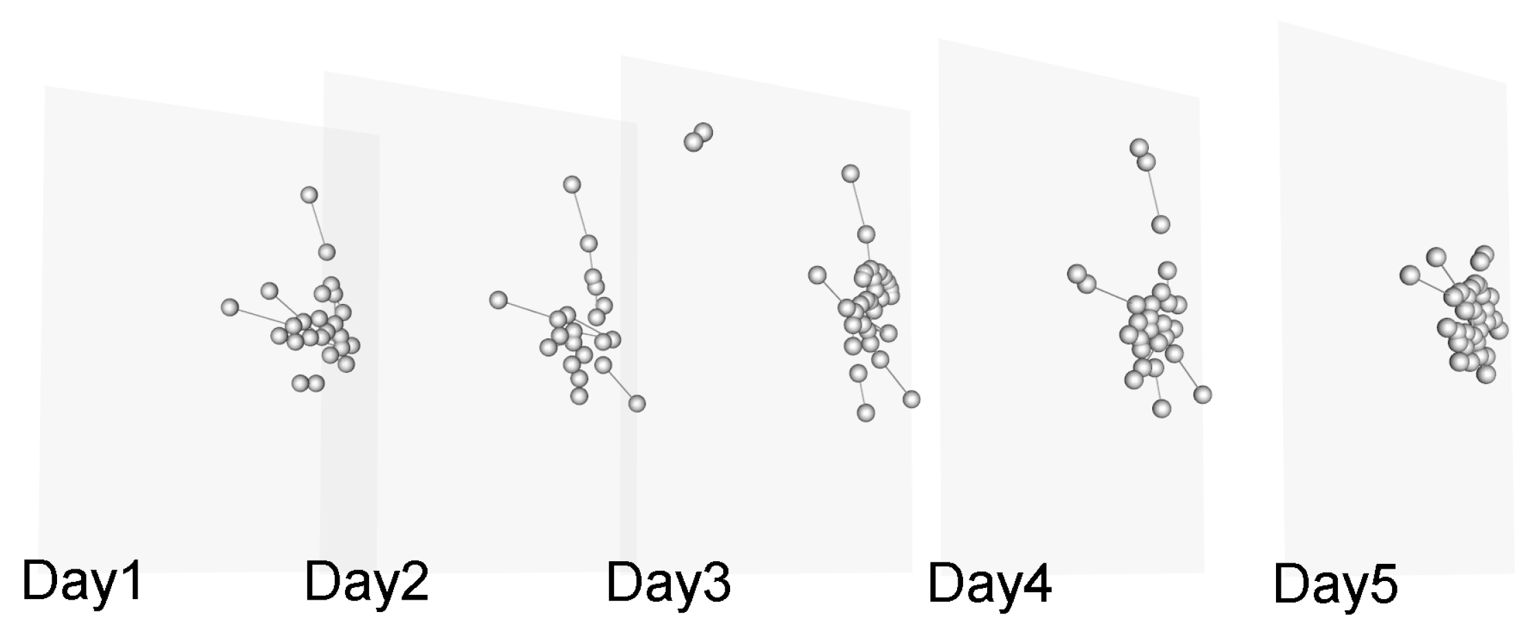
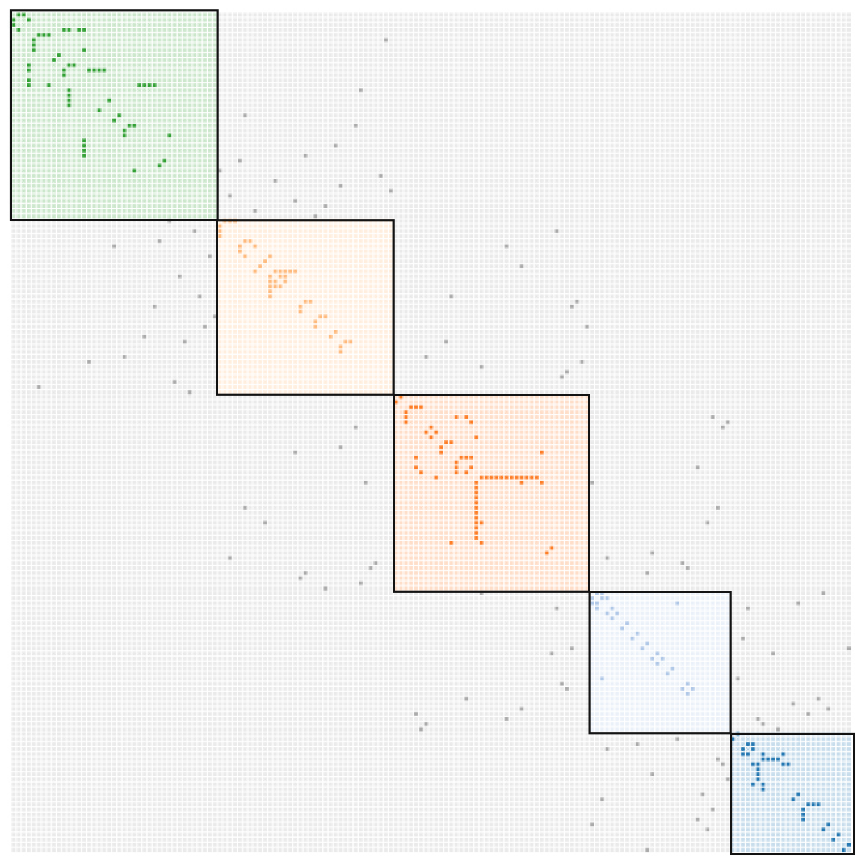
3. Modeling and Methods

3.1. Model

The problem of link prediction is described as estimating the likelihood of all the possible links with a given network model $G=(V,E)$, where $V=\{v_1,v_2,\dots ,v_n\}$ is the node set and $E=\left\{(v_i,v_j)\right\}$, ($v_i$, $v_j\in V$) is the edge set. Suppose the likelihood (or similarity) of the link between every two nodes in G can be calculated by a certain algorithm, and then sorted by ascending order; the future links are obtained by top-k links, where k is the target links amount.

In this paper, we employ a generative multilayer network model [43], which can transform the temporal network into a considerable collection of snapshots. An illustration of the multilayer network model with data derived from a large European research institution [44] is shown in Figure 1 and the corresponding supra-adjacency matrix is shown in Figure 2.

Suppose given a temporal network $G^T$ with T separated slices, where each slice is modeled as a mono-layer network (i.e., single-layer network), T is the total number of layers, and $t=1,2,\dots ,T$; the model is denoted by

$$G^T=\{\sum V^t,\sum E^t\},$$

(1)

where $\sum V^t$ and $\sum E^t$ are the union of the nodes and edges at each slice. To simplify the research problem, we utilize undirected graph to present the network structures in each snapshot. Thus, the temporal network can be represented by a diagonally symmetrical supra-adjacency matrix (denoted by $\tilde{M}$), described as

$$\tilde{M}=\left[\begin{array}{ccc}{A}_1& I_{1,2}& \\ I_{2,1}& A_2& \ddots & \\ & \ddots & \ddots & I_{T-1,T}\\ & & I_{T,T-1}& A_T\end{array}\right]\in {\mathcal{R}}^{N\times N},$$

(2)

where $A_1$, $A_2$, …, $A_T$ are the adjacency matrix of time 1, 2, …, T, respectively, representing the links (i.e., intra-layer edges). N is the total numbers of the nodes, which can be calculated by $N={\sum }_{1\le l\le T}\left|V^l\right|$. I denotes the relationship of the node located in the continuous snapshots (i.e., the inter-layer edges). By utilizing the former temporal information from time 1 to $T-1$, our goal is to predict the links at the last time T. The problem is described as

$$P_{(u,v)}\otimes T=\sum _{1\le t\le T-1}\tau (p_{(u,v)}\otimes t)·E_{(u,v)}\otimes t,$$

(3)

where $P_{(u,v)}\otimes T$ is the predicted likelihood of link connected node u and v at time T, $p_{(u,v)}\otimes t$ is the likelihood indicator of node u and v at time t, $\tau$ depicts the varying function of determining the influence at different time t and $E_{(u,v)}\otimes t$ is the existence function of nodes u and v at time t, described as

$$E_{(u,v)}\otimes t=\left\{\begin{array}{cc}\sum I_u{I}_v,\hfill & \mathrm{if}\mathrm{node}u\mathrm{links}v\mathrm{at}\mathrm{time}t\hfill \\ 0,\hfill & \mathrm{otherwise}\hfill \end{array}\right.,$$

(4)

where $I_u$ and $I_v$ represent the interlayer edges of node u and v, respectively. The prediction of future links (at time T) relies on the former structures (i.e., from time 1 to time $T-1$). The links with the maximum score are the prediction results of future links. The prediction result is evaluated by precision, recall, $F_{1-\mathrm{value}}$, accuracy, etc. Considering the significance of prediction, AUC [45] is employed for evaluation in this paper.

3.2. Definitions

Gravity is the force between objects, which relates to the qualities of the objects and the distance between the two objects. The gravity we focus on in this paper is utilized to describe the strength of the interactions between the two nodes. The gravity in networks [46] is defined as

$$G_{i,j}=\frac{k_i·k_j}{d_{ij}^2},$$

(5)

where $G_{i,j}$ represents the gravity between node i and j, $d_{ij}$ depicts the shortest path length between node i and node j, and $k_i$ is the degree of node i. Inspired by this model, we simplify the time-consuming process, namely the calculation of shortest path, by merely considering the neighbors within two steps (i.e., neighbors and second-order neighbors), denoted by GR. Thus, it can be reduced to the accumulation of gravity between common neighbors, and the likelihood of existing links between node i and j is given by

$$S_{i,j}^{GR}=\sum _{z\in \Gamma \left(i\right)\cap \Gamma \left(j\right)}{\displaystyle \frac{G_{i,z}·G_{z,j}}{{\delta }^2}},$$

(6)

where $\Gamma \left(i\right)$ and $\Gamma \left(j\right)$ are the neighbors of node i and node j, respectively. $\delta$ is the steps between node i and j if there are common neighbors between i and j, and the number of nodes otherwise. Thus, the predicted likelihood of node i and j at time t (marked as $S_{i,j}^{GR}\otimes T$) is given by

$$S_{i,j}^{GR}\otimes T=\sum _{t=0}^{t-1}{G}_{i,j}^{GR|t}\times e^{-\alpha (t-p)},$$

(7)

where $G_{i,j}^{GR|t}$ is the gravity of node i and j at time t. $e^{\alpha (t-p)}$ is the above-mentioned $\tau$ function to enforce temporal effect on the similarity evaluation [47], namely dynamic similarity process (for short DS). p is the existence duration of i and j. $\alpha$ is the attenuation constant in the range of [0, 1]. The values change with x under different $\alpha$, as shown in Figure 3.

Suppose k is the number of links to be predicted in the future. The algorithm of predicting future links is described as the following steps.

Step 1: Obtain all the node pairs at $T-1$ layer as the target-predicting links.

Step 2: Collect all the existing links from the start time to time $T-1$, marked as training set.

Step 3: Calculate the likelihood of node pairs in the training set in terms of Equation (7).

Step 4: Sort the possible links in descending order and obtain the top-k results as the predicted result.

The pseudo-code of the above process is shown as Algorithm 1.

Algorithm 1: Temporal links prediction framework.

3.3. Complexity Analysis

Suppose m and n are the number of edges and nodes, respectively, the average degree of nodes is d, and the total layers of temporal networks is T. The complexity of calculating common neighbors is $O\left(d^2\right)$. Thus, the complexity of the proposed indicator $S_{i,j}^{GR}$ is lower than $O(d^2+d)$, which can be simplified as $O\left(d^2\right)$. Traversing every two nodes at time $T-1$ needs complexity of $O\left(n^2\right)$, thus the total complexity is $O\left(n^2{d}^2\right)$. Actually, $d^2$ is much smaller than n, thus the proposed method can be simplified as $O\left(n^2\right)$. It is very close to competitive indicators, e.g., CN, AA, and RA are all with complexity of $O\left(n^2\right)$ [48]. The process of temporal links prediction our method $S_{i,j}^{GR}\otimes T$ is $O\left(n^{2}T\right)$, which is the same as the representative Linear Regression methods, EPS [20], and so on.

4. Experiments and Discussion

The experimental environment was a Intel(R) Core (TM) i5-7200U CPU @ 2.50 GHz (4 CPUs), 2.7 GHz, the memory was 8 GB DDR3, the operating system was Windows10 64 bit, the programming language was Python 3.7.1, and the relevant libs were NetworkX 2.2 and Multinetx. The goal of the experiments was to validate the performance of the proposed method and compare with competitive indicators.

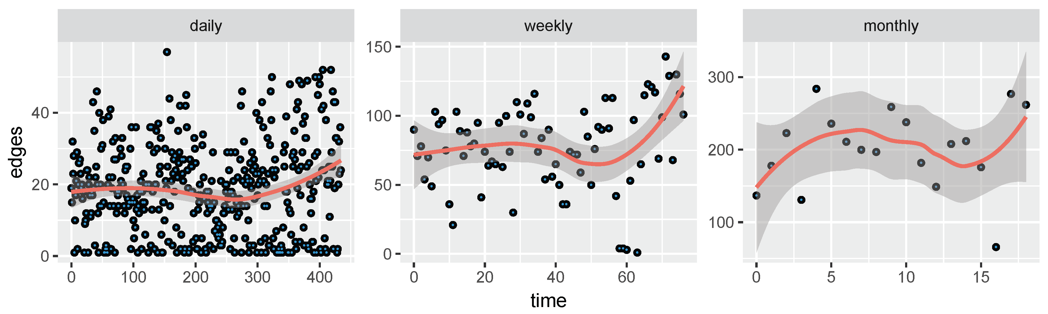
4.1. Experimental Datasets

To verify the proposed indicator, seven real-world datasets were employed in the experiments, as shown in

Table 2. Statistics of seven real-world datasets.

Dataset Name	$\left|\mathit{V}\right|$	|E|	<k>	|C|	<c>	|D|	r
Zachary karate Club [49]	34	78	4.59	0.57	2.41	2.22	−0.48
Dolphins social network [50]	62	159	5.13	0.26	3.06	3.36	−0.04
Terriers of 9/11 [51]	69	159	4.61	0.47	1.76	3.22	−0.04
NEUSNCP dataset 1	89	365	4.10	0.54	3.15	1.92	−0.40
Books about US politics [52]	105	411	8.40	0.49	5.26	3.08	−0.13
American college football network [53]	115	613	10.66	0.40	10.23	2.51	0.16
Scientist collaboration network [52]	1589	2742	4.60	0.64	0.08	5.99	−0.09

Note:$\left|V\right|$ denotes the number of nodes; $\left|E\right|$ denotes the number of edges; <k> is the average degree; $\left|C\right|$ is the average clustering index; <c> is the average connectivity; $\left|D\right|$ is the average shortest path; and r represents assortativity coefficient. ¹ We developed an experimental social platform and invited hundreds of users to register. Data availability: https://www.neusncp.com/api/about.

. The real-world email dataset from a large European research institution [44] was employed to check the proposed dynamic similarity framework and the data statistics are shown in

Table 3. Data statistics of Email-Eu-core temporal network.

Dataset Name	$\left|\mathit{V}\right|$	$\left|\mathit{E}\right|$	Days
Email-Eu-core temporal network	986	332,334	803
Email-Eu-core-temporal-Dept1	309	61,046	803
Email-Eu-core-temporal-Dept2	162	46,772	803
Email-Eu-core-temporal-Dept3	89	12,216	803
Email-Eu-core-temporal-Dept4	142	48,141	803

.

The email dataset is convictive without providing any feature information. The e-mails only represent communication between institution members (the core), and the dataset does not contain incoming messages from or outgoing messages to the rest of the world. To illustrate the connections of each period, the dataset was separated by different intervals (daily, weekly, and monthly), as shown in Figure 4.

As shown in Figure 4, the more layers there are in the multilayer network model, the fewer connections there are in each slice. The fitting results of connections are marked with red lines in the above three panels. Here, we can see the number of edges is varying over time among all three separations. When the dataset is daily separated, the fitting result is not obvious and indicates poor predictive performance. When the dataset is weekly separated, the improved fitting result provides a better predictive training set. When the dataset is monthly separated, an obvious fitting seems to reveal a better predictive result.

4.2. Performance Comparison

First, we compared the proposed GR indicator with several classic methods. The results were evaluated by AUC via the average result of 100 independent experiments, as shown in

Table 4. AUC of the GR and other indicators comparison.

Dataset Name	GR	AA	RA	JC	PA	CN
Zachary karate Club	0.8790	0.8784	0.8784	0.6281	0.8773	0.8433
Dolphins social network	0.7442	0.7428	0.7425	0.7431	0.6621	0.7379
Terriers of 9/11	0.9374	0.9339	0.9371	0.9151	0.7144	0.9103
NEUSNCP dataset	0.9110	0.9105	0.9096	0.8855	0.6725	0.9012
Books about US politics	0.8310	0.8299	0.8299	0.8397	0.2573	0.8304
American college football network	0.8775	0.8750	0.8769	0.7494	0.8381	0.8657
Scientist collaboration network	0.9431	0.9431	0.9431	0.9430	0.6725	0.9429

.

Table 4 shows that the AUC obtained by the proposed GR indicator generally outperforms the competitive methods, as marked by boldface. Although the performance of GR on Books about US politics dataset is inferior to that of JC indicator, it is still competitive. Generally, the experiments verified the performance of the proposed indicator in predicting unknown links.

Secondly, we compared the proposed method with the existing linear regression method, ARIMA, EPS methods, and the AUC results of six indicators are shown in Figure 5.

Obviously, the result of temporal links prediction obtained from our proposed method (DS combined with GR indicator) outperforms the competitive methods. When the datasets were daily separated, the proposed method obtained maximum AUC, achieving 0.913 and 0.8444 when weekly and monthly separated, respectively, which are greater than the result of the other methods.

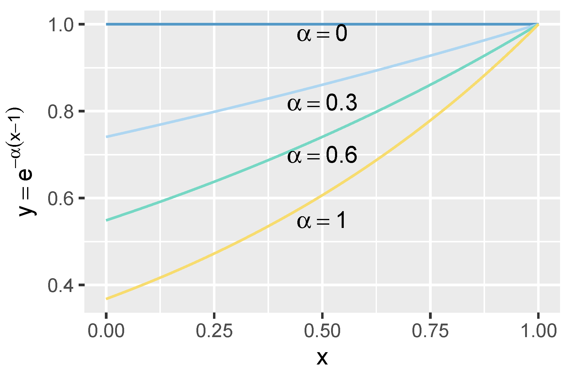
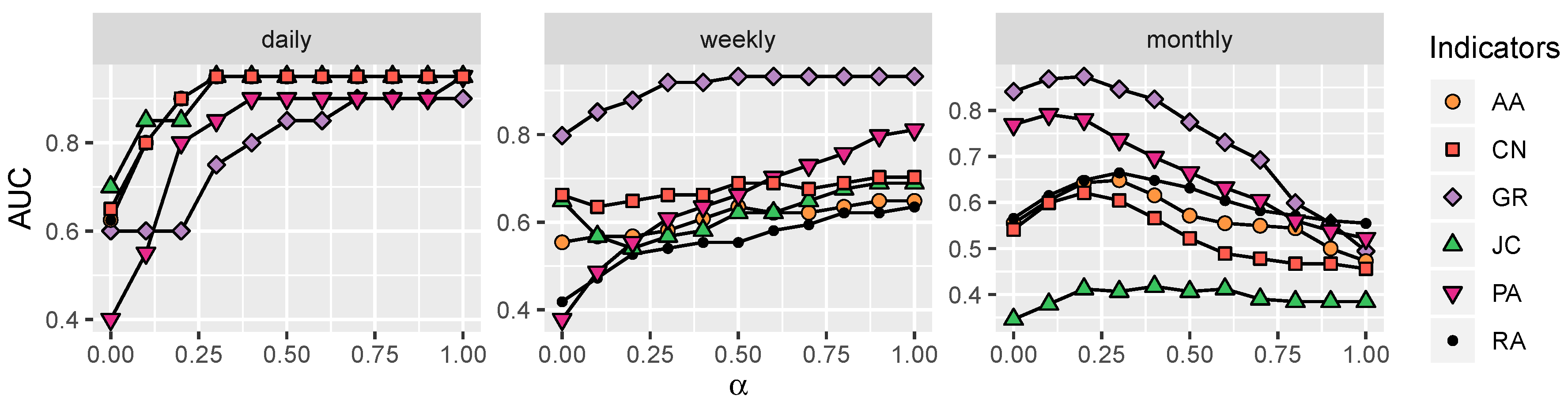
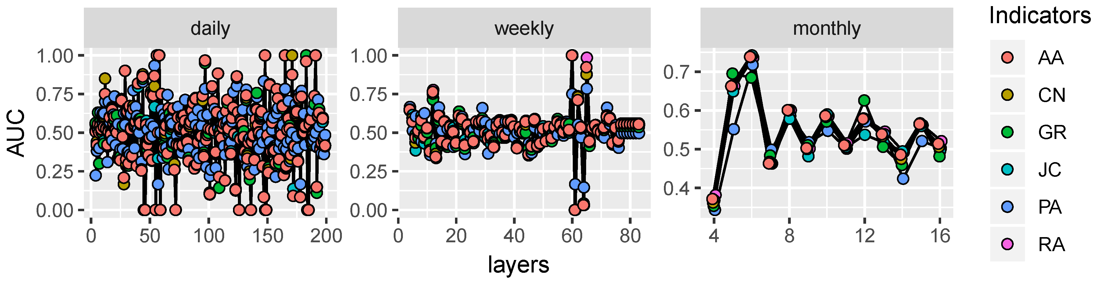
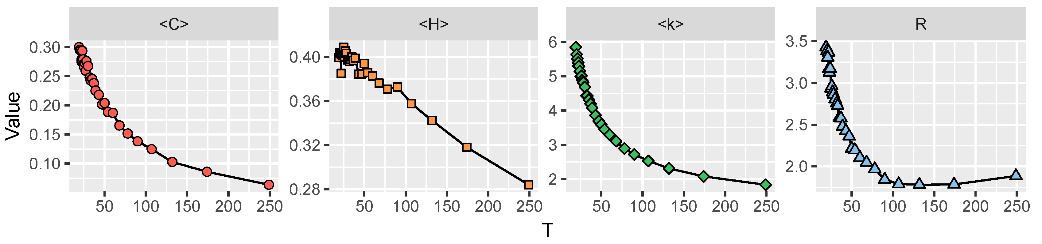
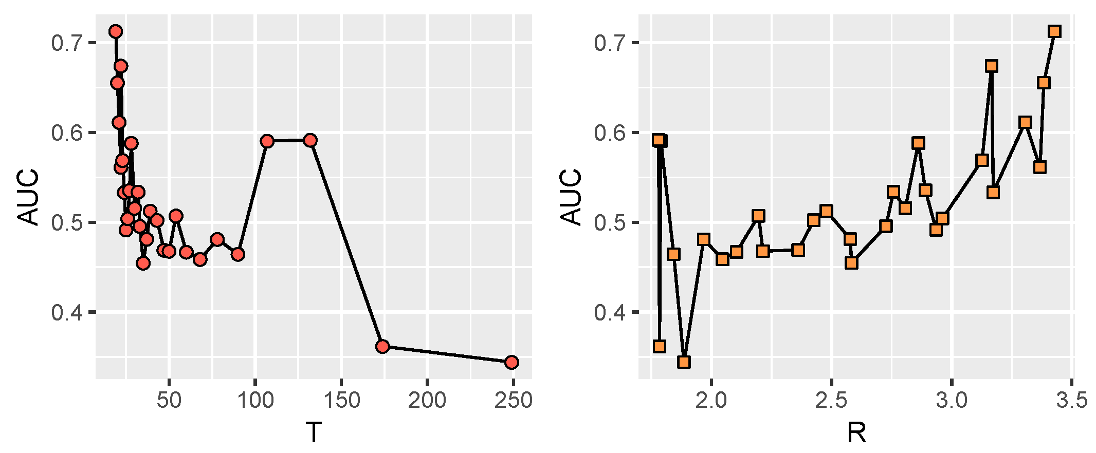
4.3. Parameters Analysis

In the proposed framework, parameters are crucial to the prediction results. Thus, in this subsection, the parameter $\alpha$ is analyzed and the results are plotted in Figure 6.

As shown in Figure 6, in a temporal network with a large number of slices, a larger $\alpha$ is preferred to be selected. On the contrary, when the temporal network is separated with fewer slices, a smaller $\alpha$ contributes to obtaining better performance. Finally, the robustness of the proposed method was verified by conducting experiments on different scales of temporal networks, as shown in Figure 7.

As shown in Figure 7, with the increasing of the number of slices (i.e., layers), the AUC result is changing periodically, and the varying range is stable generally. The results of the six indicators are in the same tendency, which verifies the robustness of the proposed method. To analyze the slicing effect on network features and performance, we conducted experiments with DS method and GR indicator. The results are shown in Figure 8 and Figure 9.

As shown in Figure 9 (left), the AUC result is declining as the number of slices increases. This results from the large numbers of intralayer edges of each time slice, which providing more edges to calculate the existence likelihood. Thus, we can utilize the network information more comprehensively. The performance is better with the ratio (i.e., intralayer edges comparing interlayer edges) increasing, as shown in Figure 9 (right).

5. Conclusions

Aiming at solving the problem of temporal links prediction in social networks, this paper proposes a novel dynamic similarity framework combining with an improved gravity model. Experiments on real-world datasets with different separations were conducted, and the experimental results show that the proposed method outperforms competitors. Afterwards, the determination of parameter $\alpha$ was analyzed by conducting a series of experiments, and we give the recommended selection for different temporal structures. Finally, the robustness of the proposed framework was also verified by comparing the obtained AUC results with varying time slices. Overall, the proposed framework is capable of predicting temporal links with reasonable results.

The contribution of this work is likely to benefit many real-world social applications, such as recommending new friends, protecting teenagers from harmful interactions, etc. Inspired by the multiple interactions among social actors, we have established a social platform, namely NEUSNCP (https://www.neusncp.com), for college students to make friends and share knowledge in various manners. By applying the proposed framework into recommending friends for newcomers, we have observed an obvious increase in user interactions. As part of future works, link prediction on more complicated models, i.e., multi-relational networks and bipartite networks on social platforms can be further studied. Notably, the research of recommendation for dynamic “user-blog” networks is in development, via a combination of collaborative filtering algorithm with temporal changes computation. In brief, the application of temporal links prediction is just unfolding.

References

1. Wasserman, S.; Faust, K. Social Network Analysis: Methods and Applications; Cambridge University Press: Cambridge, UK, 1994; Volume 8. [Google Scholar]
2. Antonacci, G.; Fronzetti Colladon, A.; Stefanini, A.; Gloor, P. It is rotating leaders who build the swarm: Social network determinants of growth for healthcare virtual communities of practice. J. Knowl. Manag. 2017, 21, 1218–1239. [Google Scholar] [CrossRef] [Green Version]
3. Sett, N.; Basu, S.; Nandi, S.; Singh, S.R. Temporal link prediction in multi-relational network. World Wide Web 2018, 21, 395–419. [Google Scholar] [CrossRef]
4. Getoor, L.; Diehl, C.P. Link mining: A survey. ACM SIGKDD Explor. Newslett. 2005, 7, 3–12. [Google Scholar] [CrossRef]
5. Srinivas, V.; Mitra, P. Link Prediction Using Thresholding Nodes Based on Their Degree. In Link Prediction in Social Networks; Springer: Berlin/Heidelberg, Germany, 2016; pp. 15–25. [Google Scholar]
6. Oyama, S.; Hayashi, K.; Kashima, H. Cross-temporal link prediction. In Proceedings of the 2011 IEEE 11th International Conference on Data Mining, Vancouver, BC, Canada, 11–14 December 2011; pp. 1188–1193. [Google Scholar]
7. Slokom, M.; Ayachi, R. A New Social Recommender System Based on Link Prediction Across Heterogeneous Networks. In Proceedings of the International Conference on Intelligent Decision Technologies, Sorrento, Italy, 17–19 June 2017; pp. 330–340. [Google Scholar]
8. Kim, W.; Kwon, K.; Kwon, S.; Lee, S. The identification power of smoothness assumptions in models with counterfactual outcomes. Quantit. Econ. 2018, 9, 617–642. [Google Scholar] [CrossRef]
9. Liben-Nowell, D.; Kleinberg, J. The link-prediction problem for social networks. J. Am. Soc. Inf. Sci. Technol. 2007, 58, 1019–1031. [Google Scholar] [CrossRef] [Green Version]
10. Lü, L.; Zhou, T. Link prediction in complex networks: A survey. Phys. A Stat. Mech. Appl. 2011, 390, 1150–1170. [Google Scholar] [CrossRef] [Green Version]
11. Pech, R.; Hao, D.; Pan, L.; Cheng, H.; Zhou, T. Link prediction via matrix completion. EPL (Europhys. Lett.) 2017, 117, 38002. [Google Scholar] [CrossRef] [Green Version]
12. Munasinghe, L.; Ichise, R. Time aware index for link prediction in social networks. In Proceedings of the International Conference on Data Warehousing and Knowledge Discovery, Toulouse, France, 29 August–2 September 2011; pp. 342–353. [Google Scholar]
13. Yasami, Y.; Safaei, F. A novel multilayer model for missing link prediction and future link forecasting in dynamic complex networks. Phys. A Stat. Mech. Appl. 2018, 492, 2166–2197. [Google Scholar] [CrossRef]
14. Kostakos, V. Temporal graphs. Phys. A Stat. Mech. Appl. 2009, 388, 1007–1023. [Google Scholar] [CrossRef] [Green Version]
15. Alhajj, R.; Rokne, J. Encyclopedia of Social Network Analysis and Mining; Springer: Berlin/Heidelberg, Germany, 2014. [Google Scholar]
16. Casteigts, A.; Flocchini, P.; Quattrociocchi, W.; Santoro, N. Time-varying graphs and dynamic networks. Int. J. Parallel Emerg. Distrib. Syst. 2012, 27, 387–408. [Google Scholar] [CrossRef]
17. Hua, T.D.; Nguyen-Thi, A.T.; Nguyen, T.A.H. Link prediction in weighted network based on reliable routes by machine learning approach. In Proceedings of the 2017 4th NAFOSTED Conference on Information and Computer Science, Hanoi, Vietnam, 24–25 November 2017; pp. 236–241. [Google Scholar]
18. Zhou, J.; Huang, D.; Wang, H. A dynamic logistic regression for network link prediction. Sci. China Math. 2017, 60, 165–176. [Google Scholar] [CrossRef]
19. Tabourier, L.; Bernardes, D.F.; Libert, A.S.; Lambiotte, R. RankMerging: A supervised learning-to-rank framework to predict links in large social networks. Mach. Learn. 2019, 108, 1729–1756. [Google Scholar] [CrossRef] [Green Version]
20. Hyndman, R.J.; Athanasopoulos, G. Forecasting: Principles and Practice; OTexts: Melbourne, Australia, 2018. [Google Scholar]
21. Hyndman, R.; Koehler, A.B.; Ord, J.K.; Snyder, R.D. Forecasting with Exponential Smoothing: The State Space Approach; Springer Science & Business Media: Berlin/Heidelberg, Germany, 2008. [Google Scholar]
22. Divakaran, A.; Mohan, A. Temporal Link Prediction: A Survey. New Gener. Comput. 2019. [Google Scholar] [CrossRef]
23. Özcan, A.; Öğüdücü, Ş.G. Multivariate temporal link prediction in evolving social networks. In Proceedings of the 2015 IEEE/ACIS 14th International Conference on Computer and Information Science (ICIS), Las Vegas, NV, USA, 28 June–1 July 2015; pp. 185–190. [Google Scholar]
24. Lorrain, F.; White, H.C. Structural equivalence of individuals in social networks. J. Math. Soc. 1971, 1, 49–80. [Google Scholar] [CrossRef]
25. Worth, D. Introduction to modern information retrieval. Aust. Acad. Res. Libr. 2010, 41, 305–306. [Google Scholar] [CrossRef] [Green Version]
26. Jaccard, P. Étude comparative de la distribution florale dans une portion des Alpes et des Jura. Bull. Soc. Vaudoise Sci. Nat. 1901, 37, 547–579. [Google Scholar]
27. Sorensen, T.A. A method of establishing groups of equal amplitude in plant sociology based on similarity of species content and its application to analyses of the vegetation on Danish commons. Biol. Skar. 1948, 5, 1–34. [Google Scholar]
28. Ravasz, E.; Somera, A.L.; Mongru, D.A.; Oltvai, Z.N.; Barabási, A.L. Hierarchical organization of modularity in metabolic networks. Science 2002, 297, 1551–1555. [Google Scholar] [CrossRef] [Green Version]
29. Molloy, M.; Reed, B. A critical point for random graphs with a given degree sequence. Random Struct. Algorithms 1995, 6, 161–180. [Google Scholar] [CrossRef]
30. Adamic, L.A.; Adar, E. Friends and neighbors on the web. Soc. Netw. 2003, 25, 211–230. [Google Scholar] [CrossRef] [Green Version]
31. Zhou, T.; Lü, L.; Zhang, Y.C. Predicting missing links via local information. Eur. Phys. J. B 2009, 71, 623–630. [Google Scholar] [CrossRef] [Green Version]
32. Barabási, A.L.; Albert, R. Emergence of scaling in random networks. Science 1999, 286, 509–512. [Google Scholar] [CrossRef] [PubMed] [Green Version]
33. Lü, L.; Jin, C.H.; Zhou, T. Similarity index based on local paths for link prediction of complex networks. Phys. Rev. E 2009, 80, 046122. [Google Scholar] [CrossRef] [PubMed] [Green Version]
34. Katz, L. A new status index derived from sociometric analysis. Psychometrika 1953, 18, 39–43. [Google Scholar] [CrossRef]
35. Leicht, E.A.; Holme, P.; Newman, M.E. Vertex similarity in networks. Phys. Rev. E 2006, 73, 026120. [Google Scholar] [CrossRef] [Green Version]
36. Liu, W.; Lü, L. Link prediction based on local random walk. EPL (Europhys. Lett.) 2010, 89, 58007. [Google Scholar] [CrossRef] [Green Version]
37. Vragović, I.; Louis, E. Network community structure and loop coefficient method. Phys. Rev. E 2006, 74, 016105. [Google Scholar] [CrossRef]
38. Klein, D.J.; Randić, M. Resistance distance. J. Math. Chem. 1993, 12, 81–95. [Google Scholar] [CrossRef]
39. Jeh, G.; Widom, J. SimRank: A measure of structural-context similarity. In Proceedings of the eighth ACM SIGKDD International Conference on Knowledge Discovery and Data Mining, Edmonton, AB, Canada, 23–26 July 2002; pp. 538–543. [Google Scholar]
40. Fouss, F.; Pirotte, A.; Renders, J.M.; Saerens, M. Random-walk computation of similarities between nodes of a graph with application to collaborative recommendation. IEEE Trans. Knowl. Data Eng. 2007, 19, 355–369. [Google Scholar] [CrossRef]
41. Sun, D.; Zhou, T.; Liu, J.G.; Liu, R.R.; Jia, C.X.; Wang, B.H. Information filtering based on transferring similarity. Phys. Rev. E 2009, 80, 017101. [Google Scholar] [CrossRef] [Green Version]
42. Chebotarev, P.Y.; Shamis, E. A matrix-forest theorem and measuring relations in small social group. Avtomatika i Telemekhanika 1997, 58, 125–137. [Google Scholar]
43. Boccaletti, S.; Bianconi, G.; Criado, R.; Del Genio, C.I.; Gómez-Gardenes, J.; Romance, M.; Sendina-Nadal, I.; Wang, Z.; Zanin, M. The structure and dynamics of multilayer networks. Phys. Rep. 2014, 544, 1–122. [Google Scholar] [CrossRef] [Green Version]
44. Paranjape, A.; Benson, A.R.; Leskovec, J. Motifs in temporal networks. In Proceedings of the Tenth ACM International Conference on Web Search and Data Mining, Cambridge, UK, 6–10 February 2017; pp. 601–610. [Google Scholar]
45. Fawcett, T. An introduction to ROC analysis. Pattern Recognit. Lett. 2006, 27, 861–874. [Google Scholar] [CrossRef]
46. Li, Z.; Ren, T.; Ma, X.; Liu, S.; Zhang, Y.; Zhou, T. Identifying influential spreaders by gravity model. Sci. Rep. 2019, 9, 8387. [Google Scholar] [CrossRef] [PubMed] [Green Version]
47. Chen, D.; Kong, L.; Wang, D.; Huang, X.; Fang, B. TNLCD: A Feasible Algorithm for Local Community Discovery in Temporal Networks. In FSDM; IOS Press: Amsterdam, The Netherlands, 2018; pp. 459–464. [Google Scholar]
48. Wang, P.; Xu, B.; Wu, Y.; Zhou, X. Link prediction in social networks: The state-of-the-art. Sci. China Inf. Sci. 2015, 58, 1–38. [Google Scholar] [CrossRef] [Green Version]
49. Zachary, W.W. An information flow model for conflict and fission in small groups. J. Anthropol. Res. 1977, 33, 452–473. [Google Scholar] [CrossRef] [Green Version]
50. Lusseau, D.; Schneider, K.; Boisseau, O.J.; Haase, P.; Slooten, E.; Dawson, S.M. The bottlenose dolphin community of Doubtful Sound features a large proportion of long-lasting associations. Behav. Ecol. Sociobiol. 2003, 54, 396–405. [Google Scholar] [CrossRef]
51. Tsvetovat, M.; Kouznetsov, A. Social Network Analysis for Startups: Finding Connections on the Social Web; O’Reilly Media, Inc.: Sebastopol, CA, USA, 2011. [Google Scholar]
52. Newman, M.E. Modularity and community structure in networks. Proc. Natl. Acad. Sci. USA 2006, 103, 8577–8582. [Google Scholar] [CrossRef] [Green Version]
53. Girvan, M.; Newman, M.E. Community structure in social and biological networks. Proc. Natl. Acad. Sci. USA 2002, 99, 7821–7826. [Google Scholar] [CrossRef] [Green Version]
54. Watts, D.J.; Strogatz, S.H. Collective dynamics of ‘small-world’ networks. Nature 1998, 393, 440. [Google Scholar] [CrossRef]
55. Hu, H.B.; Wang, X.F. Unified index to quantifying heterogeneity of complex networks. Phys. A Stat. Mech. Appl. 2008, 387, 3769–3780. [Google Scholar] [CrossRef]
Figure 1. Snapshot of temporal network of the first five days.
Symmetry 12 00100 g001
Figure 2. Supra-adjacency matrix representation. The diagonal blocks with different colors represent the network structures at different snapshots.
Symmetry 12 00100 g002
Figure 3. Illustration of τ function with different parameters. α varies in [0, 1], which depicts the attenuation level. The larger is α , the less effect there is on the current x.
Symmetry 12 00100 g003
Figure 4. Email-Eu-core-temporal-Dept3 network for link prediction in the dynamic network (daily, weekly, and monthly separated).
Symmetry 12 00100 g004
Figure 5. Comparison of temporal links prediction on Email-Eu-core-Dept3 network.
Symmetry 12 00100 g005
Figure 6. Analyzing parameter α in the temporal network with different separations. In general, the obtained AUC is larger with α increasing when the networks are daily and weekly separated.
Symmetry 12 00100 g006
Figure 7. Robustness verification by varying layers (or time slices).
Symmetry 12 00100 g007
Figure 8. Illustration of network features with varying numbers of slicing. T is the number of slices ranging from 17 to 249. <C>, <H>, and <k> are the average clustering coefficient [54], average heterogeneity [55], and average degree of the nodes in all slices, respectively. R is the ratio of intralayer edges comparing interlayer edges. In general, R declines when the temporal network is separated into more slices.
Symmetry 12 00100 g008
Figure 9. Relationship of performance with T (i.e., number of slices) and R (i.e., intralayer edges comparing interlayer edges). AUC declines with T increasing (or R declining) in general.
Symmetry 12 00100 g009