Axion Stars ^†

Abstract

The dark matter particle can be a QCD axion or axion-like particle. A locally over-densed distribution of axions can condense into a bound Bose–Einstein condensate called an axion star, which can be bound by self-gravity or bound by self-interactions. It is possible that a significant fraction of the dark matter axion is in the form of axion stars. This would make some efforts searching for the axion as the dark matter particle more challenging, but at the same time it would also open up new possibilities. Some of the properties of axion stars, including their emission rates and their interactions with other astrophysical objects, are not yet completely understood.

1. Introduction

The QCD axion is one of the best motivated dark matter particle candidates, since it provides a solution to the QCD strong $CP$ problem. (For a recent review, see [1].) The QCD axion is a boson with spin-0. It has a tiny mass and extremely weak couplings with the Standard Model particles, as well as extremely weak self-interactions. However, axion dark matter is not simple because axions are identical bosons. Its tiny mass indicates that if a large proportion of dark matter is axions, the occupation numbers can be very large. Therefore, the axions can form a Bose–Einstein condensate (BEC). The collective behavior of BEC can be very different from an ideal gas of bosons. The axion BEC can be bound gravitationally, which are called axion stars, or bound by self-interactions, which are called axitons. (For a recent review, see [2].) If a large fraction of the axion dark matter is in such bound configurations, the theoretical predictions of the behavior of dark matter could be dramatically different, which would affect the experimental searches.

The QCD axion has been strongly constrained [1]. The allowed range of axion mass has been reduced to between ${10}^{-6}$ and ${10}^{-2}$ eV. Axion dark matter can also more generally refer to other light spin-0 boson with a periodic potential for self-interaction. There are motivations from string theory and astrophysics for a dark matter particle that is a very light boson with mass as light as ${10}^{-22}$ eV [3,4,5]. In this proceeding, we focus mainly on the QCD axion, but many of our results are presented in a form that can be applied to other axion-like particles straightforwardly.

2. Axion Field Theories at Different Energy Scales

The fundamental quantum field theory for the QCD axion is an extension of the Standard Model with Peccei–Quinn (PQ) $U\left(1\right)$ symmetry. PQ symmetry is spontaneously broken by the ground state of a complex Lorentz–scalar field [6,7,8]. After symmetry breaking, the minima of the potential are a circle of radius $f_a$, which is called the axion decay constant. At momentum scales of order $f_a$, the axion field is the Goldstone mode corresponding to excitation of the scalar field along that circle.

The axion can be described by a field theory with a real Lorentz–scalar field $\varphi \left(x\right)$ at momentum scales much smaller than $f_a$. Its potential must have the shift symmetry with $\varphi \left(x\right)=\varphi \left(x\right)+2\pi f_a$. When the energy scale is below the week scale, which is about 100 GeV, the interactions between axions and the Standard Model particles are:

$$\frac{{\alpha }_s}{8\pi f_a}\varphi G_{\mu \nu }^a{\tilde{G}}^{a\mu \nu }+\frac{c_{\gamma 0}\alpha }{8\pi f_a}\varphi F_{\mu \nu }{\tilde{F}}^{\mu \nu }+\frac{1}{2f_a}{J}^{\mu }{\partial }_{\mu }\varphi ,$$

(1)

where $G_{\mu \nu }^a$ and $F_{\mu \nu }$ are the QCD and QED field strengths, ${\tilde{G}}_{\mu \nu }^a=\frac{1}{2}{ϵ}_{\mu \nu \lambda \sigma }{G}^{a\lambda \sigma }$ and ${\tilde{F}}_{\mu \nu }$ are the corresponding dual field strengths, and the current $J^{\mu }$ is a linear combination of axial-vector fermion currents. The specific value of $c_{\gamma 0}$ and the form of $J^{\mu }$ depend on the specific axion model. The QCD field-strength term in Equation (1) is proportional to the topological charge density ${\alpha }_s{G}_{\mu \nu }^a{\tilde{G}}^{a\mu \nu }/8\pi$. The shift symmetry of $\varphi$ is guaranteed by the quantization of the QCD topological charge in Euclidean field theory.

When the momentum scale is further below the scale of QCD confinement, which is about 1 GeV, the gluon degree of freedom is replaced by the degree of freedoms of hadrons. Then, the axion self-interactions from the coupling to the gluon field in Equation (1) can be described by a real potential $V\left(\varphi \right)$:

$$\mathcal{L}=\frac{1}{2}{\partial }_{\mu }\varphi {\partial }^{\mu }\varphi -V\left(\varphi \right).$$

(2)

The invariance of the Lagrangian under the shift symmetry $\varphi \left(x\right)\to \varphi \left(x\right)+2\pi f_a$ requires the potential $V\left(\varphi \right)$ to be a periodic function of $\varphi$: $V\left(\varphi \right)=V(\varphi +2\pi f_a)$. The Lagrangian is also invariant under the $Z_2$ symmetry $\varphi \left(x\right)\to -\varphi \left(x\right)$, which requires $V\left(\varphi \right)$ to be an even function of $\varphi$.

The potential $V\left(\varphi \right)$ for the axion field is determined by nonperturbative effects of QCD. The specific form can be systematically derived order-by-order from the chiral effective field theory for light pseudoscalar mesons of QCD and the axion [9]. The leading order potential derived from the chiral effective field theory for the axion and pions gives the chiral potential [10]:

$$V\left(\varphi \right)={\left(m_{\pi }{f}_{\pi }\right)}^2\left(1-\frac{\sqrt{1+z^2+2zcos(\varphi /f_a)}}{1+z}\right),$$

(3)

where $z=m_u/m_d$ is the ratio of the up quark and down quark masses. The coefficient can be calculated by the pion mass $m_{\pi }=135.0$ MeV and the pion decay constant $f_{\pi }=92.2$ MeV, which are related to $m_a$ and $f_a$ by [11]

$$m_{\pi }{f}_{\pi }=\frac{1+z}{\sqrt{z}}{m}_a{f}_a.$$

(4)

A next-to-leading order analysis in the chiral effective field theory gives the numerical value $z=0.48\left(3\right)$ [9]. With the upper and lower bounds on $f_a$ from cosmology and astrophysics, the allowed mass range for the QCD axion is between $6\times {10}^{-6}$ and $2\times {10}^{-3}$ eV [1]. In this proceeding, every time we provide a numerical value which depends on $m_a$, we give the value in the form:

$$m_a={10}^{-4\pm 1}\mathrm{eV}.$$

(5)

It should be understood, as the value is between ${10}^{-5}$ and ${10}^{-3}$ depending on the choice of the axion mass. In addition to the more precise chiral potential, a popular model for the axion potential that has been widely used in phenomenological studies is called the instanton potential:

$$V\left(\varphi \right)={\left(m_a{f}_a\right)}^2\left[1-cos(\varphi /f_a)\right].$$

(6)

It can be derived with a dilute instanton gas approximation [12], which cannot be improved systematically. The field theory given by the Lagrangian in Equation (2) with the instanton potential in Equation (6) is often called the sine-Gordon model.

The axion field can be more simply expressed as a complex scalar field in a nonrelativistic effective field theory (NREFT) when the energy scale is much smaller than the axion mass $m_a$. A naive way of deriving the NREFT is to replace the real field by the complex field $\psi$ with:

$$\varphi (\mathit{r},t)\approx \frac{1}{\sqrt{2m_a}}\left(\psi (\mathit{r},t)e^{-i{m}_{a}t}+{\psi }^{*}(\mathit{r},t)e^{+i{m}_{a}t}\right).$$

(7)

Then, by dropping out the terms with a rapidly oscillating phase in the form of $exp\left(in{m}_{a}t\right)$ with nonzero integer n, we can get the NREFT Lagrangian:

$${\mathcal{L}}_{\mathrm{eff}}=\frac{1}{2}i\left({\psi }^{*}\dot{\psi }-{\dot{\psi }}^{*}\psi \right)-{\mathcal{H}}_{\mathrm{eff}}.$$

(8)

This effective Hamiltonian density depends on the field $\psi$ and its gradients. It can be separated into three parts: ${\mathcal{H}}_{\mathrm{eff}}={\mathcal{T}}_{\mathrm{eff}}+V_{\mathrm{eff}}+W_{\mathrm{eff}}$, where ${\mathcal{T}}_{\mathrm{eff}}$ is the kinetic energy density, $V_{\mathrm{eff}}$ is a function of ${\psi }^{*}\psi$ only, and $W_{\mathrm{eff}}$ consists of all other interaction terms that also depend on gradients of $\psi$. An n-body term in ${\mathcal{H}}_{\mathrm{eff}}$ has n factors of $\psi$ and n factors of ${\psi }^{*}$, with arbitrary numbers of gradients. The kinetic energy density ${\mathcal{T}}_{\mathrm{eff}}$ includes all the one-body terms:

$${\mathcal{T}}_{\mathrm{eff}}=\frac{1}{2m_a}\nabla {\psi }^{*}·\nabla \psi -\frac{1}{8m_a^3}{\nabla }^2{\psi }^{*}{\nabla }^2\psi +\dots .$$

(9)

These terms reproduce the energy–momentum relation $E=\sqrt{m^2+p^2}-m$ in the nonrelativistic limit. The effective potential $V_{\mathrm{eff}}$ can be expanded in powers of ${\psi }^{*}\psi$ beginning at order ${\left({\psi }^{*}\psi \right)}^2$:

$$V_{\mathrm{eff}}\left({\psi }^{*}\psi \right)=m_a^2{f}_a^2\sum _{n=2}^{\infty }\frac{v_n}{{(n!)}^2}{\left(\frac{{\psi }^{*}\psi }{2m_a{f}_a^2}\right)}^n.$$

(10)

This NREFT Lagrangian can also be derived strictly by a nonlocal canonical transformation from the relativistic real scalar Lagrangian in Equation (2) [13]. The coefficients $v_n$ are complex numbers in general, which can be calculated by matching the scattering amplitudes at low energy [14,15,16]. The contributions from Feynman diagrams without an internal propogator can be summed into a compact form, which is:

$$\begin{array}{ccc}\hfill V_{\mathrm{eff}}^{\left(0\right)}\left({\psi }^{*}\psi \right)& =& {\left(m_{\pi }{f}_{\pi }\right)}^2\left(1-\frac{z}{4{(1+z)}^2}\widehat{n}-\frac{1}{1+z}{\int }_0^{1}dt\sqrt{1+z^2+2zcos({\widehat{n}}^{1/2}sin\left(\pi t\right))}\right),\hfill \end{array}$$

(11)

for chiral potential, and:

$$V_{\mathrm{eff}}^{\left(0\right)}\left({\psi }^{*}\psi \right)={\left(m_a{f}_a\right)}^2\left[1-\frac{1}{4}\widehat{n}-J_0\left({\widehat{n}}^{1/2}\right)\right].$$

(12)

for instanton potential, where $\widehat{n}=2{\psi }^{*}\psi /\left(m_a{f}_a^2\right)$ is the dimensionless number density. A systematic scheme of including the off-shell internal propagators is suggested in [14].

3. Axion Stars

3.1. Dilute Axion Stars

An axion star is a boson star made of axions. The boson star with bosons in BEC was first considered by Tkachev [17]. The classical solutions for a boson star can be obtained by solving the Einstein–Klein–Gordon equations for a real scalar field $\varphi (\mathit{r},t)$ with axion potential $V\left(\varphi \right)$. The solutions are approximately localized and periodic.

Stable solutions exist with the energy density at the center much lower than the QCD scale. We call these solutions dilute axion stars. The solutions of dilute axion stars can also be obtained using the axion NREFT with Newtonian gravity. The latter is much simpler and without loss of much accuracy:

$$\begin{array}{ccc}\hfill i\dot{\psi }& =& -\frac{1}{2m_a}{\nabla }^2\psi +\left[V_{\mathrm{eff}}^{\prime }\left({\psi }^{*}\psi \right)+m_a\Phi \right]\psi ,\hfill \end{array}$$

(13a)

$$\begin{array}{ccc}\hfill {\nabla }^2\Phi & =& 4\pi G{m}_a{\psi }^{*}\psi .\hfill \end{array}$$

(13b)

These equations are also called Gross–Pitaevskii–Poisson (GPP) equations. The number density ${\psi }^{*}\psi$ is much smaller compared to $m_a{f}_a^2$ for dilute axion stars. Thus, we can expand the effective potential and keep only the leading term:

$$V_{\mathrm{eff}}\left({\psi }^{*}\psi \right)\approx \frac{v_2}{16f_a^2}{\left({\psi }^{*}\psi \right)}^2.$$

(14)

Chavanis used the GPP equations with this leading term of the potential to derive simple approximations of the basic properties of boson stars with negative $v_2$ [18]. His results show that there is a maximum mass for the dilute axion stars $G^{-1/2}{f}_a/m_a$.

Variational methods has been used to get simple approximations to the dilute axion stars [18,19,20]. One can also match asymptotic expansions to get more accurate solutions [21]. the numerical method gives the most accurate solutions. The results below were obtained by numerically solving the GPP equations in Equation (13). The potential $V_{\mathrm{eff}}$ is either the naive effective instanton potential in Equation (12) or the naive effective chiral potential in Equation (11) with $z=0.48$.

In Figure 1, we show the dependence of the radius $R_{99}$ of the dilute axion star on the mass M. The critical point (indicated by the solid dot) separates the stable branch from the unstable branch. When the number density at the center $n_0$ increases, the solution moves from the left to the critical point along the stable branch. The dilute axion star at the critical point has the largest mass. Then, as $n_0$ keeps increasing, the solution moves from the critical point to the left along the unstable branch. The self-interaction of axions can be ignored for the stable solutions with a mass which is much smaller than the maximum mass. The self-interaction only plays an important role close to the critical point.

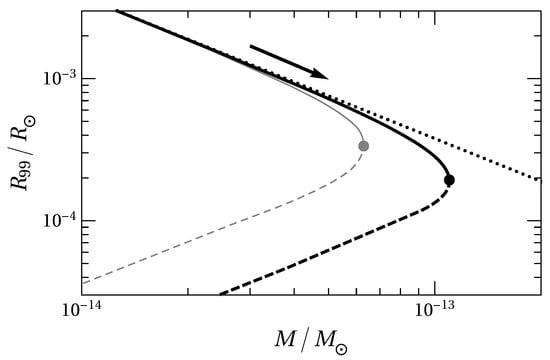
Figure 1. Radius $R_{99}$ versus mass M for dilute axion stars. The axion mass is $m_a={10}^{-4}$ eV. The curves are calculated with chiral potential with $z=0.48$ (black curves) or the instanton potential (gray curves). The dots are critical points at which the dilute axion stars have the maximum masses. The dots separate the unstable branch (dashed curve) from the stable branch (solid curve). For comparison, the boson stars with no self-interaction are shown with a dotted line. The arrow indicates the increase of axion star mass from the condensation of additional axions in the surroundings.

The properties of the critical point in Figure 1 are important in phenomenology. The number of axions in the dilute axion star with the chiral potential with $z=0.48$ is $N_{*}=1.2\times {10}^{57\mp 3}$ for axion mass $m_a={10}^{-4\pm 1}$ eV. (This number is smaller by the factor 0.59 for instanton potential because of the different value of $v_2$.) The corresponding critical dilute axion star is $N_{*}{m}_a=1.1\times {10}^{-13\mp 4}{M}_{\odot }$, with $M_{\odot }$ as the mass of the Sun. The critical radius $R_{99*}=1.9\times {10}^{-4}{R}_{\odot }$, with $R_{\odot }$ as the radius of the Sun. More properties of the dilute axion stars can be found in [2].

3.2. Dense Axion Stars

In [22], we pointed out that there could be other stable branches of axion star solutions with larger center density. Another branch can be found by following the unstable solution from the critical dilute axion stars in Figure 1. With a larger center density, at some point, we need to consider all terms in the expansion of the potential $V_{\mathrm{eff}}\left({\psi }^{*}\psi \right)$. In [22], we solved the field equation in Equation (13) with the naive effective instanton potential in Equation (12). In [2], the results using the naive effective chiral potential in Equation (11) are obtained, which are also shown in Figure 2. A second critical point was found with the radius smaller by 7 orders of magnitude. The localized solutions near and beyond the second critical point were called the dense axion stars in [22], because the mass density $m_a{\psi }^{*}\psi$ at the center of the axion star becomes comparable to the QCD scale ${\left(m_a{f}_a\right)}^2$.

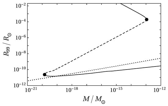
Figure 2. Radius $R_{99}$ versus mass M for axion stars. The solutions are obtained with $m_a={10}^{-4}$ eV and the naive chiral potential with $z=0.48$. The stable branches (solid curves) and unstable branch (dashed curves) are separated by critical points (labeled with black dots). The upper-left critical point is the same as the black dot in Figure 1. A second critical point is found by following the unstable solution to larger center density. Also shown is the Thomas–Fermi approximation (dotted curve).

For the dense axion stars near the second critical point in Figure 2, the contribution of gravity is almost negligible. Thus, the dense axion stars near the second critical point are actually oscillons. The oscillons are approximately localized solutions of a real scalar field, which are bound only by self-interactions. For the chiral potential with $m_a={10}^{-4\pm 1}$ eV and $z=0.48$, the critical number of axions is $N_{*}=2\times {10}^{50\mp 4}$. The critical mass $N_{*}{m}_a$ is $3\times {10}^{10\mp 3}$ kg, and the critical radius $R_{99*}$ is $2\times {10}^{-2\mp 1}$ m. More properties of the critical dense axion stars can be found in [2].

As shown in Figure 2, beyond the lower critical point, the mass M of the dense axion star increases as a function of the radius $R_{99}$. With larger central density, the dense axion star curve approaches the Thomas–Fermi approximation [23], which is the straight dotted line in Figure 2. In the Thomas–Fermi approximation, the kinetic pressure is ignored except on the surface of the stars; in the bulk, it is the repulsive force from axion self-interaction which balances the attractive force from gravity. In [22], the Thomas–Fermi approximation was mistakenly used to extrapolate the curve of $R_{99}$ to very large values of M. As pointed out in [24], the curve for $R_{99}$ versus M actually crosses the line of the Thomas–Fermi approximation at a small angle. Therefore, the Thomas–Fermi approximation is not a proper estimate for dense axion stars.

4. Theoretical Issues

Below, we have listed two prominent theoretical issues on axion stars. More details can be found in [2].

4.1. Emission from Axion Stars

As the axion is a real scalar field, the number of axions is not conserved. Self-interactions can convert the nonrelativistic axions into relativisitic ones. The axion stars and any other localized axion configuration with nonrelativisitic axions, inevitably radiate axion waves with relativistic wavelengths. As a result, the axion stars have finite lifetimes. It is important to calculate the lifetime of axion stars, since it determines whether they can have any observational significance.

NREFT appears to give unambiguous predictions for the conversion rate of nonrelativistic axions in axion stars into outgoing relativisitic axion waves [15]. The rate of decrease in N, the total number of nonrelativistic axions, is described by the anti-Hermitian terms in the effective Hamiltonian. When the number density of axions is small, such as in a dilute axion star, the loss of nonrelativistic axions is dominated by the decay into two photons. Thus the decay rate of the dilute axion star is the same as the decay rate of a single axion. The lifetime of a dilute axion star is therefore much longer than the age of the universe. For dense configurations, we define the lifetime to be the time required for the total number of axions to decrease by a factor $1/e$, when it moves to the left along the lower branch in Figure 2. In a dense axion star, the loss rate from the $4\to 2$ process is approximately 5 orders of magnitude larger than that from $a\to 2\gamma$. The resulting predictions for the lifetime of the dense axion stars are still much longer than the age of the universe [15].

The predictions of NREFT for the loss rate of nonrelativistic axions are, however, incomplete. Surprisingly, there are loss processes for axions in the relativistic theory that cannot be reproduced by NREFT. NREFT is expect to correctly reproduce results from the corresponding relativistic theory for an oscillon with a small boson binding energy ${\epsilon }_b\ll m_a$ as an expansion in powers of ${\epsilon }_b/m_a$. However, such an expansion is blind to terms which are exponentially small in $m_a/{\epsilon }_b$, such as $exp(-c\sqrt{m_b/{\epsilon }_b})$, where c is some constant. Thus, we should not expect a contribution having such an exponential factor to be reproduced by NREFT.

The contribution of loss processes whose rates have exponentially small factors can be calculated from the asymptotic expansion for the oscillon [25]. These terms have a radiative tail in the form of standing waves with exponentially small amplitudes that extend to infinity and have infinite energy. Without incoming waves, the outgoing waves decrease the total number of nonrelativistic axions of the localized part of the solution. The rate of decrease in the particle number, or equivalently the mass M, of the oscillon with angular frequency $\omega =\sqrt{1-{ϵ}^2}{m}_a$ in the limit $ϵ\to 0$ has the form [26]:

$$-\frac{dM}{dt}=\frac{A}{{ϵ}^2}exp(-3.406/ϵ)f_a^2,$$

(15)

where the prefactor A depends on the axion potential $V\left(\varphi \right)$. The sine-Gordon model is a special case in which A is suppressed by ${ϵ}^2$. For the sine-Gordon model in 3D, A is calculated to be $760.5{ϵ}^2$ [26].

Eby et al. derived an expression for the loss rate that can be expressed in terms of the complex field $\psi \left(x\right)$ of NREFT [27]. Their derivation involves the matrix element of $V\left(\varphi \right)$ inserted between an initial state of N condensed axions, each with energy $\omega =m_a-{\epsilon }_b$, and a final state consisting of $N-3$ condensed axions plus an on-shell relativistic axion with energy $3\omega$. This can be interpreted as a $3\to 1$ interaction, which is forbidden in the vacuum by conservation of momentum and energy. Their result for the rate of energy loss [27] can be expressed in the form:

$$-\frac{dM}{dt}=\frac{m_a\omega k}{192\pi f_a^4}{\left|\int d^{3}r{e}^{i\mathit{k}·\mathit{r}}\left[{\lambda }_4+\frac{{\lambda }_6{\psi }^{*}\psi }{8m_a{f}_a^2}+\dots \right]{\psi }^3\right|}^2,$$

(16)

where ${\mathit{k}}^2=9{\omega }^2-m_a^2$ and $\psi \left(r\right)$ is the wavefunction of the condensed axions normalized so the number of axions is $\int d^{3}r{\psi }^{*}\psi$. A result consistent with Equation (16) was also obtained in [28], where this loss mechanism was referred to as “decay via spatial gradients”. Since $\left|\mathit{k}\right|\approx \sqrt{8}{m}_a$, the loss comes from the small high-momentum tail of the wavefunction. For the instanton potential, its expansion in powers of ${\psi }^{*}\psi$ in Equation (16) can be summed up to all orders in terms of a Bessel function [27]. Eby et al. obtained a result for the loss rate in Equation (16) for the sine-Gordon model in the limit ${\epsilon }_b\to 0$ [29]. Their exponential suppression factor is consistent with Equation (15), but with the argument differing by less than 2%. Moreover, their result for the coefficient in the prefactor is $A=2723$. It is different from the result in [26] by lacking a suppression factor of ${ϵ}^2$.

4.2. Collapse of Dilute Axion Stars

If a dilute axion star is embedded in a gas of unbounded axions, thermalization can condense additional axions and increase the mass of the axion star. For dilute axion stars close to the critical mass $M_{*}\approx N_{*}{m}_a$, where $N_{*}$ is the total number of axions in the star, further condensation of axions can increase M to above $M_{*}$. Then, it will be unstable and collapse. The remnant of a collapsing dilute axion star has not been understood definitely. The possibilities for the remnant after the collapse include:

• A black hole, with a Schwarzschild radius which is smaller than the critical radius $R_{99*}$ by about 15 orders of magnitude;
• A dense axion star, with a radius which is smaller than $R_{99*}$ by about 7 orders of magnitude;
• A dilute axion star, with a radius which is larger than $R_{99*}$; and
• No remnant, because of complete disappearance into scalar waves.

Chavanis considered the possibility that a collapsing dilute axion star produces a black hole in [30]. The evolution of the axion field is obtained by solving the GPP equations for $\psi$ and $\Phi$ given by Equation (13) with the truncated effective potential $V_{\mathrm{eff}}$ in Equation (14). He assumes the configuration for the complex axion field $\psi (r,t)$ can always be described by a Gaussian function, with a time-dependent radius $R\left(t\right)$. He found the time for collapse to $R=0$ scales as ${(M-M_{*})}^{-1/4}$ if the initial configuration is an unstable solution with mass M near $M_{*}$. Same variational methods were used previously to study the time evolution of gravitationally bound BECs of bosons with a positive scattering length [31].

Eby et al. also studied the collapse of dilute axion stars using a similar time-dependent variational approximation, but with $V_{\mathrm{eff}}$ given by the naive instanton effective potential in Equation (12) [32,33]. They found that the collapsing process is hindered by repulsive terms in the effective potential, which becomes important when the radius is close to that of a dense axion star. A large fraction of the total number of axions is lost through the emission of relativistic axions. But they were unable to determine definitely whether the remnant is a dense axion star.

Helfer et al. studied the fate of spherically symmetric axion configurations by solving the full nonlinear classical field equations in the framework of general relativity for axions with the instanton potential [34]. After evolving the configurations in time, they found the remnant could be a black hole or a dilute axion star or that there could be no remnant. Their calculations were limited to the parameter region $4\times {10}^{-8}<G{f}_a^2<4\times {10}^{-2}$ and $0.03<GM{m}_a<0.12$. The three different possibilities for the remnant depend on different regions of the plane of $G{f}_a^2$ versus $GM{m}_a$. The three regions meet at a triple point given by $G{f}_a^2=3.6\times {10}^{-3}$ and $GM{m}_a=0.095$. By extrapolating the results of [34] to the tiny value of $G{f}_a^2$ for the QCD axion, one finds that the possibilities could be a black hole or no remnant.

Levkov, Panin, and Tkachev numerically calculated the collapse of dilute axion stars above the critical mass with the GPP equations [35]. Their solutions approach a self-similar scaling limit with a series of singularities at finite times $t_{*}$. Their calculation shows multiple cycles of growth of the energy density close to the center of the star followed by collapsing. The collapse dramatically increases the energy density near the center, followed by a burst of outgoing relativistic axion waves, which effectively depletes the energy density near the center. Levkov et al. also found that after these multiple cycles, the remnant is still gravitationally bound. They therefore concluded that the remnant must ultimately relax to a less-massive dilute axion star by gravitational cooling.

References

- Kim, J.E.; Carosi, G. Axions and the strong CP problem. Rev. Mod. Phys. 2010, 82, 557. [Google Scholar] [CrossRef]
- Braaten, E.; Zhang, H. Colloquium: The physics of axion stars. Rev. Mod. Phys. 2019, 91, 41002. [Google Scholar] [CrossRef]
- Arvanitaki, A.; Dimopoulos, S.; Dubovsky, S.; Kaloper, N.; March-Russell, J. String axiverse. Phys. Rev. D 2010, 81, 123530. [Google Scholar] [CrossRef]
- Hu, W.; Barkana, R.; Gruzinov, A. Fuzzy cold dark matter: the wave properties of ultralight particles. Phys. Rev. Lett. 2000, 85, 1158. [Google Scholar] [CrossRef] [PubMed]
- Hui, L.; Ostriker, J.P.; Tremaine, S.; Witten, E. Ultralight scalars as cosmological dark matter. Phys. Rev. D 2017, 95, 43541. [Google Scholar] [CrossRef]
- Peccei, R.D.; Quinn, H.R. CP Conservation in the Presence of Instantons. Phys. Rev. Lett. 1977, 38, 1440. [Google Scholar] [CrossRef]
- Weinberg, S. A new light boson? Phys. Rev. Lett. 1978, 40, 223. [Google Scholar] [CrossRef]
- Wilczek, F. Problem of strong P and T invariance in the presence of instantons. Phys. Rev. Lett. 1978, 40, 279. [Google Scholar] [CrossRef]
- di Cortona, G.G.; Hardy, E.; Vega, J.P.; Villadoro, G. The QCD axion, precisely. JHEP 2016, 1601, 34. [Google Scholar] [CrossRef]
- di Vecchia, P.; Veneziano, G. Chiral dynamics in the large N limit. Nucl. Phys. B 1980, 171, 253. [Google Scholar] [CrossRef]
- Bardeen, W.A.; Tye, S.-H.H. Current algebra applied to properties of the light Higgs boson. Phys. Lett. B 1978, 74, 229. [Google Scholar] [CrossRef]
- Peccei, R.D.; Quinn, H.R. Constraints imposed by CP conservation in the presence of pseudoparticles. Phys. Rev. D 1977, 16, 1791. [Google Scholar] [CrossRef]
- Namjoo, M.H.; Guth, A.H.; Kaiser, D.I. Relativistic corrections to nonrelativistic effective field theories. Phys. Rev. D 2018, 98, 16011. [Google Scholar] [CrossRef]
- Braaten, E.; Mohapatra, A.; Zhang, H. Nonrelativistic effective field theory for axions. Phys. Rev. D 2016, 94, 76004. [Google Scholar] [CrossRef]
- Braaten, E.; Mohapatra, A.; Zhang, H. Emission of photons and relativistic axions from axion stars. Phys. Rev. D 2017, 96, 31901. [Google Scholar] [CrossRef]
- Braaten, E.; Mohapatra, A.; Zhang, H. Classical nonrelativistic effective field theories for a real scalar field. Phys. Rev. D 2018, 98, 96012. [Google Scholar] [CrossRef]
- Tkachev, I.I. On the possibility of Bose star formation. Phys. Lett. B 1991, 261, 289. [Google Scholar] [CrossRef]
- Chavanis, P.H. Mass-radius relation of Newtonian self-gravitating Bose-Einstein condensates with short-range interactions: I. Analytical results. Phys. Rev. D 2011, 84, 43531. [Google Scholar] [CrossRef]
- Schiappacasse, E.D.; Hertzberg, M.P. Analysis of dark matter axion clumps with spherical symmetry. JCAP 2018, 1801, 37, Erratum in 2018, 1803, E01. [Google Scholar] [CrossRef]
- Eby, J.; Leembruggen, M.; Street, L.; Suranyi, P.; Wijewardhana, L.C.R. Approximation methods in the study of boson stars. Phys. Rev. D 2018, 98, 123013. [Google Scholar] [CrossRef]
- Kling, F.; Rajaraman, A. Profiles of boson stars with self-interactions. Phys. Rev. D 2018, 97, 63012. [Google Scholar] [CrossRef]
- Braaten, E.; Mohapatra, A.; Zhang, H. Dense Axion Stars. Phys. Rev. Lett. 2016, 117, 121801. [Google Scholar] [CrossRef] [PubMed]
- Wang, X.Z. Cold Bose stars: Self-gravitating Bose-Einstein condensates. Phys. Rev. D 2001, 64, 124009. [Google Scholar] [CrossRef]
- Visinelli, L.; Baum, S.; Redondo, J.; Freese, K.; Wilczek, F. Dilute and dense axion stars. Phys. Lett. B 2018, 777, 64. [Google Scholar] [CrossRef]
- Segur, H.; Kruskal, M.D. Nonexistence of small amplitude breather solutions in ϕ4 theory. Phys. Rev. Lett. 1987, 58, 747. [Google Scholar] [CrossRef] [PubMed]
- Fodor, G.; Forgacs, P.; Horvath, Z.; Mezei, M. Radiation of scalar oscillons in 2 and 3 dimensions. Phys. Lett. B 2009, 674, 319. [Google Scholar] [CrossRef]
- Eby, J.; Suranyi, P.; Wijewardhana, L.C.R. The lifetime of axion stars. Mod. Phys. Lett. A 2016, 31, 1650090. [Google Scholar] [CrossRef]
- Mukaida, K.; Takimoto, M.; Yamada, M. On longevity of I-ball/oscillon. JHEP 2017, 1703, 122. [Google Scholar] [CrossRef]
- Eby, J.; Ma, M.; Suranyi, P.; Wijewardhana, L.C.R. Decay of ultralight axion condensates. JHEP 2018, 1801. [Google Scholar] [CrossRef]
- Chavanis, P.H. Collapse of a self-gravitating Bose-Einstein condensate with attractive self-interaction. Phys. Rev. D 2016, 94, 83007. [Google Scholar] [CrossRef]
- Harko, T. Gravitational collapse of Bose-Einstein condensate dark matter halos. Phys. Rev. D 2014, 89, 84040. [Google Scholar] [CrossRef]
- Eby, J.; Leembruggen, M.; Suranyi, P.; Wijewardhana, L.C.R. Collapse of axion stars. JHEP 2016, 1612. [Google Scholar] [CrossRef]
- Eby, J.; Leembruggen, M.; Suranyi, P.; Wijewardhana, L.C.R. QCD axion star collapse with the chiral potential. JHEP 2017, 1706, 14. [Google Scholar] [CrossRef]
- Helfer, T.; Marsh, D.J.E.; Clough, K.; Fairbairn, M.; Lim, E.A.; Becerril, R. Black hole formation from axion stars. JCAP 2017, 1703, 55. [Google Scholar] [CrossRef]
- Levkov, D.G.; Panin, A.G.; Tkachev, I.I. Relativistic axions from collapsing Bose stars. Phys. Rev. Lett. 2017, 118, 11301. [Google Scholar] [CrossRef] [PubMed]
© 2019 by the author. Licensee MDPI, Basel, Switzerland. This article is an open access article distributed under the terms and conditions of the Creative Commons Attribution (CC BY) license (http://creativecommons.org/licenses/by/4.0/).