Article

A Method of L1-Norm Principal Component Analysis for Functional Data

1
School of Statistics, Capital University of Economics and Business, Beijing 100071, China
2
School of Science, Chongqing University of Posts and Telecommunications, Chongqing 400065, China
3
School of Computer Science and Technology, Chongqing University of Posts and Telecommunications, Chongqing 400065, China
*
Author to whom correspondence should be addressed.
Symmetry 2020, 12(1), 182; https://doi.org/10.3390/sym12010182
Submission received: 15 December 2019 / Revised: 5 January 2020 / Accepted: 10 January 2020 / Published: 20 January 2020
(This article belongs to the Special Issue Novel Machine Learning Approaches for Intelligent Big Data 2019)

Abstract

:
Recently, with the popularization of intelligent terminals, research on intelligent big data has been paid more attention. Among these data, a kind of intelligent big data with functional characteristics, which is called functional data, has attracted attention. Functional data principal component analysis (FPCA), as an unsupervised machine learning method, plays a vital role in the analysis of functional data. FPCA is the primary step for functional data exploration, and the reliability of FPCA plays an important role in subsequent analysis. However, classical L2-norm functional data principal component analysis (L2-norm FPCA) is sensitive to outliers. Inspired by the multivariate data L1-norm principal component analysis methods, we propose an L1-norm functional data principal component analysis method (L1-norm FPCA). Because the proposed method utilizes L1-norm, the L1-norm FPCs are less sensitive to the outliers than L2-norm FPCs which are the characteristic functions of symmetric covariance operator. A corresponding algorithm for solving the L1-norm maximized optimization model is extended to functional data based on the idea of the multivariate data L1-norm principal component analysis method. Numerical experiments show that L1-norm FPCA proposed in this paper has a better robustness than L2-norm FPCA, and the reconstruction ability of the L1-norm principal component analysis to the original uncontaminated functional data is as good as that of the L2-norm principal component analysis.

1. Introduction

In recent years, with the rapid popularization of intelligent terminals and sensors, massive data have been rapidly accumulated, and the processing technology of intelligent big data has attracted more and more attention. Among these data, kinds of intelligent big data with function characteristics, such as physiological indicator data, growth curve data, air quality data, and temperature data, has also attracted people’s attention. In fact, these data are discrete samples of a continuous function, so such data are known in the literature as functional data [1,2,3,4,5,6,7,8,9,10]. The difference between functional data and traditional multivariate data is that the former regards the observed discrete data as a whole and as a realization of a random process. Therefore, the first step of statistical analysis is to fit the discrete data into smooth curves; this can solve the problems of missing data and inconsistent sampling intervals, which are difficult issues for multivariate data. Moreover, if the fitting curve is smooth enough, we can get more information from its derivatives, which is impossible for traditional multivariate data. As a nonparametric statistical method, functional data analysis is not limited by a model and its parameters, so it can better reflect real laws in nature. At present, statistical analysis methods for functional data have been widely used in the fields of biology, medicine, economics and meteorology [11,12,13,14,15,16,17,18].
Functional data principal component analysis (FPCA), as an unsupervised machine learning method, plays a vital role in the analysis of functional data. The central idea of FPCA is to use a few orthogonal dimensions to express most of the information of the original functional data. Through dimensionality reduction, the analysis of the original functional data can be transformed into the analysis of the characteristic functions of a few dimensions, thus greatly reducing the complexity of the functional data and allowing for the better interpretation of the function data. Since J.Q. Ramsay proposed the idea of functional principal component analysis in 1991 [19], various pieces of research on functional principal component analysis have emerged one after another. Classical functional principal components are the characteristic functions of the symmetric empirical covariance operator [20]. As early as 1982, Pousse and Romain studied the asymptotic properties of the characteristic functions of the empirical covariance operator: the empirical functional principal components [21]. In order to avoid the violent oscillation of the obtained principal component weight function, Rice and Silverman (1991) proposed a smooth functional principal component estimation method that smoothed the principal component weight function by adding penalties to the variance after projection [22]. The consistency of the estimate of the smooth functional principal component was then confirmed by Pezzulli and Silverman (1993) [23]. Silverman (1996) proposed another method of smooth functional principal components. Unlike the methods of Rice and Silverman (1991), the new method achieved the smoothness of the principal component function by penalizing the norm of the projected variance [24]. Gareth (2000) studied principal component analysis for sparse function data [25]. Boente (2000) studied the functional principal components-based kernel [26] Hall (2006) studied the properties of functional principal components [27]. Benko (2009) studied common functional principal components [28], and Hormann (2015) studied dynamic functional principal components [29].
Functional data principal component analysis (FPCA) is an important research subject of machine learning and artificial intelligence, and it is the primary step for functional data exploration. Therefore, the reliability of FPCA plays an important role in subsequent analysis. The aforementioned principal component methods for functional data were established in L2-norm framework. However, because the L2-norm enlarges the influence of outliers, the traditional functional principal components analysis method is sensitive to outliers. On the other hand, in regard to multivariate data, relevant research of principal component analysis methods [30,31,32,33,34,35,36,37] has shown that the principal component analysis method of L1-norm for multivariate data has a better robustness than that of the L2-norm. In [30], Kwak (2008) proposed an L1-PCA optimization model based on L1-norm maximization for multivariable data, i.e., W L 1 = arg max W R D × K , W T W = I W T X 1 . The algorithm in [30] gives an approximate solver for W L 1 = arg max W R D × K , W T W = I W T X 1 through a sequence of deflating nullspace projections with cost O ( N 2 D M ) , and it is robust to outliers and invariant to rotations. In [31], Nie et al. (2011) simultaneously approximated all M L1-PCs of X with complexity O ( N 2 D M + N M 3 ) ; however, the principal components obtained by [31] were highly dependent on the the finding of the dimension M of a subspace. For example, the projection vector obtained when M = 1 may not be in a subspace obtained when M = 2. The optimal algorithm in [33] introduced a bit-flipping-based approximate solver for W L 1 = arg max W R D × K , W T W = I W T X 1 with complexity O ( N D min { N , D } + N 2 ( M 4 + d M 2 ) + N d M 3 ) , where d = r a n k ( X ) ; this solution has a low performance degradation, and is close to L2-PCA, but the cost is that it is not as robust as that in [30]. The work in [32] offered an algorithm for exact calculation W L 1 = arg max W R D × K , W T W = I W T X 1 with complexity O ( 2 N M ) ; however, when X is big data of large N and/or large dimension D, the cost is prohibitive. The authors of [34] studied the relationship of independent component analysis (ICA) and L1-PCA, and they proved that independent component analysis (ICA) can be performed by L1-norm PCA under the assumption of whitening. The authors of [36] computed L1-PCA by an incremental algorithm, in which only one measurement was processed at a time, and the changes in the nominal signal subspace could be tracked. Instead of maximizing the L1-norm deviation of the projected data, the authors of [35,37] focused on minimizing the L1-norm reconstruction error. However, in contrast to the conventional L2-PCA, the solutions of the minimization of the L1-norm reconstruction error might not be same as the solutions of the maximization of the L1-norm deviation of projected data.
Inspired by these pieces of research on L1-PCA for multivariable data, in this paper, we try to construct a robust L1-norm principal component analysis method for functional data (L1-norm FPCA). Firstly, we build a functional data L1-norm maximized principal component optimization model, and then a corresponding algorithm for solving the L1-norm maximized optimization model is extended to functional data based on the idea of a multivariate data L1-norm principal component analysis method [30]. Numerical experiments show that the L1-norm functional principal component analysis method provides a more robust estimation of principal components than the traditional L2-norm functional principal component analysis method (L2-norm FPCA). Finally, by comparing the reconstruction errors of the L1-norm FPCA and L2-norm FPCA, it is found that the reconstruction ability of the L1-norm principal components to the original uncontaminated functional data is as good as that of the L2-norm functional principal components.

2. Problem Description

2.1. L2-Norm Functional Principal Component Analysis (L2-Norm FPCA)

Suppose x 1 ( t ) , x 2 ( t ) , , x n ( t ) , t τ R are implementations of the square integrable random process X ( t ) L 2 ( τ ) . Without a loss of generality, we assume that x 1 ( t ) , x 2 ( t ) , , x n ( t ) , t τ R are centralized. The purpose of functional principal component analysis (FPCA) is to express as much information as possible of the original functional data with as few dimensions as possible. Firstly, the case of only one principal component is considered. At this point, the task of FPCA is to find a “projection direction” in infinite dimensional space so that the variance of projection of x 1 ( t ) , x 2 ( t ) , , x n ( t ) , t τ to that direction is maximum. Assuming that the projection direction is ξ 1 ( t ) , which is called the first functional principal component weight function of functional data x 1 ( t ) , x 2 ( t ) , , x n ( t ) , t τ , then ξ 1 ( t ) should be the solution of the following optimization problem:
max ξ 1 ( t ) 1 n i = 1 n   ( ξ 1 ( t ) x i ( t ) d t ) 2
s . t . ξ 1 2 ( t ) d t = 1
If the information that is expressed by one principal component is insufficient, a second projection direction ξ 2 ( t ) , which is orthogonal to the first principal component direction ξ 1 ( t ) and maximizes the variance of the functional data x 1 ( t ) , x 2 ( t ) , , x n ( t ) ,   t τ under the orthogonality condition, is necessary. This is the second functional principal component weight function. And so on, this process continues until the obtained principal components can express enough information. Therefore, the subsequent principal component weight functions need to satisfy the following optimization model:
max ξ j ( t ) 1 n i = 1 n ( ξ j ( t ) x i ( t ) d t ) 2 s . t . ξ j 2 ( t ) d t = 1 ,   j = 2 , 3 , m ξ j ( t ) ξ k ( t ) d t = 0 , k = 1 , 2 , , j 1
J.Q. Ramsay proved that the principal component weight functions ξ 1 ( t ) , ξ 2 ( t ) , , ξ m ( t ) of functional data x 1 ( t ) , x 2 ( t ) , , x n ( t ) , t τ are the eigenfunctions that correspond to the first m largest eigenvalues of sample covariance function of functional data x 1 ( t ) , x 2 ( t ) , , x n ( t ) , t τ , i.e., C ( t , s ) ξ i ( t ) d t = ρ i ξ i ( s ) , i = 1 , 2 , , m , where ρ 1 ρ 2 ρ m are the eigenvalues of the covariance function C ^ ( t , s ) .
From the optimization Formulas (1) and (2), it is easy to find that the above L2-norm functional principal components enlarge the influence of outliers and are sensitive to outliers. Therefore, L1-norm functional principal components are constructed in this paper. Compared with the traditional L2-norm, the L1-norm weakens the influence of outliers. It can be expected that the L1-norm functional principal components have a good anti-noise ability.

2.2. L1-Norm Functional Principal Component Analysis (L1-Norm FPCA)

Suppose x 1 ( t ) , x 2 ( t ) , , x n ( t ) are the implementations of square integrable stochastic process x ( ) . Without a loss of generality, suppose that x 1 ( t ) , x 2 ( t ) , , x n ( t ) have been centralized. Now we want to find an m-dimensional linear subspace so that the L1-norm dispersion of the projection of x 1 ( t ) , x 2 ( t ) , , x n ( t ) in this subspace is the largest. Assume that the subspace is spanned by β 1 ( t ) , β 2 ( t ) , , β m ( t ) , and the optimization problem corresponding to Formulas (1) and (2) can be obtained:
max β 1 , β 2 , β m i = 1 n j = 1 m | β j ( t ) x i ( t ) d t |
s . t .    β j 2 ( t ) d t = 1 , j = 1 , 2 , , m     β j ( t ) β k ( t ) d t = 0 j , k = 1 , 2 , , m ; j k
where β 1 ( t ) , β 2 ( t ) , , β m ( t ) are called L1-norm principal component weight functions for x 1 ( t ) , x 2 ( t ) , , x n ( t ) .
It is not easy to solve the Optimization Problem (3) because the objective function is non-differentiable, non-convex, and contains an absolute value operation. Next, we try to find the solution of Optimization Problem (3) from the perspective of orthogonal basis expansion.
Assuming that x 1 ( t ) , x 2 ( t ) , , x n ( t ) ; β 1 ( t ) , β 2 ( t ) , , β m ( t ) , t τ can be linearly represented by the same standard orthogonal basis functions ϕ 1 ( t ) , ϕ 2 ( t ) , with the same number of basis functions K , i.e.,
x i ( t ) = v = 1 K c i v ϕ v ( t ) = c i T ϕ ( t )   i = 1 , 2 , , n
β j ( t ) = v = 1 K b j v ϕ v ( t ) = b j T ϕ ( t )   j = 1 , 2 , , m
where K is a positive integer. c i = ( c i 1 , c i 2 , , c i K ) T ; b i = ( b j 1 , b j 2 , , b j K ) T ; ϕ ( t ) = ( ϕ 1 ( t ) , ϕ 2 ( t ) , , ϕ K ( t ) ) T ;
Under the above assumptions, we get:
max β 1 , β 2 , β m i = 1 n j = 1 m | β j ( t ) x i ( t ) d t | = max b 1 , b 2 , , b m i = 1 n j = 1 m | b j T ϕ ( t ) ϕ T ( t ) c i d t | = max b 1 , b 2 , , b m i = 1 n j = 1 m | b j T c i |
Since β j 2 ( t ) d t = b j T ϕ ( t ) ϕ T ( t ) b j d t = b j T b j , the constraints β j 2 ( t ) d t = 1 , j = 1 , 2 , , m can be expressed as b j T b j = 1 , j = 1 , 2 , , m , and the constrains β j ( t ) β k ( t ) d t = 0 j , k = 1 , 2 , , m ; j k can be expressed as b j T b k = 0 j , k = 1 , 2 , , m ; j k . Therefore, the Optimization Problem (3) can be transformed into the following Optimization Problem (4):
max b 1 , b 2 , , b m i = 1 n j = 1 m | b j T c i | = max b 1 , b 2 , , b m i = 1 n j = 1 m | k = 1 K b j k c i k |
s . t .    b j T b j = 1 j = 1 , 2 , , m      b j T b k = 0 j , k = 1 , 2 , , m ; j k
If we can get the solution of Optimization Problem (4), according to β j ( t ) = b j T ϕ ( t ) , j = 1 , 2 , , m , we can get the solution of Optimization Problem (3). There are several algorithms to solve Optimization Problem (4), such as those in [30,31,33], each of which has its own advantages. According to the goal of building robust principal components for functional data, we finally choose the algorithm in [30], because the principal components calculated in [30] are more robust to outliers, and this algorithm is relatively low-complexity when the data number, data dimension, and the principal components number are large.
Next, based on the orthogonal basis expansion of functional data, we employ the L1-norm PCA algorithm of multivariate data [30] to get the solving algorithm of the L1-norm functional principal component weight functions (Abbreviation: L1-FPCA algorithm). The algorithm is rewritten in the next section.

3. The Solving Algorithm of L1-Norm Functional Principal Component Weight Functions (L1-FPCA Algorithm)

3.1. Only One Principal Component

First, we discuss the case where there is only one principal component, namely m = 1. In this case, the Optimization Problems (3) and (4) are, respectively, simplified as follows:
max β ( t ) i = 1 n | β ( t ) x i ( t ) d t |
s . t . β 2 ( t ) d t = 1
and
max b i = 1 n | b T c i |
s . t . b T b = 1
Next, we construct L1-FPCA algorithm to solve the Optimization Problems (5) and (6).
L1-FPCA Algorithm:
Step 1: Arbitrarily choose the initial projection direction β 0 ( t ) , get b 0 by β 0 ( t ) = ( b 0 ) T ϕ ( t ) , normalize b 0 : b 0 = b 0 b 0 2 , and set the iteration number k to be 0.
Step 2: For all i ( 1 , 2 , , n ) , if β k ( t ) x i ( t ) d t < 0 , i.e., ( b k ) T c i < 0 , let p i k = 1 ; otherwise p i k = 1 .
Step 3: Let b k = i = 1 n p i k 1 c i , normalize b k : b k = b k b k 2 , and get the corresponding β k ( t ) by β k ( t ) = ( b k ) T ϕ ( t ) .
Step 4: If β k ( t ) β k 1 ( t ) , return to step 2. If there is i such that β k ( t ) x i ( t ) d t = 0 , i.e., ( b k ) T c i = 0 , then let b k = ( b K + Δ b ) b K + Δ b 2 and get the corresponding β k ( t ) , then return to step 2, where Δ b is a small non-zero vector. Otherwise, let β ( t ) = β k ( t ) , b * = b k and β ( t ) = ( b ) T ϕ ( t ) , stop.
Theorem 1.
The L1-FPCA algorithm is convergent, and its convergence point b * is the local maximum point of the Optimization Problem (6) and β ( t ) is the local maximum point of Optimization Problem (5).
Proof. 
First, we prove that the objective function i = 1 n | β k ( t ) x i ( t ) d t | and i = 1 n | b T c i | are nondecreasing in the iteration process of L1-FPCA algorithm, i.e.,
i = 1 n | β k ( t ) x i ( t ) d t | = i = 1 n | ( b k ) T c i | = i = 1 n ( b k ) T p i k c i = ( b k ) T i = 1 n p i k c i ( b k ) T i = 1 n p i k 1 c i ( b k 1 ) T i = 1 n p i k 1 c i = i = 1 n ( b k 1 ) T p i k 1 c i = i = 1 n | ( b k 1 ) T c i | = i = 1 n | β k 1 ( t ) x i ( t ) d t |
Therefore, the objective function i = 1 n | β k ( t ) x i ( t ) d t | and i = 1 n | b T c i | are nondecreasing. Additionally, because there are only finite number of data points, the convergence points β ( t ) and b * of the L1-FPCA algorithm exist.
Next, we prove that b * and β ( t ) are the local maxima of the corresponding optimization problem.
Suppose that b * = b k , that is the convergence point b * is found after k iterations. Because for any i ( 1 , 2 , , n ) , b T p i k c ( b * ) T p i k c i , there is a neighborhood N ( b * ) of b * so that for b N ( b * ) , b T p i k c 0 and
i = 1 n | β ( t ) x i ( t ) | = i = 1 n | ( b ) T c i | = i = 1 n ( b ) T p i k c i = ( b ) T i = 1 n p i k c i
Because b * is the convergence point, b * is parallel to i = 1 n p i k c i ; therefore, ( b ) T i = 1 n p i k c i b T i = 1 n p i k c i = i = 1 n | b T c i | , so for b N ( b * ) , i = 1 n | β ( t ) x i ( t ) | = i = 1 n | ( b ) T c i | i = 1 n | b T c i | = i = 1 n | β ( t ) x i ( t ) | ; that is, b * is the local maximum of i = 1 n | b T c i | and β ( t ) is the local maximum of i = 1 n | β ( t ) x i ( t ) d t | .
Therefore, the L1-FPCA procedure finds a local maximum point b * of i = 1 n | b T c i | and β ( t ) of i = 1 n | β ( t ) x i ( t ) d t | . □
Since the L1-FPCA algorithm obtains a local optimal solution, we expect to find the global optimal solution with great probability by appropriately setting the initial projection direction β 0 ( t ) , e.g., by setting β 0 ( t ) = arg max x i ( t ) x i 2 ( t ) d t or by setting it to be the solution of L2-FPCA. In practice, we usually select several different initial projection directions β 0 ( t ) and calculate the respective local optimal solutions, and the solution with maximized the objective function i = 1 n | β ( t ) x i ( t ) d t | is selected as the optimal solution.

3.2. Multiple Principal Components

Suppose that m principal components (m > 1) are needed, and the L1-FPCA algorithm needs to sequentially find m principal component projection directions b 1 , b 2 , , b m and corresponding β 1 ( t ) , β 2 ( t ) , , β m ( t ) . The specific algorithm is as follows:
Step 1: Let β 0 ( t ) = 0 , i.e., b 0 = 0 , { c i 0 = c i } i = 1 n .
Step 2: For all i ( 1 , 2 , , n ) , let c i 1 = c i 0 b 0 ( b 0 T c i 0 ) and apply the L1-FPCA algorithm to c 1 = ( c 1 1 , c 2 1 , , c n 1 ) to obtain the projection vector b 1 and the corresponding β 1 ( t ) .
Step 3: For all i ( 1 , 2 , , n ) , let c i j = c i j 1 b j 1 ( b j 1 T c i j 1 ) and apply the L1-FPCA algorithm to c j = ( c 1 j , c 2 j , , c n j ) to obtain the projection vector b j and the corresponding β j ( t ) .
Step 4: Repeat Step 3 until m projection vectors b 1 , b 2 , , b m and corresponding β 1 ( t ) , β 2 ( t ) , , β m ( t ) are obtained.
Since b 1 , b 2 , , b m are standard orthogonal dimensions in R K space [38], the principal component weight functions β 1 ( t ) , β 2 ( t ) , , β m ( t ) t τ are also standard orthogonal dimensions because:
< β j ( t ) , β k ( t ) > = β j ( t ) β k ( t ) d t = b j T ϕ ( t ) ϕ T ( t ) b k d t = b j T b k = 0 j , k = 1 , 2 , , m ; j k
< β j ( t ) , β j ( t ) > = β j ( t ) β j ( t ) d t = b j T ϕ ( t ) ϕ T ( t ) b j d t = b j T b j = 1 j = 1 , 2 , , m
As with the L2-norm functional principal component analysis, it is necessary to consider how many principal components are appropriate. This problem needs to be determined by the cumulative variance contribution rate. That is, according to the variance of the j projection direction, v j = 1 n i = 1 n ( β j ( t ) x i ( t ) d t ) 2 , j = 1 , 2 , , m , the total variance of the first k projection directions can be calculated as S ( k ) = j = 1 k v j , and the total variance of the original functional data is S = 1 n i = 1 n ( x i 2 ( t ) d t ) 2 . Thus, for the actual problems, the number of final principal component weight functions can be determined when S ( k ) S is more than 80% or 85%.

4. Numerical Examples

4.1. Simulation

In order to compare the robustness to outliers of L1-norm functional principal components (L1-FPCs) that are proposed in this paper and the classical L2-norm functional principal components (L2-FPCs), we performed this simulation. We referred to the simulation setting given by Fraiman and Muniz (2001) [38]. Here, we considered that functional data x 1 ( t ) , x 2 ( t ) , , x n ( t ) are the implementations of squared integrable stochastic process X ( ) , and the function curves were generated from different model. There was no contamination in Model 1, and several other models suffered from different types contamination based on Model 1.
Model 1 (no contamination): x i ( t ) = m ( t ) + ε i ( t ) , i = 1 , 2 , , n , where error term ε i ( t ) is a stochastic Gaussian process with zero mean and covariance function cov ( s , t ) = ( 1 / 2 ) ( 1 / 2 ) 0.9 | t s | and m ( t ) = 4 t , t [ 0 , 1 ] .
Model 2 (asymmetric contamination): y i ( t ) = x i ( t ) + c i M , i = 1 , 2 , , n , where c i is the sample of the 0–1 distribution with the parameter q , and M is the contamination constant.
Model 3 (symmetric contamination): y i ( t ) = x i ( t ) + c i σ i M , i = 1 , 2 , , n , where c i and M are defined as in Model 2 and σ i is a sequence of random variables with values of 1 and −1 with a probability of 1/2 that is independent of c i .
Model 4 (partially contaminated): y i ( t ) = { x i ( t ) + c i σ i M , t T i x i ( t ) ,        t < T i , i = 1 , 2 , , n , where T i is a random number generated from a uniform distribution on [0,1].
Model 5 (peak contamination): y i ( t ) = { x i ( t ) + c i σ i M , T t T i + l x i ( t ) ,      t [ T i , T i + l ] , i = 1 , 2 , , n , where l = 1 / 15 and T i is a random number generated from a uniform distribution on [ 0 , 1 l ] .
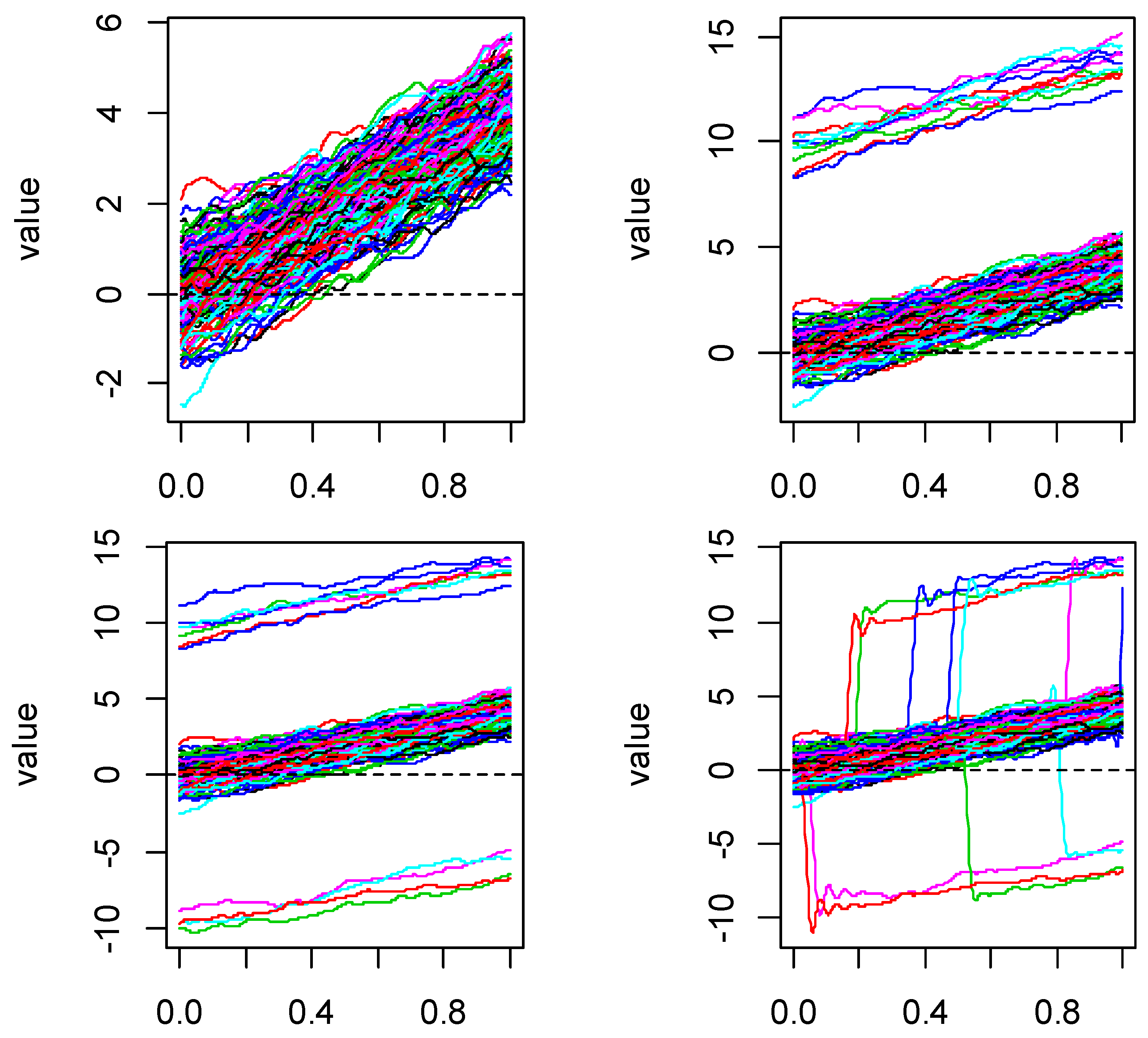
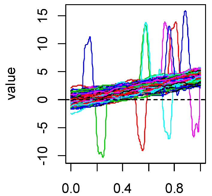
Figure 1 shows the simulated curves of these five models. For each model, we set 100 equal-interval sampling points in [0,1] and generated 200 replications. For Model 1, the parameter q was 0 and the contamination constant M was 0. For several other contaminated models, we considered several levels of contamination, with q = 5% and 10% and contamination constants M = 5 and 10. When fitting function curves, we use generalized cross validation (GCV) to obtain the number of bases. The results showed that the number of bases of Model 1–3 were the same, while those of Models 4 and 5 were different. However, due to the need of calculating the change of principal component coefficient, we had to calculate it on the same basis. Therefore, for comparison purposes, in Models 4 and 5, we selected the same number of bases as that of Model 1.
Classical L2-norm FPCA and L1-norm FPCA were used for the simulated functional data corresponding to these five models. We focused on their robust to various abnormal disturbances. When implementing L1-norm FPCA on Model 1, by comparing the value of objective function, the initial value was chosen as the first L2-norm functional principal component weight function, i.e., β 0 ( t ) = ξ ( t ) , where ξ ( t ) is the eigenfunction corresponding to the largest eigenvalue of the sample covariance function of the functional data in Model 1. Because the L1-norm FPCA of the following several disturbance models should be compared with Model 1, in order to ensure the consistency of conditions when calculating the L1-norm FPCA of the following several disturbance models, the initialization values also adopted the eigenfunction corresponding to the largest eigenvalue of the sample covariance function of the corresponding functional data.
The sums of absolute values of the coefficient differences of several principal components under non-contamination and contamination were compared and analyzed. The sum of the absolute values of the corresponding coefficient changes are given in Table 1, Table 2, Table 3 and Table 4. Since the variance contribution rate of the first principal component reached 80%, only the first principal component function was taken in Models 1, 2, 3 and 4. However, in order to achieve a similar variance contribution rate, at least four principal components were needed in Model 5. Thus, for Models 1, 2, 3 and 4, we only show the changes of the first principal component function. For Model 5, we show the changes of the first four principal component functions.
It can be seen from Table 1, Table 2, Table 3 and 
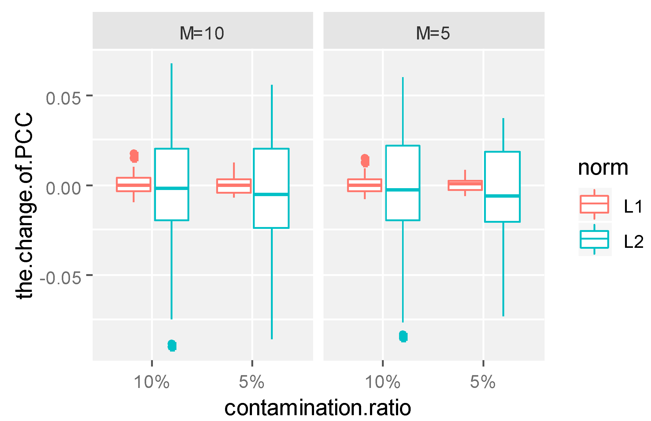
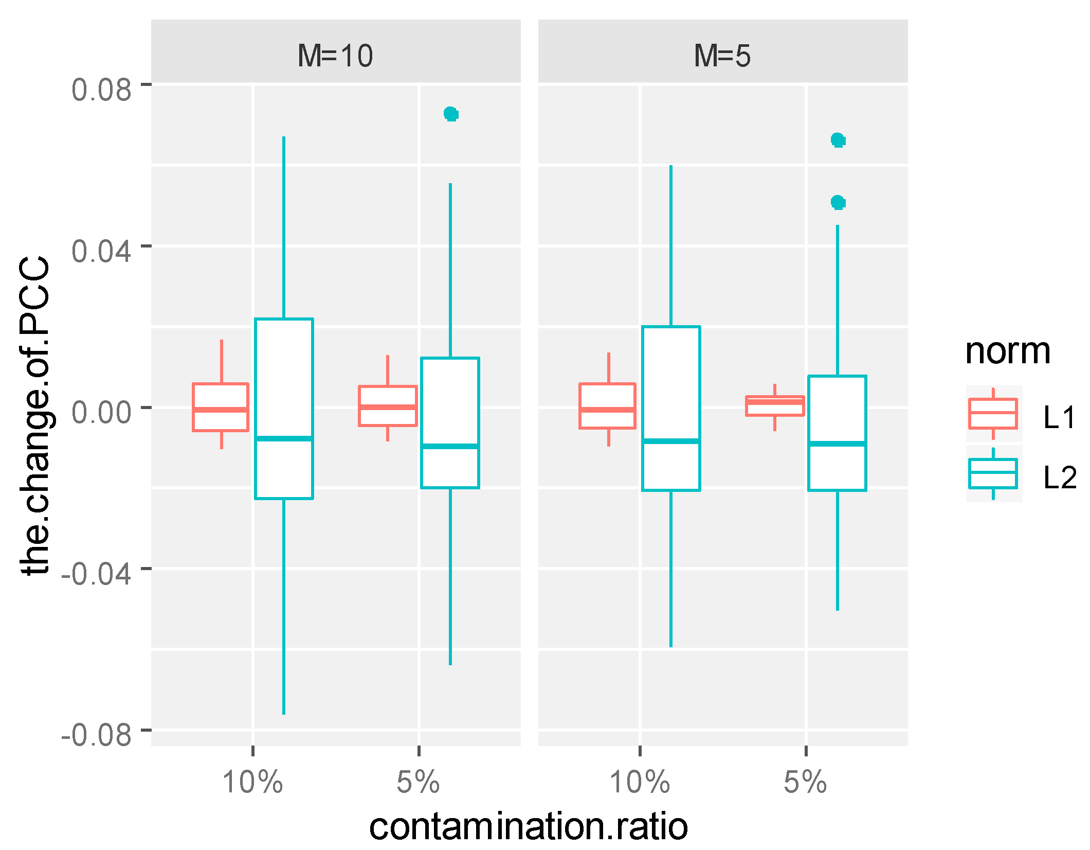
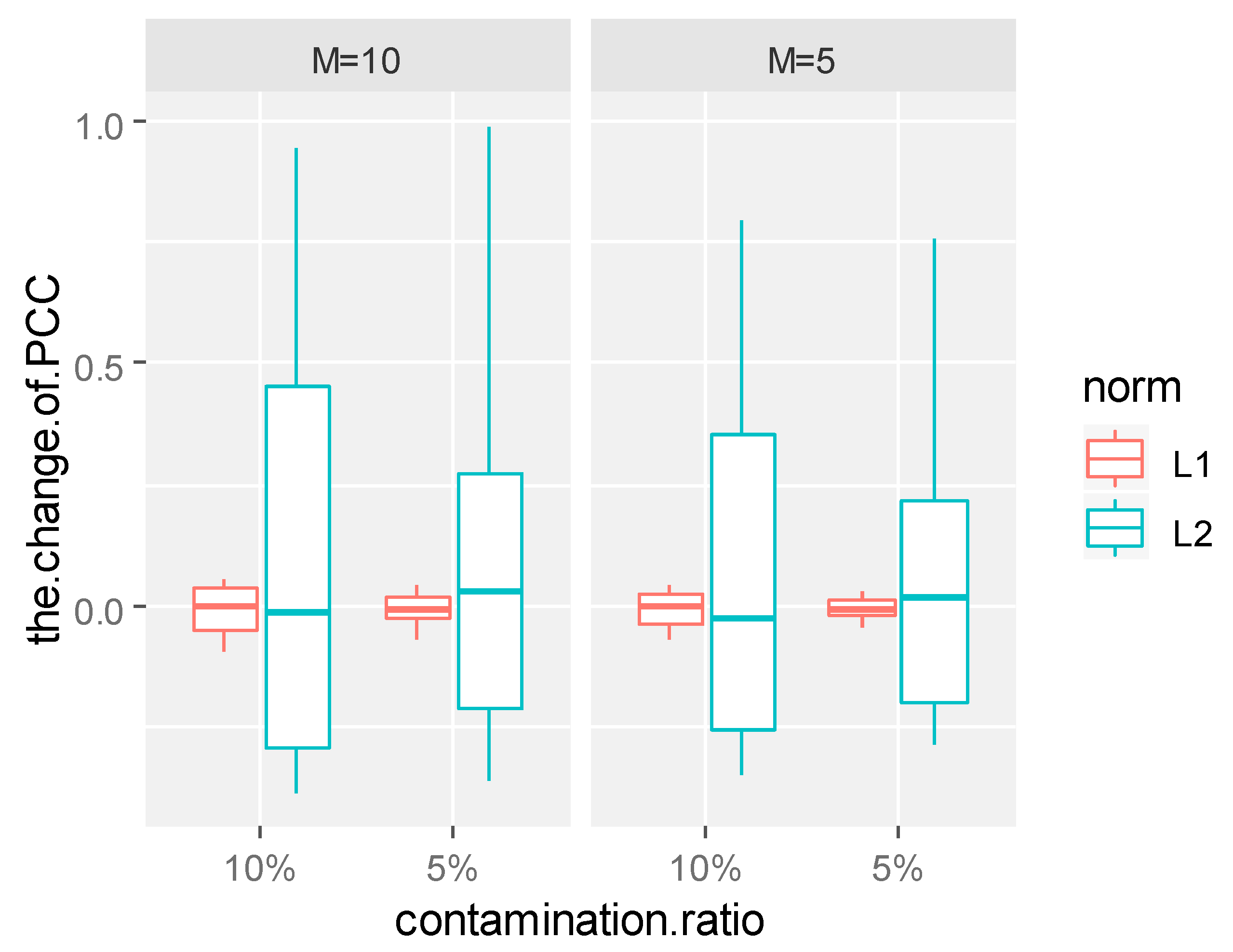
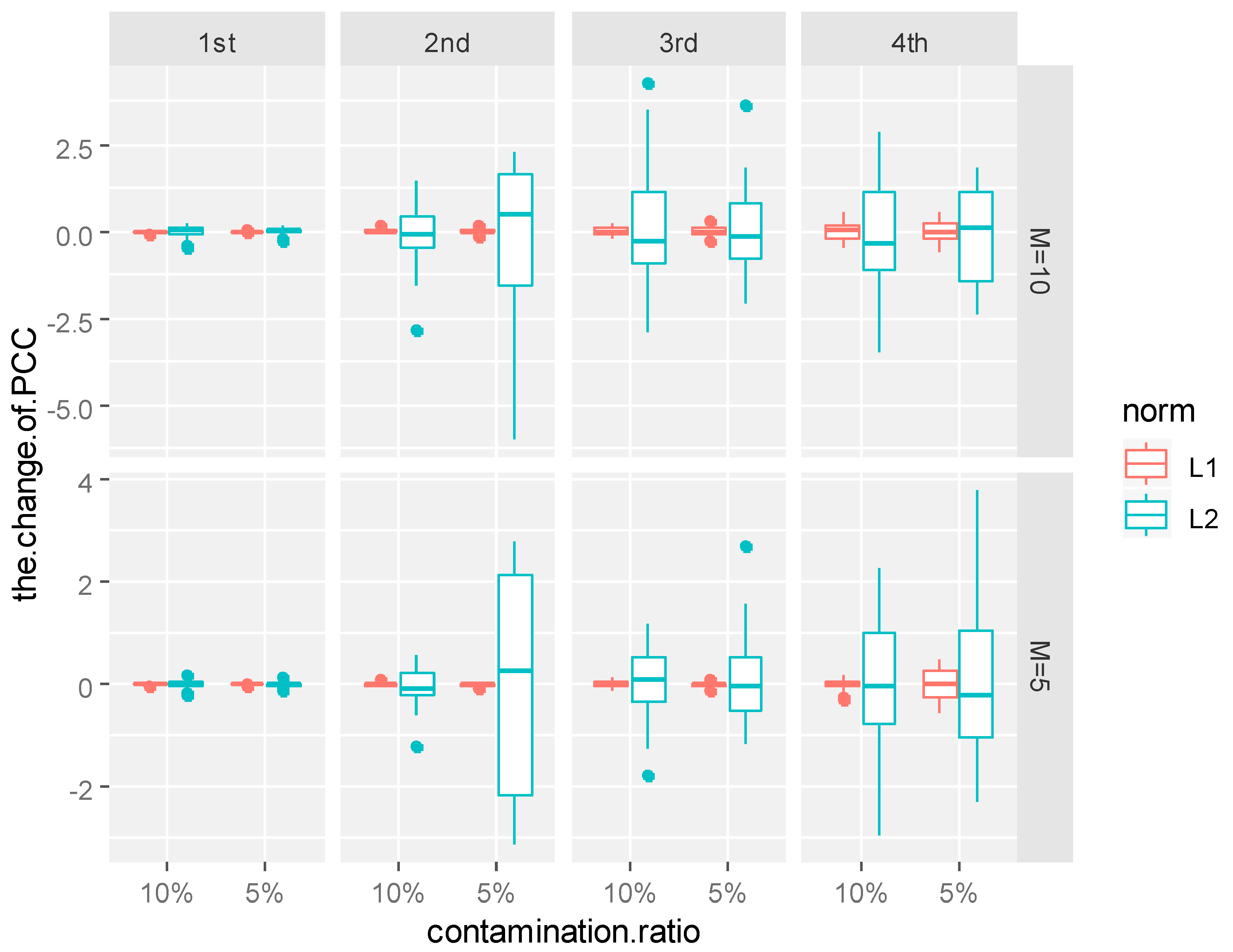
Table 4 that under the same contamination ratio and contamination size, the coefficient changes of the principal component weight functions of the L1-norm were significantly smaller than those of the L2-norm, which shows that the functional principal components of the L1-norm were more stable than those of the L2-norm, no matter which form of contamination was received. This conclusion can also be confirmed from the boxplots of the coefficient changes of the principal component weight functions.
As can be seen from Figure 2, Figure 3, Figure 4 and Figure 5, in the same contamination ratio and size, the changes of L1-norm principal component coefficient are more concentrated near zero compared with the changes of the L2-norm principal component coefficient, which shows that under the same contamination mode, L1-norm functional principal components were more robust to outliers and more reliable.
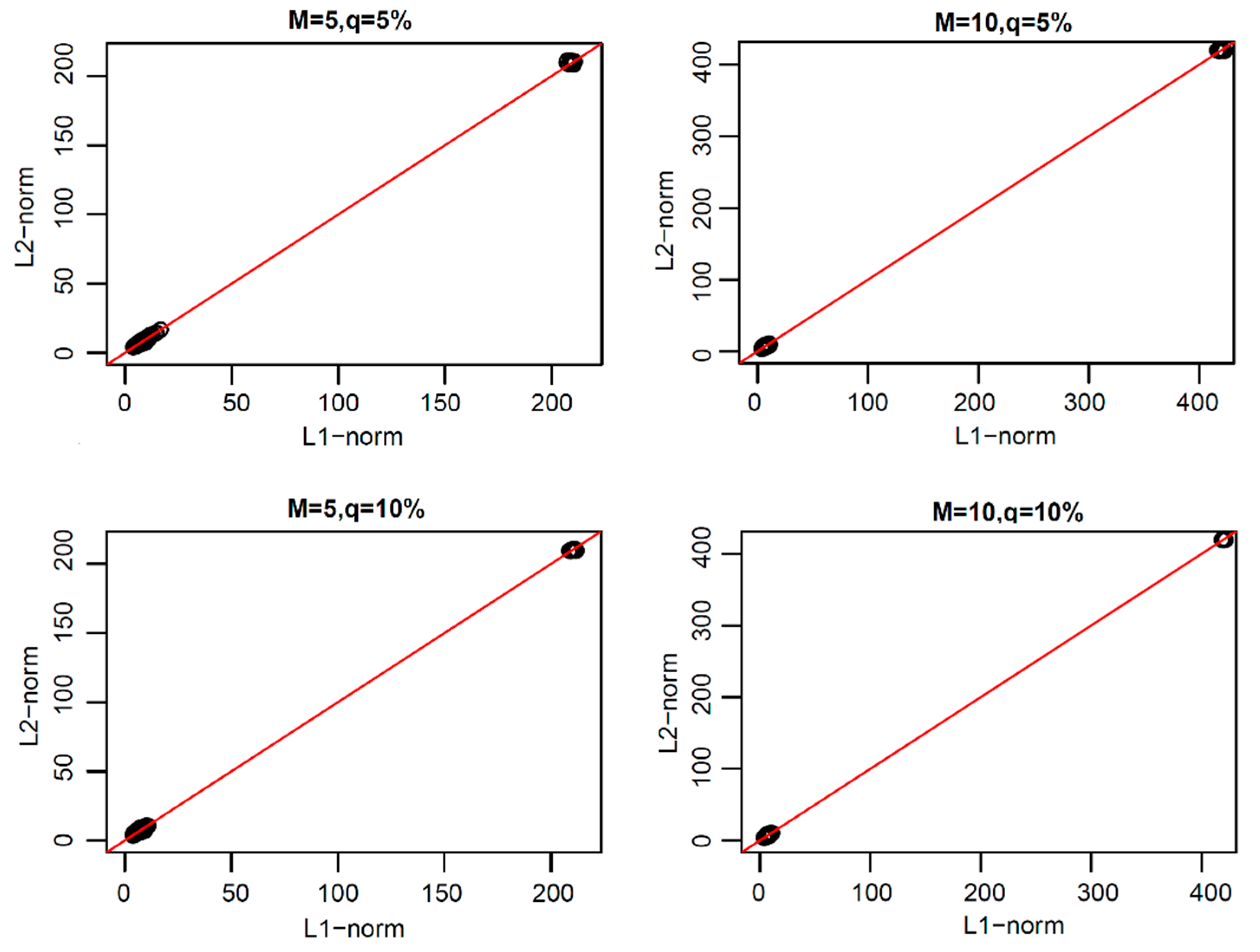
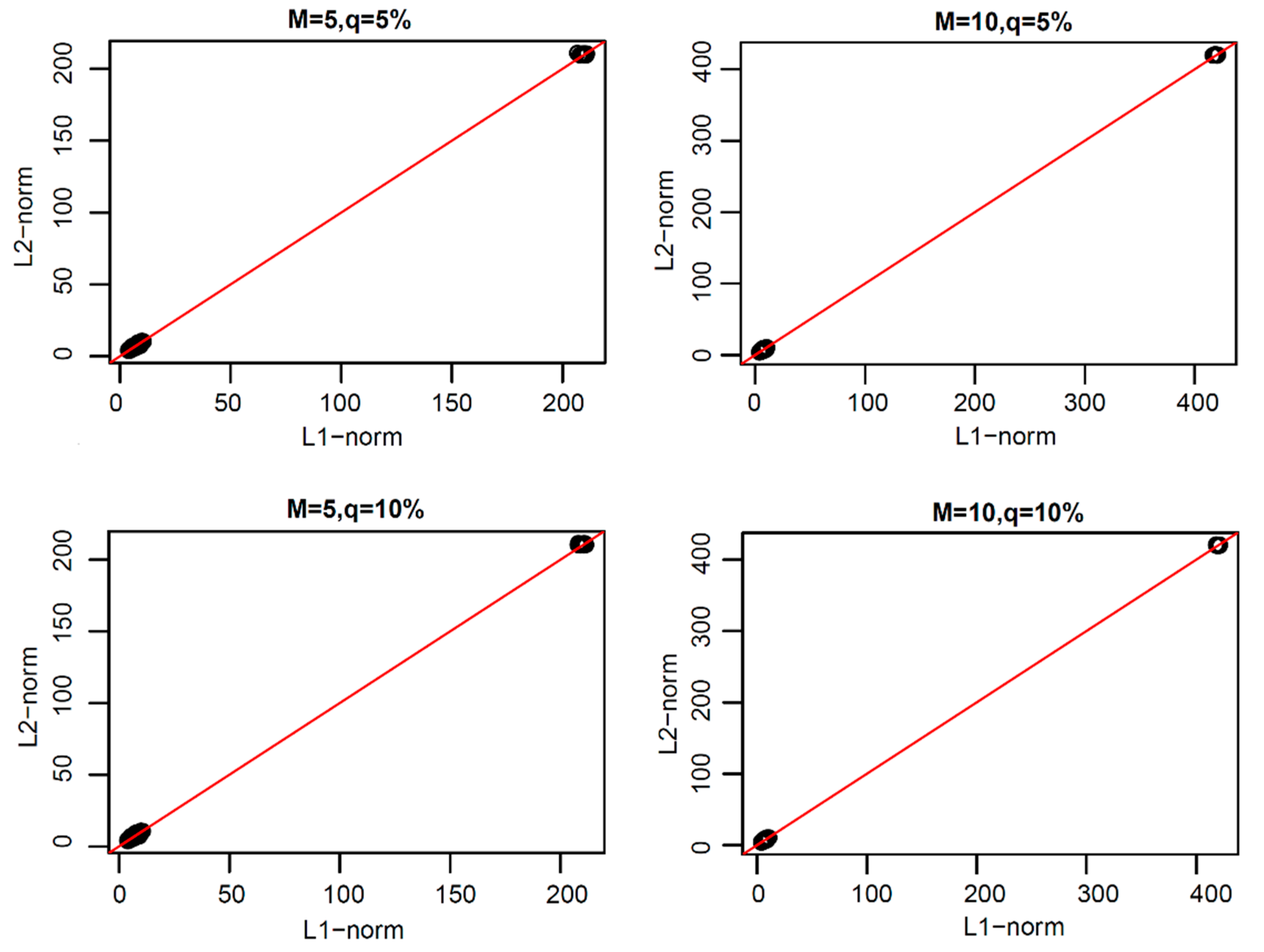
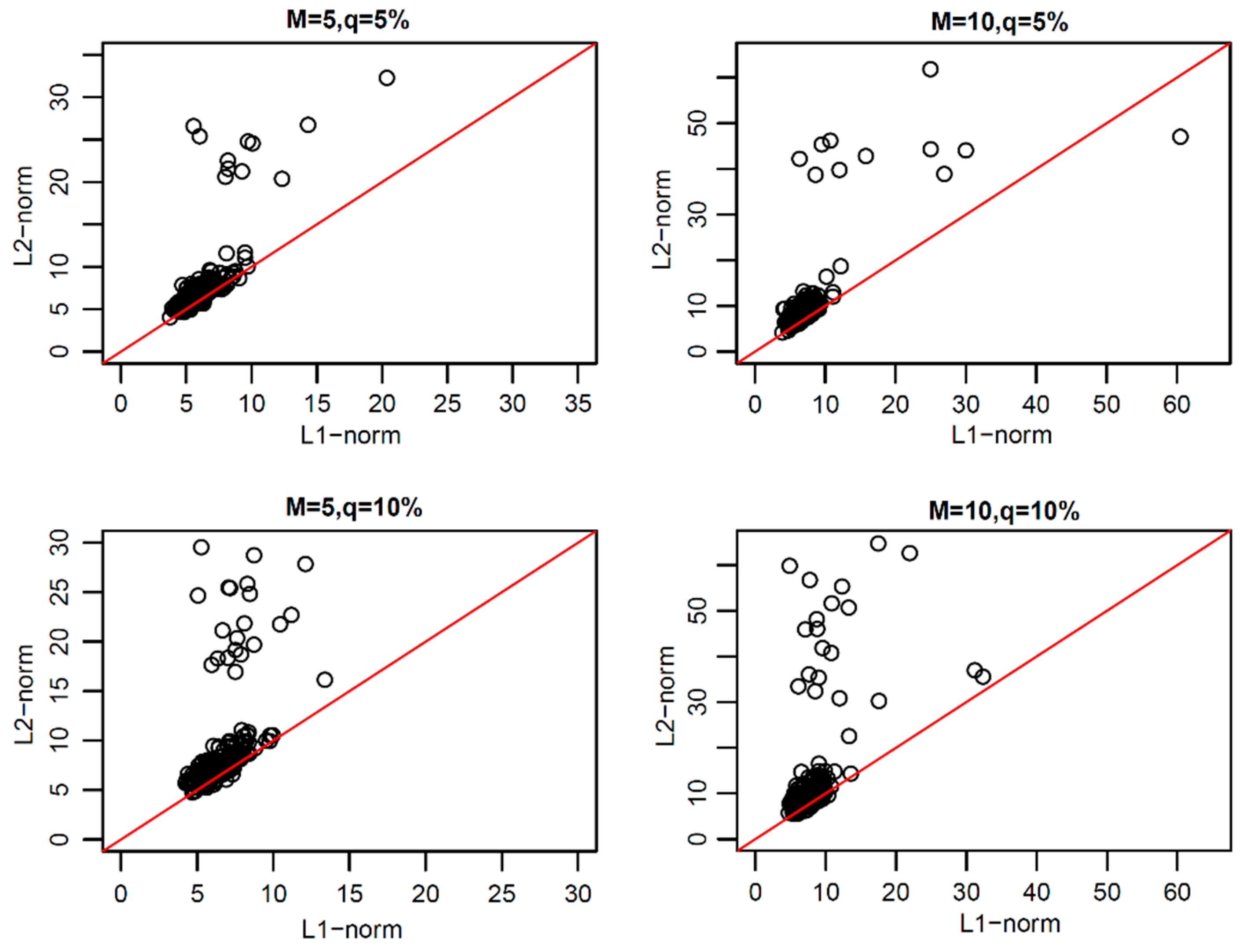
From the above research, we found that the L1-norm functional principal components were more robust than L2-norm functional principal components. Thus, how can one reconstruct the original functional data with these two types of principal components? In order to study this problem, we reconstructed the original uncontaminated functional data with the same number of functional principal components of L1-norm and L2-norm under each model. The scatter plots of the coefficients of the two types of reconstructed error curves are shown in Figure 6, Figure 7, Figure 8 and Figure 9.
In Figure 6, Figure 7, Figure 8 and Figure 9, we can see that the scatter plots of the reconstruction error curve coefficients of L1-norm and L2-norm were always near the line y = x under the first three pollution models, and under peak pollution, the reconstruction error of the L1-norm was smaller than that of the L2-norm. When using the paired one-sided T-test, the p-values were found to all be close to 1, indicating that the reconstruction error curve coefficients of the L1-norm were not greater than those of the L2-norm. Thus, the reconstruction ability of the L1-norm principal components to the original uncontaminated functional data was not worse than that of the L2-norm principal components. The results of the paired one-sided T-test are shown in Table 5, Table 6, Table 7 and Table 8.
The above experiments showed that the functional principal component of the L1-norm was not just stable and reliable, it also had the same reconstruction ability as the L2-norm.

4.2. Canadian Weather Data

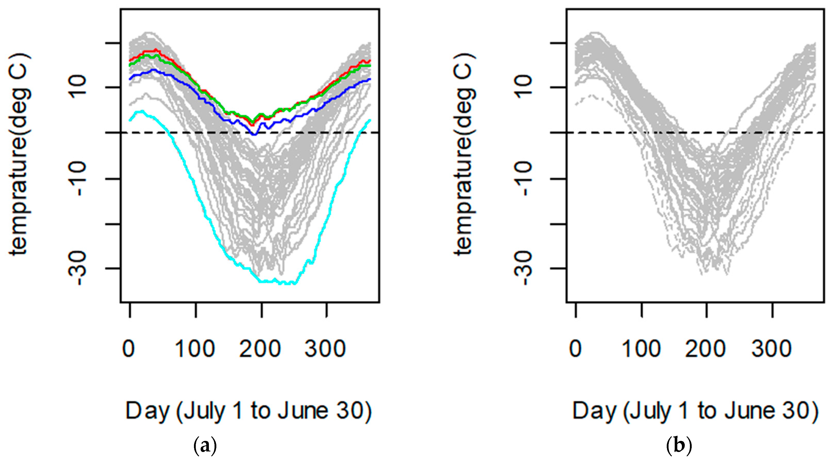
We used Canadian weather data, which provide daily temperatures at 35 different locations in Canada averaged over 1960–1994, in order to compare the robust to outliers of the L1-norm functional principal components and L2-norm functional principal components when the functional data were contaminated by abnormal data. Firstly, by considering the periodic characteristics of the data, the discrete temperature observation data were fitted into 35 functional curves by a Fourier basis function, and the number of the basis functions was 65. The fitting curves are shown in Figure 10a. As can be seen when using the function data outlier detection method [39], the temperature modes of the four stations of Vancouver, Victoria, Pr. Rupert and Resolute were different from those of the other stations. Figure 10b shows this function after removing the data from these four observatories. The functional data of the 35 observatories were called the whole data, and the functional data after removing Vancouver, Victoria, Pr. Rupert and Resolute were normal data, so the whole data can be understood as the addition of abnormalities to the normal data.
In order to compare the robustness between the L2-norm functional principal component weighting functions and the L1-norm functional principal component weighting functions to outliers, the L2-norm functional principal components and L1-norm functional principal components were, respectively, used for normal data and data added with outliers. For each method, the results of the two cases were compared, because the variance contribution rate of the first two principal components reached 90%, though the latter analysis only focused on the first two functional principal components.
Figure 11 shows the change of the first principal component weight function before and after adding outliers by using two functional principal component analysis methods. Figure 11a is a graph of the first principal component weight function that was obtained by using the L2-norm functional principal component method. The solid line is the result of normal data, and the dashed line is the result of adding four abnormal curves. Figure 11b is a graph of the first principal component weight function that was obtained by using the proposed L1-norm functional principal component method. After comparing the objective function, the initial value was chosen as the first L2-norm functional principal component weight function, i.e., β 0 ( t ) = ξ ( t ) , where ξ ( t ) is the eigenfunction corresponding to the largest eigenvalue of the sample covariance function of normal functional data and the same method for whole functional data. The solid line is the result of normal data, and the dashed line is the result of adding four abnormal curves. By comparing the coefficients of the two first functional principal component weighting functions, it was found that the sum of the absolute change of the coefficients of the first principal component weighting functions that were obtained by the L1-norm method before and after adding abnormal values was 0.16, which was less than the 0.18 corresponding to the L2-norm. Next, the performance of the second principal component weight function is discussed.
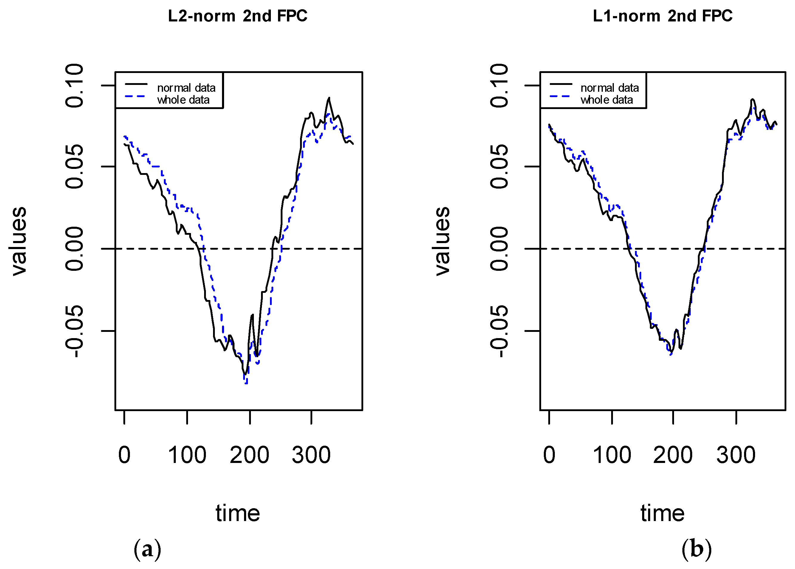
Figure 12 shows the change of the second principal component weight function before and after the addition of outliers by using two functional principal component analysis methods. Figure 12a is a graph of the second principal component weight function that was obtained by using the L2-norm function principal component method. The solid line is the result of normal data, and the dashed line is the result of adding four abnormal curves. Figure 12b is a graph of the second principal component weight function that was obtained by using the proposed L1-norm function principal component method. The solid line is the result of normal data, and the dashed line is the result of adding four abnormal curves. By comparing the coefficients of the two second function principal component weighting functions, it was found that the sum of absolute change of the coefficients of the second principal component weighting functions that were obtained by the L1-norm method before and after adding abnormal values was 0.33, which was less than the 0.76 corresponding to the L2-norm. the sums of the absolute values of the coefficient change of the principal component weight functions under the two methods are shown in Table 5.
Table 9 shows that the classical L2-norm principal components weight functions greatly changed before and after removing outliers, reflecting its sensitivity to outliers. However, the L1-norm functional principal components weight functions presented in this paper had little change before and after adding abnormal values. Therefore, that the L1-norm principal component weight function proposed in this paper has a strong anti-noise ability and a good stability.
We also compared the reconstruction ability of two types of principal components to normal data. The scatter plots of the coefficients of the two types of reconstructed error curves are shown in Figure 13.
From Figure 13, it can be seen the scatter plots of the reconstruction error curve coefficients of L1-norm and L2-norm were always near the line y = x; When we performed a paired one-sided T-test for the two groups of reconstruction error curve coefficients, the t value was found to 1.0323, the degree of freedom for the t-statistic was 33, and the p-value was 0.1547, which indicates that the reconstruction error curve coefficients of L1-norm were not greater than those of L2-norm. Thus, the reconstruction ability of the L1-norm principal components to the original uncontaminated functional data was not worse than the L2-norm principal components.

5. Concluding Remarks

FPCA is a primary step for functional data exploration, and the reliability of FPCA plays an important role in subsequent analysis. The existing principal component methods of functional data were established in an L2-norm framework. However, because the L2-norm enlarges the influence of outliers, the traditional functional principal components analysis method is sensitive to outliers. On the other hand, in regard to multivariate data, the relevant research on the principal component analysis method [30,31,32,33,34,35,36,37] have shown that the principal component analysis method of L1-norm for multivariate data has a better robustness than that of the L2-norm. Motivated by this research, in this paper, we tried to construct an L1-norm principal component analysis method for functional data. Firstly, we built a functional data L1-norm maximized principal component optimization model. Then, a corresponding algorithm for solving the L1-norm maximized optimization model was constructed based on the idea of multivariate data L1-norm principal component analysis method [30]. An extensive simulation study was conducted, and a real dataset of Canadian weather was employed to assess the robustness of the L1-norm functional principal component analysis. From the simulation study that considered different contamination configurations (symmetric, asymmetric, partial and peak), we found that the L1-norm functional principal component analysis method provides a more robust estimation of principal components than the traditional L2-norm principal component analysis method. Finally, by comparing the reconstruction errors of the L1-norm FPCA and L2-norm FPCA, it was found that the reconstruction ability of the L1-norm principal components to the original uncontaminated functional data is as good as that of the L2-norm principal components. Therefore, when functional data contain outliers, the estimation given by the L1-norm functional principal component analysis method is more reliable. The proposed L1-norm FPCA may prove to be an useful addition to functional data analysis.

Author Contributions

Individual contributions to this article: conceptualization, F.Y. and L.L.; methodology, F.Y. and L.L.; software, L.J. and D.Q.; validation, F.Y. and N.Y.; writing—original draft preparation, F.Y. and L.L.; writing—review and editing, F.Y. and L.L.; supervision, L.L. All authors have read and agreed to the published version of the manuscript.

Funding

This work was supported in part by the Beijing Natural Science Foundation under Grant No.9172003, in part by the National Natural Science Foundation of China under Grant No. 61876200, in part by the Natural Science Foundation Project of Chongqing Science and Technology Commission under Grant No. cstc2018jcyjAX0112.

Acknowledgments

The authors thank the anonymous referees for their careful reading and helpful suggestions, which help to improve the quality of this paper.

Conflicts of Interest

The authors declare no conflicts of interest.

References

  1. Kowal, D.R. Integer-valued functional data analysis for measles forecasting. Biometric 2019, in press. [Google Scholar] [CrossRef] [PubMed]
  2. Wagner-Muns, I.M.; Guardiola, I.G.; Sama-ranayke, V.A.; Kayani, W.I. A functional data analysis approach to traffic volume forecasting. IEEE Trans. Intell. Transp. Syst. 2017, 19, 878–888. [Google Scholar] [CrossRef]
  3. Ramsay, J.O.; Silverman, B.W. Applied functional data analysis. J. Educ. Behav. Stat. 2008, 24, 5822–5828. [Google Scholar]
  4. Yao, F.; Müller, H.G.; Wang, J.L. Functional data analysis for sparse longitudinal data. J. Am. Stat. Assoc. 2005, 100, 577–590. [Google Scholar] [CrossRef]
  5. Auton, T. Applied functional data analysis: Methods and case studies. J. R. Stat. Soc. 2010, 167, 378–379. [Google Scholar] [CrossRef]
  6. Zambom, A.Z.; Collazos, J.A.; Dias, R. Functional data clustering via hypothesis testing k-means. Comput. Stat. 2019, 34, 527–549. [Google Scholar] [CrossRef]
  7. Ferraty, F.; Vieu, P. Nonparametric Functional Data Analysis: Theory and Practice; Springer Science & Business Media: Berlin, Germany, 2006. [Google Scholar]
  8. Horváth, L.; Kokoszka, P. Inference for Functional Data with Applications; Springer Science & Business Media: Berlin, Germany, 2012; Volume 200. [Google Scholar]
  9. Tarpey, T.; Kinateder, K.K. Clustering functional data. J. Classif. 2003, 20, 93–114. [Google Scholar] [CrossRef]
  10. Ramsay, J.O.; Silverman, B.W. Applied Functional Data Analysis: Methods and Case Studies; Springer: Berlin/Heidelberg, Germany, 2007. [Google Scholar]
  11. Estévez-Pérez, G.; Vilar, J.A. Functional anova starting from discrete data: An application to air quality data. Environ. Ecol. Stat. 2013, 20, 495–517. [Google Scholar] [CrossRef]
  12. Ignaccolo, R.; Ghigo, S.; Giovenali, E. Analysis of air quality monitoring networks by functional clustering. Environmetrics 2010, 19, 672–686. [Google Scholar] [CrossRef]
  13. Ferraty, F.; Vieu, P. Nonparametric models for functional data, with application in regression, time series prediction and curve discrimination. Nonparametr. Stat. 2004, 16, 111–125. [Google Scholar] [CrossRef]
  14. Febrero, M.; Galeano, P.; González-Manteiga, W. Outlier detection in functional data by depth measures, with application to identify abnormal nox levels. Environmetrics 2010, 19, 331–345. [Google Scholar] [CrossRef]
  15. Ratcliffe, S.J.; Heller, G.Z.; Leader, L.R. Functional data analysis with application to periodically stimulated foetal heart rate data ii functional logistic regression. Stat. Med. 2002, 21, 1103–1114. [Google Scholar] [CrossRef] [PubMed]
  16. Giraldo, R.; Delicado, P.; Mateu, J. Continuous time-varying kriging for spatial prediction of functional data: An environmental application. J. Agric. Biol. Environ. Stat. 2010, 15, 66–82. [Google Scholar] [CrossRef]
  17. Ferraty, F.; Rabhi, A.; Vieu, P. Conditional quantiles for dependent functional data with application to the climatic “el niño” phenomenon. Sankhyā Indian J. Stat. 2005, 67, 378–398. [Google Scholar]
  18. Baladandayuthapani, V.; Mallick, B.K.; Young Hong, M.; Lupton, J.R.; Turner, N.D.; Carroll, R.J. Bayesian hierarchical spatially correlated functional data analysis with application to colon carcinogenesis. Biometrics 2008, 64, 64–73. [Google Scholar] [CrossRef] [Green Version]
  19. Ramsay, J.O.; Dalzell, C.J. Some tools for functional data analysis. J. R. Stat. Soc. 1991, 53, 539–572. [Google Scholar] [CrossRef]
  20. Ramsay, J.O. Functional data analysis. Encycl. Stat. Sci. 2004, 4. [Google Scholar] [CrossRef]
  21. Dauxois, J.; Pousse, A.; Romain, Y. Asymptotic theory for the principal component analysis of a vector random function: Some applications to statistical inference. J. Multivar. Anal. 1982, 12, 136–154. [Google Scholar] [CrossRef] [Green Version]
  22. Rice, J.A.; Silverman, B.W. Estimating the mean and covariance structure nonparametrically when the data are curves. J. R. Stat. Soc. 1991, 53, 233–243. [Google Scholar] [CrossRef]
  23. Levy, A.; Rubinstein, J. Some properties of smoothed principal component analysis for functional data. J. Opt. Soc. Am. 1999, 16, 28–35. [Google Scholar] [CrossRef]
  24. Silverman, B.W. Smoothed functional principal components analysis by choice of norm. Ann. Stat. 1996, 24, 1–24. [Google Scholar] [CrossRef]
  25. James, G.M.; Hastie, T.J.; Sugar, C.A. Principal component models for sparse functional data. Biometrika 2000, 87, 587–602. [Google Scholar] [CrossRef] [Green Version]
  26. Boente, G.; Fraiman, R. Kernel-based functional principal components. Stat. Probab. Lett. 2000, 48, 335–345. [Google Scholar] [CrossRef]
  27. Hall, P.; Hosseini-Nasab, M. On properties of functional principal components analysis. J. R. Stat. Soc. Ser. B Stat. Methodol. 2006, 68, 109–126. [Google Scholar] [CrossRef]
  28. Benko, M.; Härdle, W.; Kneip, A. Common functional principal components. Ann. Stat. 2009, 37, 1–34. [Google Scholar] [CrossRef]
  29. Hörmann, S.; Kidziński, Ł.; Hallin, M. Dynamic functional principal components. J. R. Stat. Soc. Ser. B Stat. Methodol. 2015, 77, 319–348. [Google Scholar] [CrossRef]
  30. Kwak, N. Principal component analysis based on l1-norm maximization. IEEE Trans. Pattern Anal. Mach. Intell. 2008, 30, 1672–1680. [Google Scholar] [CrossRef]
  31. Nie, F.; Huang, H.; Ding, C.; Luo, D.; Wang, H. Robust principal component analysis with non-greedy ℓ1-norm maximization. In Proceedings of the Twenty-Second International Joint Conference on Artificial Intelligence, Barcelona, Spain, 16–22 July 2011. [Google Scholar]
  32. Markopoulos, P.P.; Karystinos, G.N.; Pados, D.A. Optimal algorithms for L1-subspace signal processing. IEEE Trans. Signal Process. 2014, 62, 5046–5058. [Google Scholar] [CrossRef]
  33. Markopoulos, P.P.; Kundu, S.; Chamadia, S.; Pados, D.A. Efficient L1-norm principal-component analysis via bit flipping. IEEE Trans. Signal Process. 2017, 65, 4252–4264. [Google Scholar] [CrossRef]
  34. Martin-Clemente, R.; Zarzoso, V. On the link between L1-PCA and ICA. IEEE Trans. Pattern Anal. Mach. Intell. 2016, 39, 515–528. [Google Scholar] [CrossRef]
  35. Park, Y.W.; Klabjan, D. Iteratively reweighted least squares algorithms for L1-norm principal component analysis. In Proceedings of the 2016 IEEE 16th International Conference on Data Mining (ICDM), Barcelona, Spain, 12–15 December; IEEE: Piscataway, NJ, USA, 2016. [Google Scholar]
  36. Markopoulos, P.P.; Dhanaraj, M.; Savakis, A. Adaptive L1-norm principal-component analysis with online outlier rejection. IEEE J. Sel. Top. Signal Process. 2018, 12, 1131–1143. [Google Scholar] [CrossRef]
  37. Tsagkarakis, N.; Markopoulos, P.P.; Pados, D.A. On the L1-norm approximation of a matrix by another of lower rank. In Proceedings of the 2016 15th IEEE International Conference on Machine Learning and Applications (ICMLA), Anaheim, CA, USA, 18–20 December 2016; IEEE: Piscataway, NJ, USA, 2016. [Google Scholar]
  38. Fraiman, R.; Muniz, G. Trimmed means for functional data. Test 2001, 10, 419–440. [Google Scholar] [CrossRef]
  39. Yu, F.; Liu, L.; Jin, L.; Yu, N.; Shang, H. A method for detecting outliers in functional data. In Proceedings of the IECON 2017-43rd Annual Conference of the IEEE Industrial Electronics Society, Beijing, China, 29 October–1 November 2017; IEEE: Piscataway, NJ, USA, 2017; pp. 7405–7410. [Google Scholar]
Figure 1. Curves generated from Model 1 (without contamination), Model 2 (asymmetric contamination), Model 3 (symmetric contamination), Model 4 (partial contamination) and Model 5 (peak contamination) with n = 200, p = 100, q = 5% and M = 10.
Symmetry 12 00182 g001aSymmetry 12 00182 g001b
Figure 2. The boxplots of the change of the first principal component coefficient for asymmetric contamination (q = 5% and q = 10%; M = 5 and M = 10).
Symmetry 12 00182 g002
Figure 3. The boxplots of the change of the first principal component coefficient for symmetric contamination (q = 5% and q = 10%; M = 5 and M = 10).
Symmetry 12 00182 g003
Figure 4. The boxplots of the change of the first principal component coefficient for partial contamination (q = 5% and q = 10%; M = 5 and M = 10).
Symmetry 12 00182 g004
Figure 5. The boxplots of the change of the first four principal component coefficient for peak contamination (q = 5% and q = 10%; M = 5 and M = 10).
Symmetry 12 00182 g005
Figure 6. Scatter plots of the coefficients of the reconstruction error curves of L1-norm and L2-norm under asymmetric contamination.
Symmetry 12 00182 g006
Figure 7. Scatter plots of the coefficients of the reconstruction error curves of L1-norm and L2-norm under symmetric contamination.
Symmetry 12 00182 g007
Figure 8. Scatter plots of the coefficients of the reconstruction error curves of L1-norm and L2-norm under partial contamination.
Symmetry 12 00182 g008
Figure 9. Scatter plots of the coefficients of the reconstruction error curves of L1-norm and L2-norm under peak contamination.
Symmetry 12 00182 g009
Figure 10. Daily mean temperature curves of 35 observatories in Canada ((a) whole data, (b) normal data).
Symmetry 12 00182 g010
Figure 11. The first principal component weight function for normal data and whole data. (a) L2-norm, (b) L1-norm.
Symmetry 12 00182 g011
Figure 12. The second principal component weight function for normal data and whole data. (a) L2-norm, (b) L1-norm
Symmetry 12 00182 g012
Figure 13. Scatter plot of reconstruction error curve of L1-norm and L2-norm to normal data.
Symmetry 12 00182 g013
Table 1. The sum of the absolute values of the first principal component weight function coefficient changes for no contamination and asymmetric contamination (5% and 10%).
M = 10M = 5
qL1-norm FPCL2-norm FPCL1-norm FPCL2-norm FPC
1st FPC1st FPC1st FPC1st FPC
5%0.171.130.130.91
10%0.221.240.181.16
Table 2. The sum of the absolute values of the first principal component weight function coefficient changes for no contamination and symmetric contamination (5% and 10%).
M = 10 M = 5
qL1-norm FPCL2-norm FPCL1-norm FPCL2-norm FPC
1st FPC 1st FPC 1st FPC 1st FPC
5%0.2 1.13 0.1 0.96
10%0.251.170.231.04
Table 3. The sum of the absolute values of the first principal component weight function coefficient changes for no contamination and partial contamination (5% and 10%).
M = 10 M = 5
qL1-norm FPCL2-norm FPCL1-norm FPCL2-norm FPC
1st FPC 1st FPC 1st FPC 1st FPC
5%1.17 13.47 0.81 10.67
10%1.7014.771.2412.29
Table 4. The sum of the absolute values of the first four principal component weight functions. Coefficient changes for no contamination and peak contamination (5% and 10%).
M = 10M = 5
qL1-norm FPCL2-norm FPCL1-norm FPCL2-norm FPC
1st2nd3rd4th1st2nd3rd4th1st2nd 3rd4th1st2nd3rd4th
5%0.51.53.99.83.966.339.245.20.20.71.310.13.966.839.945.7
10%0.81.84.18.45.424.248.454.30.41.22.23.42.310.922.342.2
Table 5. The table of the one-sided paired T-test of the coefficients of the reconstruction error curves of L1-norm and L2-norm under asymmetric contamination (Alternative hypothesis: The true difference of the reconstruction error curve coefficients of L1-norm and L2-norm in means was greater than 0.).
qM = 5M = 10
tdfp-Valuetdfp-Value
5%−2.84471990.9975−2.16511990.9842
10%−2.24841990.9872−2.58431990.9948
Table 6. The table of the one-sided paired T-test of the coefficients of the reconstruction error curves of L1-norm and L2-norm under symmetric contamination (Alternative hypothesis: The true difference of the reconstruction error curve coefficients of L1-norm and L2-norm in means was greater than 0.).
qM = 5M = 10
tdfp-Valuetdfp-Value
5%−3.87611990.9999−3.341990.9995
10%−4.76281991−3.52931990.9997
Table 7. The table of the one-sided paired T-test of the coefficients of the reconstruction error curve of L1-norm and L2-norm under partial contamination (Alternative hypothesis: The true difference of the reconstruction error curve coefficients of L1-norm and L2-norm in means was greater than 0.).
qM = 5M = 10
tdfp-Valuetdfp-Value
5%−5.23731991−4.93711991
10%−7.78961991−5.0331991
Table 8. The table of the one-sided paired T-test of the coefficients of the reconstruction error curves of L1-norm and L2-norm under peak contamination (Alternative hypothesis: The true difference of the reconstruction error curve coefficients of L1-norm and L2-norm in means was greater than 0.).
qM = 5M = 10
tdfp-Valuetdfp-Value
5%−6.65021991−6.62121991
10%−7.63131991−6.85641991
Table 9. The sum of absolute change of the coefficients of the first two principal component weighting functions.
The Sum of Absolute Change of the CoefficientsThe 1st Function Principal Component Weighting FunctionThe 2nd Function Principal Component Weighting Function
L2-norm0.180.76
L1-norm 0.160.33

