1. Introduction
The success and sustainability of each economic system is directly dependent on the ability to finance all capital projects considering different areas. In such a system, the banking sector can play a key role, especially when it comes to developing countries. The banking sector is the most important part of both the financial and economic systems of every country. Banks play a key role in financial intermediation through the following processes: asset mobilization, asset allocation, investment of national savings and other forms of capital. The extent to which the banking sector is developed within the country’s financial system influences how efficient the allocation of capital will be, how dynamic the growth of the enterprise will be, and how expansive the overall economic development will be. It is evident that the banking sector in many countries has been experiencing financial difficulties of varying intensity in recent decades. These phenomena have particularly appeared in the past two decades, so the serious financial troubles have plagued many countries.
One of the ways to overcome the problems of financial crises and maintain confidence in the banking sector of countries is to determine the real quality of individual banks that are participants in the market. A clear picture of participants allows both the corporate and the retail sectors to avoid the pitfalls of malicious marketing and problematic business behavior. In addition, the reliance on high-quality participants in the banking sector and the elimination of those who are not, is the first prerequisite for the smooth functioning of the economy and its continued growth and development. Accordingly, there is a real requirement to form an adequate model that will best assess the quality of each unit and, as a result, provide a complete ranking list of all banks ranked. The problem of ranking alternatives, i.e., banks in the particular case, is based on a large number of “angles” from which it is necessary to consider the quality of a bank and then, on that basis, to construct a “global (integral) quality index” that enables cross-comparisons. The large amount of business data possessed by all companies, and thus by banks, further complicates this analysis and requires the selection of only the most significant indicators that realistically reflect the performance and quality of the business. In addition, the model would need to enable ranked participants to identify their weaknesses and, on that basis, to make certain adjustments to the business that would improve the lagged segments of the business.
In accordance with the above, and the methodology developed and applied in this paper, the following goals can be identified. The first goal is to enrich the area that addresses multi-criteria problems through the formation of an integrated subjective-objective model. The second goal of the paper is the possibility of constructing a multi-criteria model that should enable the ranking of banks as economic units, based on the most significant indicators of their business performance. The third goal of the paper involves a brief critique of the previous MCDM (multi-criteria decision-making) problems with an unbalanced hierarchical structure at lower levels of the hierarchy, which practically has a great influence on final decisions. The fourth goal of the paper is to enhance the integration of uncertainty theory, such as fuzzy logic, with other approaches, and the integration of subjective-objective models in order to achieve more accurate and approximately optimal results. As previously mentioned, we can synthesize one main goal of this research, in that such developed a model should ensure precise answer various questions and give potential approximately optimal solutions in various fields taking into account different constraints.
In addition to the introduction, conducted research is described through five more sections.
Section 2 focuses on the importance of a new approach to business excellence and a brief review of the situation in the field.
Section 3 presents a defined methodology of the paper and a research flow. This section integrates different approaches.
Section 4 summarizes the results, i.e., the ranking of banks on the basis of a previously extensive analysis and the multiphase determining the significance of the criteria used for the ranking. In
Section 5, the proposed model is verified, i.e., the results are obtained throughout a sensitivity analysis.
Section 6 includes concluding considerations with an overview of instructions for future research.
2. Literature Review
In recent decades, a new approach has been introduced to the business world, called “business excellence” (BE) in the literature. Facing an increasingly unstable and asymmetric business market, a large number of organizations are implementing BE strategies and quality systems as key elements of their business concept [
1] that lead to improved business results [
2]. The design, creation, implementation, and evaluation of these strategies require the reconsideration of how organizations work. The increasing application of different methods and tools, such as business process rearrangement, continuous monitoring of results, enterprise resource planning (ERP), lean management, or Six Sigma model management, have imposed the need for an integrated model in order to achieve BE at all levels in companies [
3].
BE can be seen not only as a new understanding of the quality system [
4], but also as an umbrella term that takes into account a broader range of issues like sustainability [
5].
Increasing competition in the banking sector [
6] has led banks to become actively involved in developing quality systems and business excellence in their business. This also appears as an inevitability since, according to Navid and Shabantaheri [
7], many people believe that the traditional method of banking is not flexible. By raising the quality level, banks seek to retain their customers and build a certain level of loyalty. In this way, through the improvement of quality, each bank develops its business [
8].
In order to determine the quality and the way of doing business, reports with indicators are formed for each bank separately according to different criteria. Following the adoption of reports, multi-criteria analysis methods are often applied to rank the banks and provide a clearer picture of comparative business. Stanujkic et al. [
9] ranked five commercial banks in Serbia using various methods, such as: simple additive weighting (SAW), additive ratio assessment (ARAS), COmplex PRoportional ASsessment (COPRAS), multi-objective optimization on the basis of ratio analysis (MOORA), gray relational analysis (GRA), compromise programming (CP), VIKOR (VIsekriterijumska optimizacija i KOmpromisno Resenje) and Technique for ordering preference by similarity to ideal solution (TOPSIS). In the research, they used the four most important criteria: liquidity, efficiency, profitability, and capital adequacy, consisting of three sub-criteria, and four sub-criteria for capital adequacy. They concluded that various aggregation and normalization procedures in some cases lead to obtaining the various optimal solutions. Considering this limitation and the impact on the final results, a more accurate subjective-objective model has been applied in this research.
Ratković et al. [
10] carried out a comparative quality analysis of the banking and postal sectors in Serbia by applying the SERVQUAL model based on five basic dimensions of customer expectations and perceptions. The findings of this study indicate that it is important to improve the situation regarding quality in the banking sector significantly. All dimensions of the SERVQUAL model need to be improved.
An integrated MCDM model consisting of four methods: Fuzzy AHP, TOPSIS, VIKOR and ELECTRE and Balance scorecard (BSC) was applied in [
11] to determine the performance of three banks in Iran on the basis of 21 evaluation indexes. In the study [
12], bank loan default classification models were evaluated using the TOPSIS method and the K-nearest neighbor algorithm. Wanke et al. [
13] evaluated the performance of the Association of Southeast Asian Nations banks based on the integration of the MCDM model involving fuzzy AHP, TOPSIS, and neural networks. In contrast to this research, they performed an evaluation based on CAMELS input parameters. CAMELS includes capital adequacy (C), asset quality (A), management quality (M), earnings (E), liquidity (L), and sensitivity to market risk (S). Gökalp [
14] applied the PROMETHEE (Preference Ranking Organization Method for Enrichment Evaluations) method to compare state, private and foreign banks located in the territory of Turkey. The authors analyzed the six-year period in order to obtain better and clearer results. He has obtained different results depending on the observation period, so it can be concluded that such an evaluation is necessary to perform periodically. The evaluation was based on the input parameters of the CAMEL system. The integration of AHP and TOPSIS methods is common, and the model has also been used in [
15] to evaluate private banks in Turkey. The research included 21 banks that were evaluated on the basis of financial parameters. Önder and Hepsen [
16] also applied the same combined AHP–TOPSIS model to evaluate Turkish banks over a nine-year period. A model of 57 criteria was created, based on which 17 banks were evaluated. The same model, but in fuzzy form [
17], was applied for the evaluation of 12 banks in the territory of Serbia, including 19 evaluation parameters. The combination of entropy and TOPSIS methods was used in [
18] to perform the evaluation of 12 banks based on five criteria: growth rate, number of branches, numbers of ATM, net income, and lending. Beheshtinia and Omidi [
19] applied (AHP) and modified digital logic (MDL) tools for determining the weight values of 23 criteria, while fuzzy TOPSIS and fuzzy VIKOR methods were implemented in the evaluation process of four banks in Iran. Since different approaches also provide differences in the rankings of alternatives, the Copeland method was used in the end to aggregate the results, i.e., the rankings of alternatives. Ginevičius and Podvezko [
20] state that one of the most significant criteria that has influence on the economic development of any organization is effective performance and bank reliability. Accordingly, they carried out a comparative analysis of ten commercial banks in Lithuania on the basis of 15 criteria. They applied various MCDM methods: SR (sum of ranks), SAW (simple additive weighting), TOPSIS and COPRAS (complex proportional assessment). In [
21], the integration of the AHP method with VIKOR was applied in order to evaluate banks in India.
Using different MCDM methods, in integration with other approaches such as fuzzy logic, is evidenced in the literature in a large number of examples [
22]. For example, such approach has been integrated with analytical network process (ANP), in order to improve quality in the airline industry [
23]. Dinçer and Yüksel in their study [
24] are evaluated BSC criteria with the integrated hybrid multicriteria decision-making approach by using fuzzy AHP, fuzzy ANP, and fuzzy VIseKriterijumska Optimizacija I Kompromisno Resenje (VIKOR) methods. Ecer [
25] in his paper combines the fuzzy AHP with the ARAS for development a new integrated fuzzy MCDM model in order to evaluate M-banking services.
3. Methods
Methods that belong to multi-criteria decision-making field have been developed as mathematical tools to support decision-makers in solving their complex problems [
26,
27,
28].
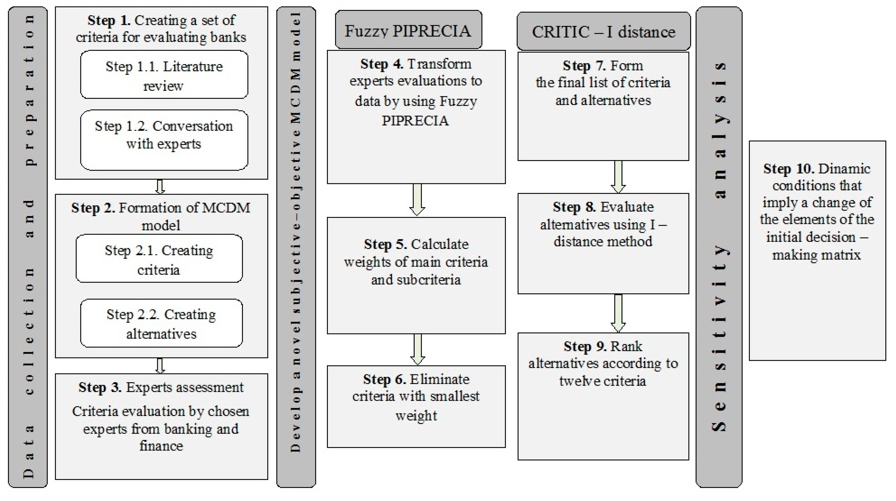
Figure 1 shows the proposed methodology consisting of three phases and a total of ten steps.
Creating a subjective-objective model for multi-criteria ranking of the alternatives required certain activities divided into three phases. Each phase involved a number of steps, and their importance was equally essential for the proper formation of the model. The initial phase, which related to data collection and preparation, as a first step involved the acquaintance with the most important literature and achievements in the field of MCDM. As part of that step, it was necessary to address all the significant studies conducted in the field of ranking business entities so far, and thus banks too. Since the model entailed consulting experts in one of its segments and accepting their preferences regarding various aspects (criteria) of bank performance, the second step involved careful selection of the criteria and consulting in relation to the selection of criteria and sub-criteria. The selection of criteria and alternatives was the following step, and within it, the angles from which the quality of a business entity would be viewed were determined. As banks represent one of the most important segments of both society and economy, and as bearers of stable and sustainable economic growth, they have been selected as alternatives in this MCDM model. The last step in that phase required the selected experts to evaluate the criteria and sub-criteria on the basis of their preferences, in order to further determine the significance of each of them individually.
The second phase had two of the most significant processes involved in the application of Fuzzy PIPRECIA, CRITIC and I-distance method. The first was to determine the weight coefficients for each of the main criteria and sub-criteria, and thus the first step in that phase was to convert expert preferences into numerical indicators, then the next step involved calculating the weights of all criteria, and the last step concerned the elimination of the least significant sub-criteria within the main criteria. The second part of the phase considered the application of I-distance and, within three steps, the final list of criteria and alternatives was formed. Then, it included the calculation of the values of I-distance according to the order based on the weights of criteria and the ranking of the alternatives in accordance with each of the main criteria, as well as a comprehensive ranking list of the alternatives observed. The last, third, phase involved the application of a sensitivity analysis within which a reverse rank matrix was calculated. The procedure tested the sensitivity of the final results to eliminating the lowest-ranked alternative from the set of observed alternatives.
3.1. Fuzzy PIvot Pairwise RElative Criteria Importance Assessment—Fuzzy PIPRECIA Method
The PIPRECIA method has some advantages in comparing to other methods, for example, in comparison to SWARA [
29,
30]. PIPRECIA accept that criteria be evaluated without their previously sorting by significance. Also, the benefits of fuzzy PIPRECIA are that on good way can solve MCDM problem with a large number of decision-makers (DMs) involved in the assessment of criteria. The Fuzzy PIPRECIA method was developed by Stević et al. [
31]. It consists of 11 steps shown below.
Step 1. Forming multi-criteria decision-making model including set of criteria and team of decision-makers.
Step 2. In order to determine the relative importance
sj of criterion
j (
Cj) in relation to the previous
j − 1 (
Cj−1), each DM evaluates criteria by starting from the second criterion, Equation (1).
where
denotes the evaluation of the criteria by a DM
r.To obtain a matrix
, there is need to perform the averaging of matrix
using a geometric or average mean. DMs evaluate the criteria using the linguistic scales developed and defined in [
31].
Step 3. Determining the coefficient
Step 4. Determining the fuzzy weight
Step 5. Determining the relative weight of the criterion
In the following steps, it is necessary to apply the inverse methodology of the fuzzy PIPRECIA method.
Step 6. Evaluation of the applying scale defined above, but this time starting from a penultimate criterion.
where
denotes the evaluation of the criteria by a DM
r.It is again necessary to average the matrix .
Step 7. Determining the coefficient
where
n denotes a total number of criteria. It means that the value of the last criterion is equal to (1, 1, 1).
Step 8. Determining the fuzzy weight
Step 9. Determining the relative weight of the criterion
Step 10. Determination of the final weights of the criteria.
Step 11. Control the obtained results using Spearman and Pearson correlation coefficients.
3.2. CRiteria Importance through Intercriteria Correlation—CRITIC Method
In DM problems, criteria, as a source of information, possess a weight which reflects the amount of the information contained in each of them. This weight is referred to as “objective weight”. Diakoulaki et al. [
32] introduced the CRITIC method for determining the objective weights of criteria in MCDM problems based on principles by using contrast intensity of each measure, considered as standard deviation, and conflict between criteria, regarded as the correlation coefficient between criteria [
33].
The following steps describe the CRITIC method. It is assumed that there is a set of n feasible alternatives Ai (i = 1, 2, …, n) and m evaluation criteria Cj (j = 1, 2, …, m).
Step 1. Forming of the decision matrix
X, expressed as follows.
The elements xij of the decision matrix (X) represent the performance value of ith alternative for jth criterion.
Step 2. Normalization of original decision matrix using the following equations for benefit criteria:
Step 3: Calculation of symmetric linear correlation matrix mij:
Step 4: Determination of the objective weight of a criterion using Equation (13).
where
Cj is the quantity of information contained in the criterion
j and is determined as follows:
where σ is the standard deviation of
jth criterion and the correlation coefficient between the two tests.
3.3. I-Distance Method
In this paper, we have decided to apply the I-distance method as one of the most complete methods that measures the distance between units of the basic set. Namely, this method respects the fact that the indicators do not have the same importance, and also they are interdependent wherefore there is some duplication of information in the ranking process. Due to the application of partial correlation coefficients in the calculation process (which will be explained later in this section), this method prevents duplication of information contained in multiple indicators, but also values their individual importance by determining the order in which the indicators are introduced into the analysis. The I-distance method was originally introduced and defined in the publications of Professor Branislav Ivanovic in the 1960s and 1970s. Professor Ivanovic designed the method to rank countries by the level of development, which he described by various socio-economic indicators. Using this method, one can determine the relative position of a unit in relation to the other, within the units of the dataset. Linear (clustered and non-clustered) and quadratic distance were worked out in the method, and further research in this field led to the development of a multi-stage I-distance, which will be used in this paper [
34,
35,
36].
The process of construction of I-distance is iterative, and the number of iterations depends on the number of indicators to be included in the analysis. If we observe a set of indicators
, which in this case describe quality of a certain field of operations, I-distance between the two observed units (banks)
and
is calculated on the basis of the following form [
35]:
where:
- -
is the distance between units er and es for indicator Ci;
- -
is standard deviation for the value of all units per indicator Ci;
- -
represents a partial correlation coefficient between indicators
Ci and
Cj [
37].
It was pointed out that the calculation of I-distance is a procedure which consists of several iterations. The process first involves the entire discriminatory effect of indicator
C1 or the indicator that has the most information about the level of “quality” of the unit. After that, the part of the discriminatory effect of the second indicator, which was not involved in the discriminatory effect of the first indicators, is added. Similar to the previous, the part of the information that provides the third indicator is added, which was not involved in the discriminatory effect of the first two. The whole process is continuing, so that, finally, the level of “quality” of the unit
ej defined by a set of indicator
C, could be:
If there are different signs of variables, resulting in the occurrence of negative correlation coefficient between the variables, it is necessary to use the square I-distance in the analysis [
35]. The involvement of indicators with less information is bigger in the square than in the plain distance, which is another reason to use square I-distance when we have a large number of indicators. The square I-distance is calculated as follows:
Bank ranking in this paper will be carried out by the use of the square I-distance, because of the occurrence of negative partial correlation coefficients between the observed indicators for ranking, but it is necessary to say that, due to the specific problem being solved, two-stage method of I-distance will be applied. This method involves calculating I-distance for units in the set in several stages, in this case in two stages. We will get to the results of I-distance within each segment and measurement of bank’s performance (liquidity, profitability, efficiency, solvency), and after that, we will again apply the same method to the obtained results in order to get the final bank ranking in the RS. This method will allow us to determine the best-performing banks for each of these segments, and the most successful one [
36,
38].
4. Results
4.1. Forming the MCDM Model
For the purpose of this paper, the RS banking sector, where currently operates eight banks with a dominant share of foreign capital, has been analyzed. Their business performance was measured throughout four the most significant aspects of banks’ performance, which also represented the ranking criteria: liquidity, efficiency, profitability and solvency. The indicators used for each of the performance criteria are listed and explained below, and which represented the sub-criteria in further analysis.
Liquidity of the bank is a complex concept, usually interpreted as bank’s ability to meet its obligations on maturity. The bank’s management is required to continuously monitor liquidity from the static and dynamic aspect. By disrupting the liquidity of only one bank, the survival of the entire financial system can be brought into question. If a bank is unable to service its obligations, general confidence in the financial system is lost and this leads to erosion of monetary assets of all banks. The following indicators are used in theory and practice to assess liquidity [
39]:
L1 = Cash and pledged marketable securities/Business assets,
L2 = Total deposits/Borrowings,
L3 = Variable funds/Liquid assets,
L4 = Total loans/Total deposits,
L5 = Liquid assets/Operating assets.
During the bank’s liquidity management, the indicators L1, L2, and L5 need to be maximized, i.e., higher value of these ratios shows better liquidity. Indicators L3 and L4 have completely opposite meaning, the low value of these indicators implicates that there is high liquidity, and vice versa. When analyzing the bank, it should not be forgotten that too high liquidity causes low profitability.
Efficiency is defined by the phrase “do things right”, and in a specific case it indicates that banks must manage their assets with the best possible strategy. A bank’s efficiency is achieved when the bank produces larger effects with as low as possible costs, increasing productive assets by placing liabilities in the best way under current circumstances [
39]. Productive assets bring interest income, the banks then increase capital, provided that they achieved positive financial results. The indicators that provide information on the effectiveness are:
E1 = Interest expense/Interest income,
E2 = Provisions/Net interest income,
E
3 = Interest income/Total number of employees [
40].
The data for this calculation is taken from the income statement and banks tend to minimize indicators E1 and E2—lower value rejects greater efficiency and vice versa. The indicator E3 has an alternative explanation, as the maximum value increases efficiency.
Profitability indicators are crucial for business analysis and are defined as the bank’s earning ability, or its ability to receive income of the invested assets and increase them during the business cycles. They are used for evaluation of the bank’s profitability in given time, usually at the end of the accounting period [
41]:
P1 = Profit before tax/Equity,
P2 = Profit before tax/Business assets,
P3 = Profit before tax/Interest income.
Higher values of profitability indicators signal a greater earning power and thus there is possibility of increasing the share capital. Caution should be exercised when interpreting the profitability indicators because numbers can distort the true picture. The profitability indicators are maximized, but as a result of the increase in net profit before tax, and not under the influence of the reduction of capital, assets or income from interest and the like.
Solvency or capital adequacy of a bank is an indicator to which we should pay more attention in the banking practice. To support this indicator, there is the statutory rate of minimum capital adequacy ratio of 12% and it represents the bank’s ability to fulfill all its obligations eventually, even from the bankruptcy estate. “A bank is considered insolvent when its liabilities exceed the value of its assets or when realized losses exceed its equity capital”. In that case, the bank does not have enough capital to cover the incurred losses, and a part of the assets are non-performing loans, receivables, loans, and there is no possibility to fulfill all its obligations [
39,
42]. The criteria used to test the solvency (adequacy) of the bank are:
S1 = Total Liabilities/Equity;
S2 = Total deposits/Equity;
S3 = Venture capital/Total risk-weighted assets;
S4 = Shareholders’ equity/Business assets;
S5 = Shareholders’ equity/Risk-weighted assets;
S6 = Shareholders’ equity/Total deposits;
S7 = Shareholders’ equity/Loans.
When managing solvency, the bank should tend to minimize the indicators S1 and S2 and make the other indicators as large as possible. Instead of total assets and total resources, operating assets and business assets are included in the calculation of these indicators. Banks are for-profit organizations and business assets, which represent the funds arising from operations, participate directly in making a profit and are fully justifiably included in the calculation. Confirmation of this is that the total assets represent the sum of operating assets and off-balance assets, where the off- balance sheet are sureties, guarantees, acceptances, bills of exchange and other forms of guarantees, uncovered letters of credit, irrevocable, approved but undrawn loans and the like. A characteristic of off-balance sheet positions is that they are potential liabilities or claims and that there is some uncertainty whether and when those contingent liabilities and receivables would be implemented. Banks often use off-balance sheet transactions in order to earn additional income accomplished through commission fees. To conclude, off-balance sheet (assets) are excluded from the calculation because the aim of the research is to show the real rank and position of the banks in the RS banking sector on the basis of their core business.
The criteria and sub-criteria described above were evaluated by banking experts and they were assigned certain significance according to experts’ preferences. The expert team included in the analysis was comprised of experts with years of experience in banking, finance, accounting and auditing. The team involved five experts, one of whom is a university professor with 25 years of experience in bank management, then a university professor with 20 years of experience in accounting and auditing, and with a title of a certified accountant and auditor. In addition, the team consisted of two members with over 10 years of experience working at senior banking positions, primarily in corporate banking. Additionally, as a member of the team and one of the experts who evaluated the significance of the criteria was a person with many years of experience in the field of auditing, and currently employed at one of the four leading auditing companies in the world.
Considering that the model was based on measuring the performance of banks and that the above criteria aimed to measure the quality of each individual segment of bank operations in the best possible way, it is logical that banks operating in the market of the Republic of Srpska were taken as alternatives. The performance indicators of the banks referred to 2018 and data were taken from the official financial and audit reports.
Table 1 shows the quantitatively expressed values of indicators for observed banks in 2018.
4.2. The Evaluation of Criteria Using the Fuzzy PIPRECIA Method
The evaluation of the criteria has been performed using a linguistic scale that involves quantification into fuzzy triangular numbers.
Table 2 shows the evaluation of the criteria for fuzzy PIPRECIA and inverse fuzzy PIPRECIA by decision-makers and the average values (AV) which are used for further calculation. It is important to note that, compared to the original method developed in [
31], the average value (AV) is used here to average decision-makers’ preferences, which in this specific case contributed to the more accurate input parameters of the model. Whether a geometric mean or an average value is applied depends directly on a particular case. Both methods of averaging are valid.
Based on the evaluation of the criteria and their averaging, Equation (1), a matrix
sj is formed.
Using Equation (2), those values are subtracted from number two. Following the rules of operations with fuzzy numbers, the
kj matrix
is obtained as follows:
According to Equation (2), the value
Applying Equation (3), the value
qj
is obtained as follows:
Applying Equation (4), the relative weights are calculated:
For determining the final weights of the criteria Equations (5)–(9) or the methodology of the inverse fuzzy PIPRECIA method are applied. Based on the evaluation by the DMs and the application of the average value, the matrix
sj’ is obtained.
Applying Equation (6), the values of matrix
kj’ are obtained:
Applying Equation (7), the following values are obtained:
After that, it is necessary to apply Equation (8) to obtain relative weights for the fuzzy Inverse PIPRECIA method.
The results of the applied methodology are presented in
Table 3. These results refer only to the calculation of the main criteria: liquidity, efficiency, profitability and capital adequacy. The weights for all sub-criteria across all levels of the hierarchy are calculated in the same way.
Using Equation (9), the final weights of the main criteria are obtained. Before using this equation, it is necessary to defuzzify the values of the criteria.
Table 3 shows the complete previous calculation, and the last column shows the defuzzified values of the relative weights of the criteria.
Figure 2 shows the final result of the procedure for determining the individual significance of each of the main criteria. As explained above, based on the personal preferences of the experts, the significance of the observed criteria was obtained using the Fuzzy PIPRECIA method, and they are the “blue” values in
Figure 2. Then, the defuzzification of the values was carried out to obtain the final weights of all the main criteria. The weights are marked in gray, and based on them we can determine that the most significant criterion is C
3 (profitability) with a weight coefficient of 0.295, followed by C
4 (solvency or capital adequacy) with a weight of 0.282, and C
1 (liquidity) with 0.226 and finally C2 (efficiency) with a weight of 0.215. This procedure is of great importance in further analysis since it determines the order of introducing the main criteria into the procedure to calculate the I-distance.
Spearman’s correlation coefficient for the ranks obtained with fuzzy PIPRECIA and Inverse fuzzy PIPRECIA is 1.00, which means that these ranks are in complete correlation. Additionally, Pearson’s correlation coefficient has been calculated for the weights of the criteria obtained using these approaches and is 0.966. In the same manner as previously shown, the values of all sub-criteria have been obtained, as shown in
Table 4,
Table 5,
Table 6 and
Table 7.
Spearman’s correlation coefficient for the ranks obtained within the liquidity group is 1.00, which means that these ranks are in complete correlation. Pearson’s correlation coefficient for the weights of the criteria, which is 0.938, has also been calculated.
Spearman’s correlation coefficient for the ranks obtained within the efficiency group is also 1.00, while Pearson’s correlation coefficient for the weights of the criteria is 0.987.
Spearman and Pearson correlation coefficients for the ranks obtained within the profitability group are 1.00.
Spearman’s correlation coefficient for the ranks obtained within the capital adequacy group is 1.00, which means that these ranks are in complete correlation. Pearson’s correlation coefficient for the weights of the criteria, which is 0.984, has also been calculated.
The final weights of the criteria were created as the product of the main criterion weights and the values of the weights obtained within individual groups.
Table 8 presents the final weight results using the fuzzy PIPRECIA method. Since there are four sets of criteria that include a total of 18 sub-criteria not distributed equally across the groups, a further calculation is made in order to obtain as accurate results as possible. This is demonstrated through the following subsection, which outlines the way in which the formation of a hierarchical structure influences the weights of the criteria.
4.3. The Influence of Hierarchical Structure on Determining the Values of Criteria
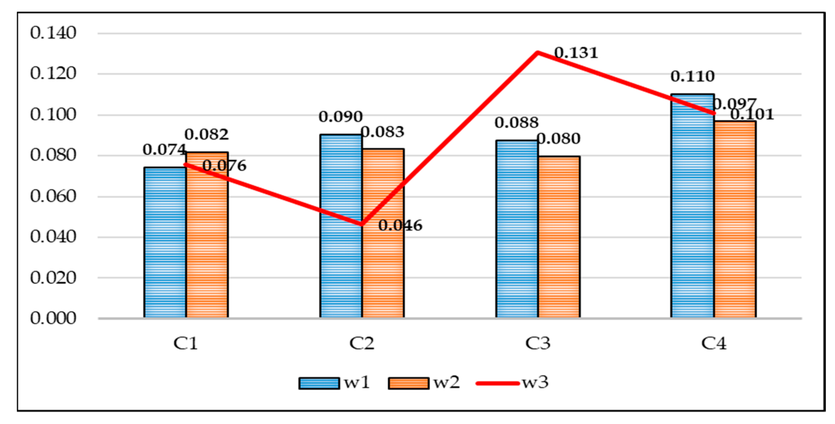
The purpose of this subsection is to point out that there is a huge influence of the hierarchical structure on obtaining the final values of criteria. Namely, in most studies, if evaluation is made on the basis of more than nine criteria, the levels arranged in a hierarchical structure are formed, as is the case in this paper. However, if the criteria at the first level have a different number of sub-criteria at the second level, there is a problem of giving preference to certain criteria that do not really deserve it. In this way, results obtained depend directly on the number of sub-criteria in each group, rather than on the actual preferences of decision-makers. We will take a simple example where the weights of all the criteria and sub-criteria are equal in order to demonstrate the problem as clearly as possible and make a proposal for its solution.
Example: Suppose we have four main criteria at the first level of the hierarchy and each of them has a different number of sub-criteria. The first criterion has five sub-criteria, the second criterion has three sub-criteria, the third criterion has four sub-criteria and the fourth has six sub-criteria. As stated, all have equal importance, meaning that the value of each main criterion is w1 = w2 = w3 = w4 = 0.250 in order that the sum of them is one. If the value of all sub-criteria is also equal within individual groups, the results will be as presented in
Table 9.
If all the criteria are equally important, then the values of each sub-criterion should be identical. If we observe the same example, the value of each criterion should be 0.55, which, we notice, is not the case. The sub-criteria of the second group are of the highest value, since there is the smallest number of them, which means that the hierarchical structure formed in this way does not allow objective results and weights of the criteria. If it is taken into account that in almost all cases the criteria have comparative significance that differs among the criteria, i.e., the main criteria have different values, then the influence of the sub-criteria of the group with the smallest number of elements is even greater. Thus, certain criteria undeservedly gain great values and have a greater impact on the final decision than they really should.
Since, in this paper, a hierarchical structure was formed with an unequal number of elements within different groups, in order to obtain adequate and realistic values of the criteria for the evaluation of alternatives, their selection was made. Within each group of the criteria, three of the most important were selected, so that 12 out of 18 criteria were included in further calculation. In order to maintain the constraint that the sum of all criteria is equal to one, the following equation was applied:
where
wm denotes the criteria remaining in the model and
wn denotes the criteria exiting the model.
n is the total number of criteria exiting the model and
m is the total number of criteria remaining in the model.
In order to obtain the values of the 12 criteria that are equally represented in the hierarchical structure (
Figure 3), the values of the criteria exiting the model are equally distributed to the criteria that remain in the model by applying Equation (18). Since the efficiency group and profitability group have per three sub-criteria from the beginning, they have been unchanged. For the liquidity group, the procedure for obtaining the weights of the criteria is as follows.
while for the capital adequacy group is as follows:
In order to ensure objectivity in determining the significance of the criteria, as a support to the subjective fuzzy PIPRECIA method, the weights of the criteria were also calculated using the objective CRITIC method. Then, averaging by the average weight, the final weight values of the criteria and their ranks, which represented the input parameters for ranking alternatives using the I-distance method, were obtained. The outcomes of the previous analysis are the weights of all criteria and sub-criteria, but also the basis for the elimination of certain less important criteria. Accordingly, only the main criteria with per three sub-criteria were retained in the further analysis. The sub-criteria L1 and L2 (marked as C11 and C12 in the analysis) were eliminated from further consideration within the liquidity criteria since their weight coefficients were shown to be the lowest within the main criterion. Similarly, the sub-criteria S1, S2, S3 and S4 were eliminated from the main solvency (capital adequacy) criterion (marked as C41, C42, C43 and C44 in the analysis). Within the efficiency and profitability criteria, there was no need to eliminate the criteria since they had already contained per three sub-criteria, and thus the hierarchical structure was not disrupted.
4.4. Determining the Significance of the Criteria Using the CRITIC Method
The objective CRITIC method for obtaining the weights of the criteria uses the initial matrix of the multi-criteria model, which is shown in
Table 10.
After that, it is required to perform normalization by applying Equations (11) and (12) as in the case of normalization in the MABAC method [
43,
44,
45]. The normalized matrix with the calculated standard deviation is shown in
Table 11.
After normalizing the matrix and calculating the standard deviation, it is necessary to determine the correlation among the criteria, which is shown in
Table 12. Essentially, a 12 × 12 symmetric matrix is obtained.
Subtracting the elements of the correlation matrix from number one, then summing these values, a matrix 1 × 12 is created, after which the summed values are multiplied by the standard deviation and a matrix
cj is obtained. Simply summing these values and dividing the individual elements by the sum yields the final criterion values using the CRITIC method.
4.5. Determination of the Final Values of the Criteria by Applying an Integrated Subjective-Objective Model
Based on all previous calculations and the implementation of the integrated model, the final values of the criteria (
Table 13), which are further used to evaluate the alternatives, are obtained.
As shown in
Table 13, 12 sub-criteria were retained in the further analysis, per three within each main criterion. The calculated weight coefficients determined the order of introducing the criteria and sub-criteria in the further analysis and calculation of the values by applying the I-distance. The values in the table indicate that the weights of the individual sub-criteria are fairly uniform and range from 0.062 to 0.100.
4.6. Evaluation of the Alternatives by Applying I-Distance Method
In this paper, the ranking of banks is performed by applying the square I-distance due to the appearance of negative partial correlation coefficients among the observed ranking indicators, but it is also necessary to say that due to the specificity of the problem, the two-stage I-distance method will be applied. The method involves calculating the I-distance for the units of a set in several stages, in this particular case in two stages. Namely, the results of I-distance within each of the segments of observing and measuring banks’ performance (liquidity, profitability, efficiency, solvency) will be obtained first, and then the same method will be applied again to already obtained results in order to reach the final ranking of the banks in the RS. The method will allow us to determine which banks are the most successful in each of the above segments, but also which of them is the most successful bank overall [
46].
The order of introducing the criteria, determined by their weights, was as follows: the profitability criterion was first introduced into the analysis, and within the criterion the order of introduction of the sub-criterion was C33, then C31, and finally C32. The next criterion of importance was solvency, whose sub-criterion C41 was first introduced, followed by C43 and last C42. After solvency, the criterion of liquidity was introduced into the analysis, and the significance and order of the sub-criteria was as follows: C12, C13 and finally C11. The last in terms of importance was the efficiency criterion, whose sub-criteria were introduced in the following order: C22, C21 and finally C23.
Before analyzing the results, for a better understanding of the calculation of I-distance method, the value for alternative A
1 for indicator C
1 was calculated:
The order of introducing the criteria and sub-criteria has been explained previously, and accordingly this calculation refers to the profitability criterion and its corresponding sub-criteria. The same method of calculation has been applied for other criteria and sub-criteria, and the final values of I-distance used for ranking are given in the following section of the paper.
All of the above-described methods aimed to enable the ranking of the observed alternatives (banks) and to show the quality of each observed unit in relation to others. Data on the quality of alternatives within each of the main criteria observed, as well as overall, are presented in
Table 14.
The data in the table shows the results by each of the main criteria, as well as the final ranking of banks’ performance in 2018. According to the first and most important criterion, the results indicate that the most profitable bank in the RS was NLB Bank, followed by Unicredit Bank, and Komercijalna Bank in the third place. The lowest-ranked bank by the criterion was Pavlovic Bank, which achieved the worst results by all sub-criteria. The next analyzed criterion was solvency and the results showed that Hypo Bank was the best-ranked bank, followed by Komercijalna and Pavlovic Bank. The lowest-ranked banks according to this criterion were MF and NLB bank. The third criterion in terms of importance was liquidity, and within it, the results showed that Sberbank, followed by MF and Pavlovic Bank had the best liquidity. The last-ranked bank according to this criterion was Komercijalna Bank, with much lower liquidity than other banks. The last criterion by which banks are ranked was efficiency and the most efficient was Unicredit Bank, followed by MF and NLB Bank. The worst efficiency of all banks had Pavlovic Bank. Based on the ranking results obtained by each of the criteria, the final ranking of banks’ performance was obtained and the most successful bank in the RS in 2018 was Unicredit Bank, followed by NLB and Hypo Bank, while Komercijalna and MF Bank took the fourth and fifth place with a slight difference. In terms of performance, Sberbank was after them, followed by Nova Bank. By far, Pavlovic Bank was in the last place.
5. Sensitivity Analysis and Discussion
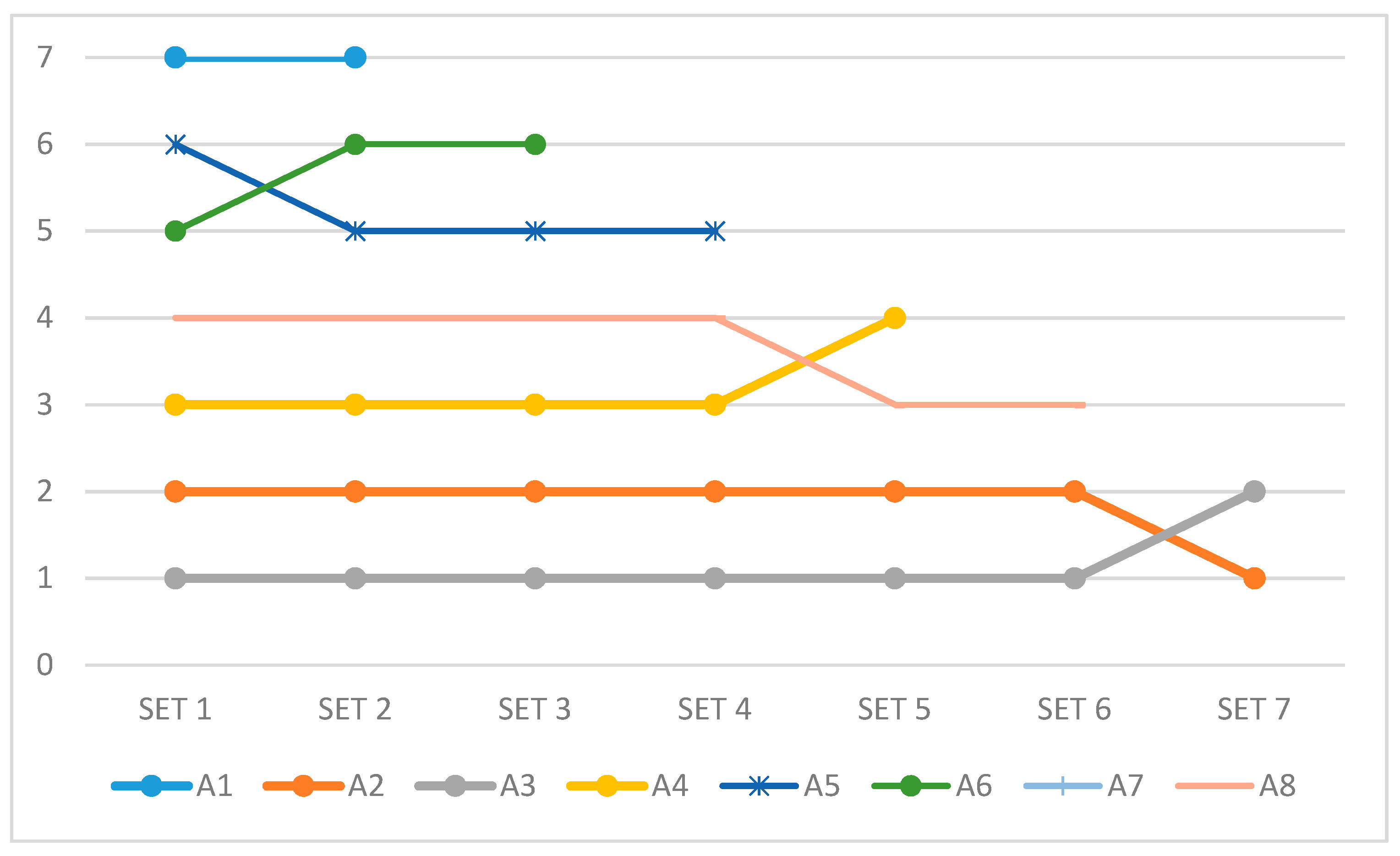
As part of the sensitivity analysis (SA), the dynamic impact on the rankings of the alternatives was checked, as shown in
Figure 4.
Modification certain elements of the MCDM matrix, like introducing a new or eliminating the existing alternative, can be influenced by changes in preferences. Therefore, several scenarios are created in which the modification of the elements of MCDM matrix is simulated. In all scenarios, a modification in the number of alternatives is performed, after which in such conditions the model is applied. Scenarios are created in a way that in each scenario the worst option is removed from consideration. After that model is applied taking into account new decision-making matrix. This part of SA has an objective: the analysis of the output of the proposed model in dynamic conditions. The obtained results applying the novel subjective-objective model is generated as A3 > A2 > A4 > A8 > A6 > A5 > A1 > A7. Alternative A7 is the worst, so in the first scenario it is removed. Thus, a new initial matrix is created with a total of seven alternatives. A new solution is generated, and the following results are obtained: A3 > A2 > A4 > A8 > A5 > A6 > A1. The results from the first scenario show that A3 remains the best alternative, while A1 remains the worst alternative. In this set, only A5 and A6 replace their positions. The subsequent scenario involves the elimination of alternative A1, as the worst, and the result is as follows: A3 > A2 > A4 > A8 > A5 > A6. Based on these preferences, it is concluded that no alternative has changed its ranking compared to the previous scenario. Subsequently, alternative A6 is eliminated from the analysis, as the worst. In the further analysis, five alternatives remain, and the preferences are completely the same in relation to the previous scenario: A3 > A2 > A4 > A8 > A5. It is continued with the elimination of the worst-ranked alternatives, and then the analysis with only four remaining alternatives is performed since A5 has been eliminated. Their ranking is as follows: A3 > A2 > A4 > A8. In this step, alternatives A4 and A8 have switched their placed and alternative A8 becomes the worst ranked. Accordingly, in the next step, it is eliminated, and the new order of the remaining three alternatives remain unchanged comparing to the previous step: A3 > A2 >A4. In the last step, only alternatives A3 and A2 remain, and in their mutual comparison, alternative A2 is described as better.
Based on this analysis, we can conclude that eliminating the last-ranked alternative has not resulted in a significant change in the final order of alternatives. Alternatives A5 and A6 and alternatives A4 and A8 have switched their places but observing the original ranking list and the values of I-distance, we can conclude that the differences between these alternatives are almost negligible (10.017 > 9.939 and 12.508 > 12.364, respectively). The change between alternatives A3 and A2 is due to the order of introducing the criteria into the calculation of I-distance, in which the discriminatory effect of the first-introduced criterion is fully evaluated, while the others are reduced proportionally to the partial correlation coefficients (explained in the section related to the I-distance method).
The concept of this paper implied that individual preferences of experts in specific fields were merged with the objective methods of multi-criteria decision-making in one model. Their preferences were transformed into numerical indicators throughout various mathematical transformations that determined the significance of each of the four main criteria on the basis of which they were further introduced into the analysis. The area of interest in this paper was the RS banking sector and the research conducted included eight banks with headquarters in the RS. Although most economists when considering the aspects of bank performance take solvency as the most important, new studies and views of experts have confirmed that profitability is more important than solvency now since good profitability also guarantees good solvency. It is important to emphasize that the differences in the significance of the four main criteria, according to experts, were extremely small. The most significant criterion (profitability) had a weight coefficient of 0.295, while the weight coefficient of the least significant (efficiency) was 0.215. After the formation of the hierarchical structure, the elimination of certain sub-criteria was performed in order to obtain the same number of sub-criteria within each main criterion. This segment is extremely important since it contributes to the equalization of the importance of each individual sub-criterion, i.e., allows no criterion to be in a subordinate position in further analysis. Subsequently, using the two-stage method of square I-distance, the calculations were made and the final ranking lists of alternatives (banks) were obtained according to each of the main criteria, as well as a comprehensive ranking list. The results show that banks which have a long tradition and operate in several European countries have the best results in this ranking. If average values are taken as a certain threshold of success, it is noted that only four banks are above the threshold in terms of profitability. Within this main criterion, it can be said that Nova Bank, Hypo Bank, Sberbank, and Pavlovic Bank are below the level considered as the lower profitability limit. When it comes to solvency, only three banks again have higher average solvency than, in this case, Hypo, Komercijalna, and Pavlovic Bank. The next observed criterion is liquidity, and within it, four banks have higher-than-average values, namely Sberbank, MF Bank, Hypo Bank, and Pavlovic Bank. The last analyzed main criterion is efficiency and it is concluded that only Unicredit and MF bank are above average within the criterion. It is important to note that within this criterion, Unicredit Bank drastically differs from the rest, which is the result of high-quality placements affecting the low cost of provisions. In addition, high-quality sources of capital allow them to have the ratio of costs and interest income almost seven times on the revenue side.
6. Conclusions
In this paper, a novel integrated subjective–objective methodology for solving MCDM problems has been created. Through its development, one of the main contributions of the paper, which enrich the area of addressing multi-criteria problems, has been presented. In addition, a brief critique of previous MCDM problems with an unbalanced hierarchical structure at the lower levels of the hierarchy has been made, which practically has a great influence on the final decision-making, i.e., determining the weights of criteria. This is explained and proved through a specific example. The foregoing reflects the scientific contribution of the study. In addition, the expert contribution of the research refers to the application of the developed multi-criteria model that enables the ranking of banks as economic units, based on the most significant indicators of their business performance.
One of the main ideas of this paper is to form a comprehensive model that will accept the subjective views and preferences of experts, as well as objective methods that address multi-criteria decision-making. The reasons for this approach lie in the fact that the symbiosis of the two approaches can produce more accurate results applicable in various situations and available to decision-makers at all levels. This model answers several questions: when it comes to the hierarchical structure of the observed criteria, it answers the question of their significance, then it balances their importance and does not allow any significant preference for any particular criterion or sub-criterion. The results of applying this model have been market-verified, too. Namely, as the data are from 2018, the worst-ranked bank, Pavlovic Bank, got into significant problems in 2019 and during the year it had to make a significant recapitalization and even change its ownership, and thus the management structures. The model has ranked Unicredit and NLB as the best banks, which are certainly the most stable players in the banking market, both in the RS and B&H and at European level. These are banks with firm sources of capital, for which they do not pay high interest costs, and considering the market where they are, they are able to generate significant interest income and thus show exceptional results in terms of profitability and efficiency. The results of the model would be even more significant if the selected indicators were monitored in the period shorter than one year and if the changes and possible improvements or deterioration of certain banks’ performance could be monitored. All the above is in favor of the accuracy and applicability of the model, not only to banks, but also to other economic units (enterprises, insurance companies, local governments, etc.), whose business performance can be measured by different quality indicators.
Future research may adopt several different directions. Considering that every business, and especially in the domain of banking, is market dynamic and subject to change, this model should adapt to new trends and challenges in banking in the future. This primarily refers to research in the field of indicators, expansion of existing ones or introduction of new ones, as well as constant consulting with experts in the field regarding the identification of certain changes in significance of the criteria. New times bring new challenges for all business units, and therefore opportunities for changes in the importance of particular aspects of business excellence, which certainly requires a permanent alignment of the subjective segment of the model. In addition, further research refers to the further integration of uncertainty theory, such as fuzzy logic, rough sets, with other approaches, and the integration of subjective–objective models in order to achieve more accurate and approximately optimal results.


 ,
, 


