Micromagnetorotation of MHD Micropolar Flows

Abstract

The studies dealing with micropolar magnetohydrodynamic (MHD) flows usually ignore the micromagnetorotation (MMR) effect, by assuming that magnetization and magnetic field vectors are parallel. The main objective of the present investigation is to measure the effect of MMR and the possible differences encountered by ignoring it. The MHD planar Couette micropolar flow is solved analytically considering and by ignoring the MMR effect. Subsequently, the influence of MMR on the velocity and microrotation fields as well as skin friction coefficient, is evaluated for various micropolar size and electric effect parameters and Hartmann numbers. It is concluded that depending on the parameters’ combination, as MMR varies, the fluid flow may accelerate, decelerate, or even excite a mixed pattern along the channel height. Thus, the MMR term is a side mechanism, other than the Lorentz force, that transfers or dissipates magnetic energy in the flow direct through microrotation. Acceleration or deceleration of the velocity from 4% to even up to 45% and almost 15% deviation of the skin friction were measured when MMR was considered. The crucial effect of the micromagnetorotation term, which is usually ignored, should be considered for the future design of industrial and bioengineering applications.

1. Introduction

The model of micropolar fluids proposed by Eringen [1,2] is a mathematical theory, which accounts also for the local microstructure of a fluid. It is considered as a generalization of the well-known Newtonian model, which assumes that the fluid particles have no internal characteristics [3,4]. The micropolar theory describes fluids with a wide variety of microstructure by assuming that their internal particles may rotate independent of their linear velocity [5,6]. Furthermore, micropolar fluids are viscous fluids with a non-symmetric stress tensor [7]. Consequently, a new equation is added, which is formulated by the balance law of angular momentum, while a new vector field (the microrotation) is introduced, which describes the total angular velocity of the suspended fluid’s particles. Some examples of fluids which can be described by the micropolar theory are liquid crystals [8], lubricants [9,10], ferrofluids [11], water [12], and granular flows [13,14].

Magnetohydrodynamics (MHD) is the science that deals with the flow of electrically conducting fluids in the presence of a magnetic field. The motion of the conducting fluid across this magnetic field creates electric currents. The interaction of the magnetic field with these currents produces mechanical forces, known as Lorentz forces, which influence the flow of the fluid. Eringen [15,16] examined the magnetohydrodynamics as well as electrodynamics of micropolar fluids. The latter is the branch of physics that investigates phenomena related with moving charged bodies along with varying electric and magnetic fields, given that a magnetic field is developed by the moving charges. Since Eringen’s studies [15,16], a plethora of researchers have examined MHD micropolar flows. Chen et al. [17] established a set of equations for the electrodynamics of micropolar fluids utilizing the balance laws of mass, linear momentum, angular momentum, energy, and entropy for micropolar fluid dynamics integrated with Maxwell’s equations. Onsager’s theory and Wang’s representation theorem, which were based on the principle of objectivity, were incorporated for the constitutive equations. They also derived a linear formulation that can be used for magneto-micropolar fluid dynamics and plasma physics. Murthy et al. [18] investigated the steady flow of an incompressible conducting micropolar fluid through a rectangular channel in the presence of a transverse magnetic field. The induced magnetic and electric fields were negligible and the velocity with microrotation was obtained with the use of Fourier series. Moreover, the volumetric flow rate was calculated, while the microrotation parameter, geometric parameter and Hartmann number effects on the flow were investigated. Yadav et al. [19] studied the flow of a micropolar fluid between two Newtonian fluid layers through a horizontal porous channel. The flow was driven by a constant pressure gradient and a uniform magnetic field was applied in the direction perpendicular to the flow. The solution of the flow was obtained numerically, and the results were used for evaluating the influence of various transport parameters such as magnetic number, viscosity ratio on the velocity and microrotation profiles. Patel et al. [20] examined the mixed convection of a micropolar fluid in a porous medium in the presence of a uniform magnetic field for a nonlinear stretched surface by considering viscous dissipation and Joule heating. Further, heat and mass transfer were studied along with thermophoresis, Brownian motion, non-linear thermal radiation and chemical reaction. They concluded that the velocity profiles in case of linear stretching sheet were reduced compared to those of non-linear stretching sheet. In addition, the values of skin-friction coefficient were higher for the case of strong concentration in comparison with the case of weak concentration. Furthermore, Brownian motion and the thermophoresis parameter improved the heat transfer, whereas the mass transfer was reduced with the variation of the chemical reaction parameter.

A subclass of micropolar fluids is biological fluids, such as blood [21]. A plethora of researchers have used the micropolar continuum theory of Eringen to describe blood flow. Ariman [22] used the theory of micropolar fluids with stretch in order to analyze blood flow in relatively small arteries. No-slip conditions were imposed for the velocity boundary conditions and exact solutions of the governing equations were obtained. Mekheimer et al. [23] and Asadi et al. [24] established micropolar models for blood flows through tapered stenosed artery. As far as the investigation of blood flows subject to magnetic fields is concerned, Eringen’s MHD micropolar fluid model has widely been incorporated. Bhargava et al. [25] examined a two-dimensional fully developed steady-state, viscous hydrodynamic flow of a deoxygenated biomagnetic micropolar fluid. The solution of the problem was obtained numerically and the effect of various dimensionless parameters, such as biomagnetic number, was discussed on the velocity and microrotation profiles. Abdullah et al. [26] investigated the rheological properties of MHD blood flow via the constitutive equations of a micropolar fluid. The unsteady nonlinear differential system along with the corresponding boundary conditions was solved numerically and the results pertaining to the axial velocity, flow rate and wall shear stress were obtained. It was found that the applied magnetic field results in reduced blood flow rate. Recently, Jaiswal et al. [27] presented a two-fluid model of blood flow through a porous layered artery in the presence of a uniform magnetic field transversely applied to the direction of blood flow. Blood was assumed as a micropolar fluid in the core region and plasma is treated as a Newtonian fluid in a second region of the artery, which comprises 55% of blood volume [28]. Analytical solutions of the flow velocity, microrotation, flow rate and stresses at the wall through the composite porous walled artery were obtained. The effect of several flow parameters on the two-fluid model of blood flow was examined. They concluded that the different permeabilities of Darcy and Brinkman regions of the porous layered artery affects the flow.

As mentioned above, Eringen’s MHD model for micropolar fluids has been incorporated by several researchers for the purpose of investigating various micropolar MHD flows. This model was developed based on Maxwell’s equations and micropolar balance laws. However, in the balance law of the angular momentum the internal rotation because of the magnetization has not been included, since magnetization was considered parallel to the magnetic field. To this end, Shizawa et al. [29] obtained a set of equations for micropolar fluids with good thermal and electrical conductivity including internal rotation. In their context, magnetization does not depend only on thermodynamic quantities, but on the state of flow as well because of the anisotropy of magnetic fluids. Thus, magnetization vector was not assumed parallel to the magnetic field vector and thus micromagnetorotation (MMR) effects in microrotation are non-zero. Shizawa et al. [29] presented an analytical solution of the planar Couette micropolar flow with the MMR term, without however, emphasizing on the effect of the term in linear velocity and microrotation. Moreover, it appears that at most of the relevant literature where magnetization is considered, the MMR term is ignored in micropolar equations.

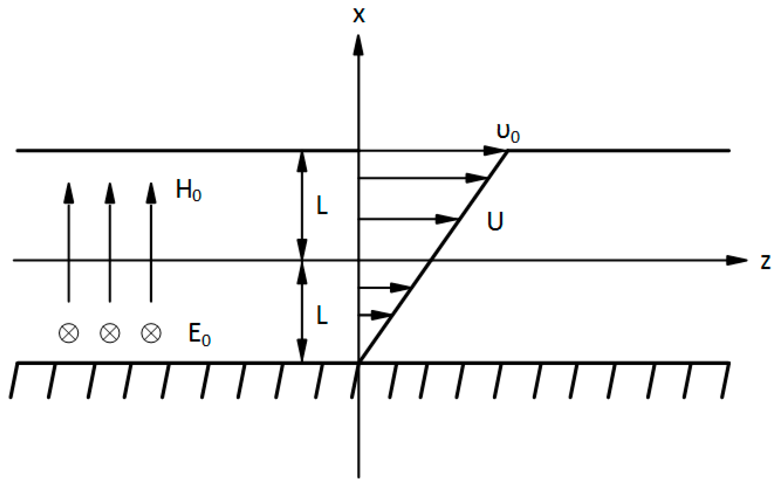
To the authors knowledge, there are extremely limited studies on micropolar flows considering that due to magnetization, MMR effect on microrotation [30,31] is important. In the present model flow, a simple micropolar Couette flow is examined under uniform magnetic and electric fields. The solutions of the dimensionless equations regarding velocity and microrotation are obtained analytically, using both Eringen’s MHD micropolar mathematical model [15,16] and MMR model of Shizawa-Tanahashi [29]. Consequently, the effects of various important dimensionless parameters entering the problem due to the MMR term on velocity and microrotation are discussed and useful conclusions are drawn. In the present investigation, an elaborate study is presented in order to capture the differences arising because of the MMR term. Hence, the limitations of ignoring the term are investigated, aiming at filling the gap of knowledge in the relative literature. The importance of this investigation is reinforced taking also into account the ongoing usage of magnetic fields in biological fluids, which are described as micropolar. The applications of this include magnetic targeted drug delivery systems [32], magnetic hyperthermia for thermal ablation of cancer cells [28], and lessening of bleeding in surgeries [33] to mention but a few.

2. Model and Governing Equations

2.1. Statement of the Problem

The flow of a micropolar fluid between two infinite parallel planes is considered in this investigation, as can be illustrated in Figure 1. The Cartesian coordinate system $\left(\overline{x}, \overline{y}, \overline{z}\right)$ is used to describe the physical plane. A constant electric field along with a constant magnetic field are applied with components, $\mathit{E}=\left(0,-E_0,0\right)$ and $\mathit{H}=\left(H_0,0, 0\right),$ respectively. The pressure gradient towards the $\overline{z}$ direction is considered to be zero $\left(\frac{\partial \overline{p}}{\partial \overline{z}}=0\right)$. The linear velocity component is given as $\mathit{U}=\left(0, 0,\overline{\upsilon } \left(\overline{x}\right)\right)$, the angular velocity of the fluid is given by $\mathit{w}=\left(0, \overline{\omega } \left(\overline{x}\right), 0\right)$ and the microrotational velocity component is given as $\mathit{W}=\left(0, \overline{\Omega } \left(\overline{x}\right), 0\right)$. The flow is free of external mechanical body forces, body couples and electric charges. Any temperature differences between the plates and polarization of the fluid are ignored. The upper and lower wall surfaces are insulators, i.e., ${\chi }_m\cong 0$, where ${\chi }_m$ is the magnetic susceptibility. The upper plane moves at constant velocity, ${\upsilon }_0$, and is located at $\overline{x}=L$ whereas the lower plane is still and located at $\overline{x}=-L$, where $L$ is the half-distance between the two planes. The following boundary conditions are imposed:

• No-slip and no-penetration conditions for the velocity field, i.e., ${\mathit{\upsilon }|}_{\overline{x}=-L}=0$ and ${\mathit{\upsilon }|}_{\overline{x}=L}={\upsilon }_0$.
• Condiff–Dahler conditions for the microrotation field and the angular velocity, i.e., $\mathit{W}=\delta \mathit{w}$, where $\delta$ is called wall coefficient. In this study $\delta =0$, which means that the microelements close to the wall are unable to rotate [34].

2.2. Governing Equations

A set of basic equations for nonconducting magnetic fluids with internal rotation and a set of basic equations for conducting magnetic fluids treated as a limit of nonpolar theory are combined. The system of equations concerning conducting fluids is extended within the limits of micropolar fluid theory using a thermodynamic method for both set of equations. Constitutive equations of stress tensor, couple stress tensor, and so on are calculated such that the second law of thermodynamics is satisfied, and dissipation function is positive based on kinematical balance equations. When internal rotation is considered, magnetization depends both on thermodynamic quantities and the state of flow because of anisotropy of magnetic fluids. Therefore, magnetization vector cannot be assumed parallel to the magnetic field vector. A constitutive equation of magnetization is introduced using a dissipation function instead of a relaxation equation, while magnetic susceptibility tensor is included. The complete set of equations is [29,30]:

$$\nabla ·\mathit{U}=0,$$

(1)

$$\nabla ·\mathit{W}=0,$$

(2)

$$\rho \frac{d\mathit{U}}{dt}=-\nabla \overline{p}+\eta ∆\mathit{U}+2{\eta }_1\nabla \times \left(\mathit{W}-\mathit{w}\right)+\mathit{j}\times \mathit{B}+\left(\mathit{M}·\nabla \right)\mathit{H}+\mathit{M}\times \left(\nabla \times \mathit{H}\right),$$

(3)

$$l\frac{d\mathit{W}}{dt}=\gamma ∆\mathit{W}+4{\eta }_1\nabla \times \left(\mathit{w}-\mathit{W}\right)+\mathit{M}\times \mathit{H}.$$

(4)

where $\rho$ is density, $t$ is time, $\overline{p}$ is pressure, $l$ is the moment of inertia, $\gamma$ is angular viscosity coefficient, $\eta$ is shear viscosity coefficient, and ${\eta }_1$ is vortex viscosity coefficient, $\mathit{M}$ is the magnetization vector, $\mathit{B}$ is the magnetic flux density vector, $\mathit{j}$ is the current density, and the MMR term is $\mathit{M}\times \mathit{H}$ in Equation (4). The angular velocity of the fluid is given by:

$$\mathit{w}=\nabla \times \frac{\mathit{U}}{2}.$$

(5)

The constitutive equations of the magnetization vector and magnetic flux density vector are given by:

$$\mathit{M}=\frac{M_0\left(\mathit{I}-\tau \mathit{\Omega }·\mathit{\epsilon }\right)·\mathit{H}}{H},$$

(6)

$$\mathit{B}={\mu }_0\mathit{H}+\mathit{M}.$$

(7)

where $M_0$ is the magnetization strength, $\mathit{I}$ is the identical tensor, $\mathit{\epsilon }$ is Levi-Civita’s symbol and ${\mu }_0$ is the magnetic permeability. The shear viscosity coefficient, vortex viscosity coefficient, angular viscosity coefficient, microinertia and relaxation time of magnetization are related as follows:

$$\gamma =i^2\eta ,$$

(8)

$${\eta }_1=\frac{l}{4{\tau }_s},$$

(9)

$$\tau ={\tau }_s\left(1+\epsilon \right).$$

(10)

where, $i$ is the microinertia that is defined as: $i^2=\frac{l}{\rho }$, with $\rho$ being the density of the fluid, ${\tau }_s$ represents the relaxation time of microrotation due to frictional drag of fluid and $\epsilon$ is the micropolar effect parameter. Considering the electric displacement to be negligible, Ohm’s law becomes:

$$\nabla \times \mathit{H}=\mathit{j},$$

(11)

$$\mathit{j}=\sigma \left(\mathit{E}+\mathit{\upsilon }\times \mathit{B}\right).$$

(12)

where, $\sigma$ is the electrical conductivity, Equations (11) and (12) are equalized as follows:

$$\nabla \times \mathit{H}= \sigma \left(\mathit{E}+\mathit{\upsilon }\times \mathit{B}\right).$$

(13)

Analyzing Equation (13) in $x, y$ and $z$ directions, it is obtained that:

$${\overline{J}}_x=0,$$

(14)

$${\overline{J}}_y=-\frac{d{\overline{H}}_z}{d\overline{x}}=\sigma \left(\overline{\upsilon }{\overline{B}}_x-E_0\right),$$

(15)

$${\overline{J}}_z=0.$$

(16)

The applied magnetic field component is given by $\mathit{H}=\left({\overline{H}}_x, 0,{\overline{H}}_z\right)$. Additionally, it is assumed that the induced magnetic field is sufficiently smaller than the applied magnetic field, i.e., $\frac{{\overline{H}}_z}{{\overline{H}}_x}\ll 1$. This is a widely used approach, also known as low-R_m approximation that is incorporated in several studies in the relative literature, such as [30,31]. This approach allows the neglecting of the solution of the magnetic induction equation leading to a reduction of the equations that need to be solved.

Equation (6) is analyzed in $x, y$ and $z$ directions using the flow assumptions and calculations above:

$${\overline{M}}_x=\frac{M_0\left({\overline{H}}_x+\tau {\overline{H}}_z\overline{\Omega }\right)}{{\overline{H}}_x} \approx M_0,$$

(17)

$${\overline{M}}_y=0,$$

(18)

$${\overline{M}}_z=\frac{M_0\left({\overline{H}}_z-\tau {\overline{H}}_x\overline{\Omega }\right)}{{\overline{H}}_x}\approx -\tau \overline{\Omega }{M}_0.$$

(19)

Consequently, the set of governing equations takes the form:

$$\frac{\partial \overline{p}}{\partial \overline{x}}={\mu }_0{\overline{J}}_y{\overline{H}}_z,$$

(20)

$$2\left(\eta +{\eta }_1\right)\frac{d\overline{\omega }}{d\overline{x}}-2{\eta }_1\frac{d\overline{\Omega }}{d\overline{x}}-M_0\frac{d{\overline{H}}_z}{d\overline{x}}+{\mu }_0{\overline{J}}_y{\overline{H}}_x=0,$$

(21)

$$\gamma \frac{d^2\overline{\Omega }}{d{\overline{x}}^2}-4{\eta }_1\left(\overline{\Omega }-\overline{\omega }\right)-\left(M_0{\overline{H}}_z-{\overline{M}}_z{\overline{H}}_x\right)=0.$$

(22)

Equations (20)–(22) have been non-dimensionalized as:

$$\begin{array}{c}x=\frac{\overline{x}}{L},\hspace{1em}\upsilon =\frac{\overline{\upsilon }}{{\upsilon }_0},\hspace{1em}\Omega =\frac{\overline{\Omega }}{{\Omega }_0},\hspace{1em}\omega =\frac{\overline{\omega }}{{\omega }_0},\hspace{1em}p=\frac{\overline{p}}{p_0},\\ E=\frac{\overline{E}}{E_0},\hspace{1em}H=\frac{\overline{H}}{H_0},\hspace{1em}{\rm M}=\frac{\overline{{\rm M}}}{{{\rm M}}_0},\hspace{1em}j=\frac{\overline{J}}{j_0}.\end{array}$$

(23)

where, ${\Omega }_0=\frac{{\upsilon }_0}{4L},j_0=\sigma {\mu }_0{H}_0{\upsilon }_0,{\omega }_0=\frac{{\upsilon }_0}{4L}, p_0=\frac{\eta {\upsilon }_0}{2L},$ which leads to the derivation of the dimensionless parameters which are:

$$\begin{array}{c}\zeta =\frac{E_0}{{\mu }_0{H}_0{\upsilon }_0},\hspace{1em}Ha={\mu }_0{H}_{0}L\sqrt{\raisebox{1ex}{$\sigma $}\!\left/ \!\raisebox{-1ex}{$\mu $}\right.},\hspace{1em}\epsilon =\frac{{\eta }_r}{\eta }, \lambda =\frac{L}{i},\\ {\sigma }_m=\frac{\tau {\tau }_s{H}_0{M}_0}{I}\left(1-h\right),\hspace{1em}h=\frac{M_0}{{\mu }_0{H}_0}.\end{array}$$

(24)

where $\zeta$ corresponds to electric effect parameter, $Ha$ is Hartmann number, $\epsilon$ is micropolar effect parameter, and $\lambda$ is size effect parameter. Parameter ${\sigma }_m$ is the new dimensionless variable that is associated with the MMR term and it is called magnetization effect parameter. Ohm’s law, angular velocity, and Equations (20)–(22) in non-dimensionalized form become:

$$\omega =-2\frac{d\upsilon }{dx},$$

(25)

$$j_y=-\zeta +\upsilon ,$$

(26)

$$\frac{\partial p}{\partial x}=2{Ha}^2{j}_y{H}_z,$$

(27)

$$\frac{d\omega }{dx}-\frac{\epsilon }{1+\epsilon }\frac{d\Omega }{dx}+\frac{2{Ha}^2}{1+\epsilon }\upsilon +\frac{2\zeta H{a}^2}{1+\epsilon }=0,$$

(28)

$$\frac{d^2\Omega }{d{x}^2}-4\epsilon {\lambda }^2\left(1+{\sigma }_m\right)\Omega +4\epsilon {\lambda }^2\omega =0.$$

(29)

The boundary conditions take the following dimensionless form:

$$\upsilon \left(-1\right)=0, \upsilon \left(1\right)=1, \Omega \left(-1\right)=\delta \omega \left(-1\right)=-2\delta {\frac{d\upsilon }{dx}|}_{x=-1}=0, \Omega \left(1\right)=\delta \omega \left(1\right)=-2\delta {\frac{d\upsilon }{dx}|}_{x=1}=0$$

(30)

2.3. Solution of the Governing Equations

In this section, the procedure for solving the system of differential Equations (28) and (29) subject to the boundary conditions (30) is presented for the linear velocity and microrotation. The Eringen’s MHD micropolar model [3,15,16] corresponds to the case when the magnetization effect parameter is zero $\left({\sigma }_m=0\right)$ and the MMR term is ignored. This model is compared against the Shiwada-Tanahashi’s MHD micropolar model [29,30] where the magnetization effect parameter is nonzero $\left({\sigma }_m\ne 0\right)$ and the MMR term is thus active. By differentiating Equation (28) and using (25) and (29), it is derived the one-way coupled system:

$$\frac{d^4\upsilon }{d{x}^4}-{\xi }_1\frac{d^2\upsilon }{d{x}^2}+{\xi }_2\upsilon -{\xi }_3=0,$$

(31)

$$\Omega =Z\frac{d\upsilon }{dx}-\Lambda \frac{d^3\upsilon }{d{x}^3}.$$

(32)

where ${\xi }_1$, ${\xi }_2$, ${\xi }_3$, $Z$ and $\Lambda$ are given by:

$${\xi }_1=4\epsilon {\lambda }^2\left(1+{\sigma }_m\right)+\frac{\left({Ha}^2-4{\epsilon }^2{\lambda }^2\right)}{1+\epsilon },$$

(33)

$${\xi }_2=\frac{4\epsilon {\lambda }^2\left(1+{\sigma }_m\right){Ha}^2}{1+\epsilon },$$

(34)

$${\xi }_3=\frac{4\epsilon {\lambda }^2\left(1+{\sigma }_m\right)\zeta {Ha}^2}{1+\epsilon },$$

(35)

$$Z=\frac{H{\alpha }^2-4{\epsilon }^2{\lambda }^2}{2{\epsilon }^2{\lambda }^2\left(1+{\sigma }_m\right)},$$

(36)

$$\Lambda =\frac{1+\epsilon }{2{\epsilon }^2{\lambda }^2\left(1+{\sigma }_m\right)}.$$

(37)

The final solutions for the non-dimensionalized linear velocity and microrotation are then:

$$\begin{array}{c}\upsilon =\frac{1}{f_3{\xi }_2}({\mathit{e}}^{-xA}{\kappa }_5+f_3{\xi }_3+{\mathit{e}}^{A+xA}B{\kappa }_4{\phi }_2{\psi }_2-{\mathit{e}}^{B+xB}A{\kappa }_3{\phi }_3{\psi }_2\\ -{\mathit{e}}^{B-xB}A{\phi }_3{\psi }_2\left(\left({\kappa }_6\left(A^2\Lambda +{\phi }_1\right)\right)+{\kappa }_8\right)),\end{array}$$

(38)

$$\begin{array}{c}\Omega =\frac{-1}{h_2}{\mathit{e}}^{-x\left(A+B\right)}AB{\psi }_2\left(-{\mathit{e}}^{xB}{h}_1\Lambda -{\mathit{e}}^{\left(2+x\right)A+B}{f}_{2}Z{\phi }_3+{\mathit{e}}^{xA+3B}{f}_{2}Z{\phi }_3\right)\\ -{\mathit{e}}^{A+xB}{f}_{1}Z{\phi }_2{\psi }_2-{\mathit{e}}^{A+2xA+xB}{\kappa }_4\left(Z-A^2\Lambda \right){\phi }_2{\psi }_2\\ +{\mathit{e}}^{xA+B}\left(f_2{B}^2\Lambda +{\mathit{e}}^{2xB}{\kappa }_3\left(Z-B^2\Lambda \right)\right){\phi }_3{\psi }_2.\end{array}$$

(39)

All constants used in the solutions above are defined in the Appendix A Section.

Next, two important parameters that are widely used in several simulations and designs in the relative literature, namely the skin friction and couple stress coefficients, are presented [35,36]. The coefficient of skin friction can be expressed as [36]:

$$C_f=\frac{2{\overline{\tau }}_w}{\rho {\overline{\upsilon }}^2}.$$

(40)

In Equation (40), ${\tau }_w$ is the shear stress tensor, which via the Shiwada-Tanahashi’s MHD micropolar equations can be defined as:

$${\overline{\tau }}_w=\left(\eta +{\eta }_1\right)\frac{d\overline{\upsilon }}{d\overline{x}}+2{\eta }_1\overline{\Omega },$$

(41)

and in dimensionless form as:

$${\tau }_w=\left(1+\epsilon \right)\frac{{\upsilon }_0}{L}\frac{d\upsilon }{dx}+\frac{{\upsilon }_0}{2L}\epsilon \Omega .$$

(42)

Using the above physical quantities, the skin-friction coefficient at the upper plate in dimensionless form is given by:

$$C_f=R{e}^{-1}\left({\frac{d\upsilon }{dx}|}_{x=1}+\frac{\epsilon }{2\left(1+\epsilon \right)}{\Omega |}_{x=1}\right).$$

(43)

where $Re=\frac{\rho {\upsilon }_{0}L}{\eta }$ is the Reynolds number.

3. Results

In brief, the fully developed planar MHD micropolar Couette flow is analytically solved for various values of the magnetization effect parameter ${\sigma }_m$. The parameter ${\sigma }_m$ is zero when the MMR term is ignored and, consequently, Shiwada-Tanahashi’s model is reduced to Eringen’s one. In order to identify the effect of magnetization in various situations, the linear velocity and microrotation are plotted for a number of dimensionless parameters for both ${\sigma }_m=0$ and ${\sigma }_m=1$. The effect of magnetization and the MMR term is clearly depicted by the differences $\Delta \upsilon$ and $\Delta \Omega$ of the velocity and microrotation profiles, respectively, by switching on and off ${\sigma }_m$ when the other parameters of the flow are fixed. These differences are defined as:

$$\Delta \upsilon ={\upsilon }_{{\sigma }_m=1}-{\upsilon }_{{\sigma }_m=0},$$

(44)

$$\Delta \Omega ={\Omega }_{{\sigma }_m=1}-{\Omega }_{{\sigma }_m=0}.$$

(45)

The effect of MMR term is discussed below as the micropolar parameter $\epsilon$ is varied in the range $0<\epsilon <1$, the size effect parameter $\lambda$ in the range $5<\lambda <20$, the Hartmann number in the range $0<Ha<18$, and the electric effect parameter $\zeta$ in the range $0.1<\zeta <15$.

3.1. Effect of Magnetization for Various Values of the Micropolar Effect Parameter, $\epsilon$

The micropolar effect parameter, $\epsilon$ ($={\eta }_1/\eta$), is related to almost all terms of Equations (28) and (29) as it is connected to the Newtonian kinematic viscosity and the vortex viscosity coefficients. It is studied here in the range of $0<\epsilon <1$. Hence, when $\epsilon$ tends to zero, the usual Newtonian fluid flow equations are recovered [37,38] and the fluid has denser internal microstructure as $\epsilon$ increases. Thus, $\epsilon$ is a measure of the ratio of micropolar diffusion over molecular dissipation.

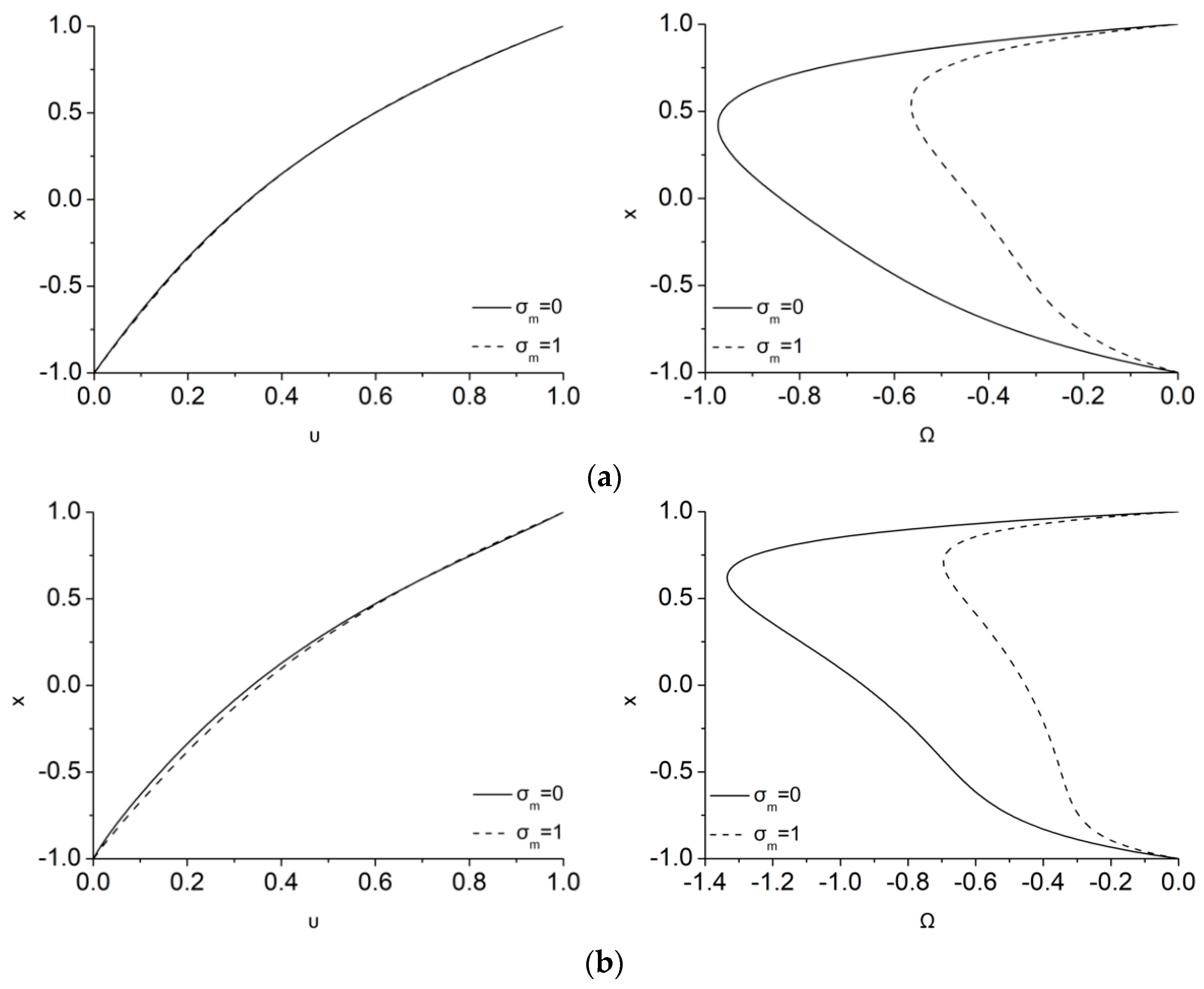
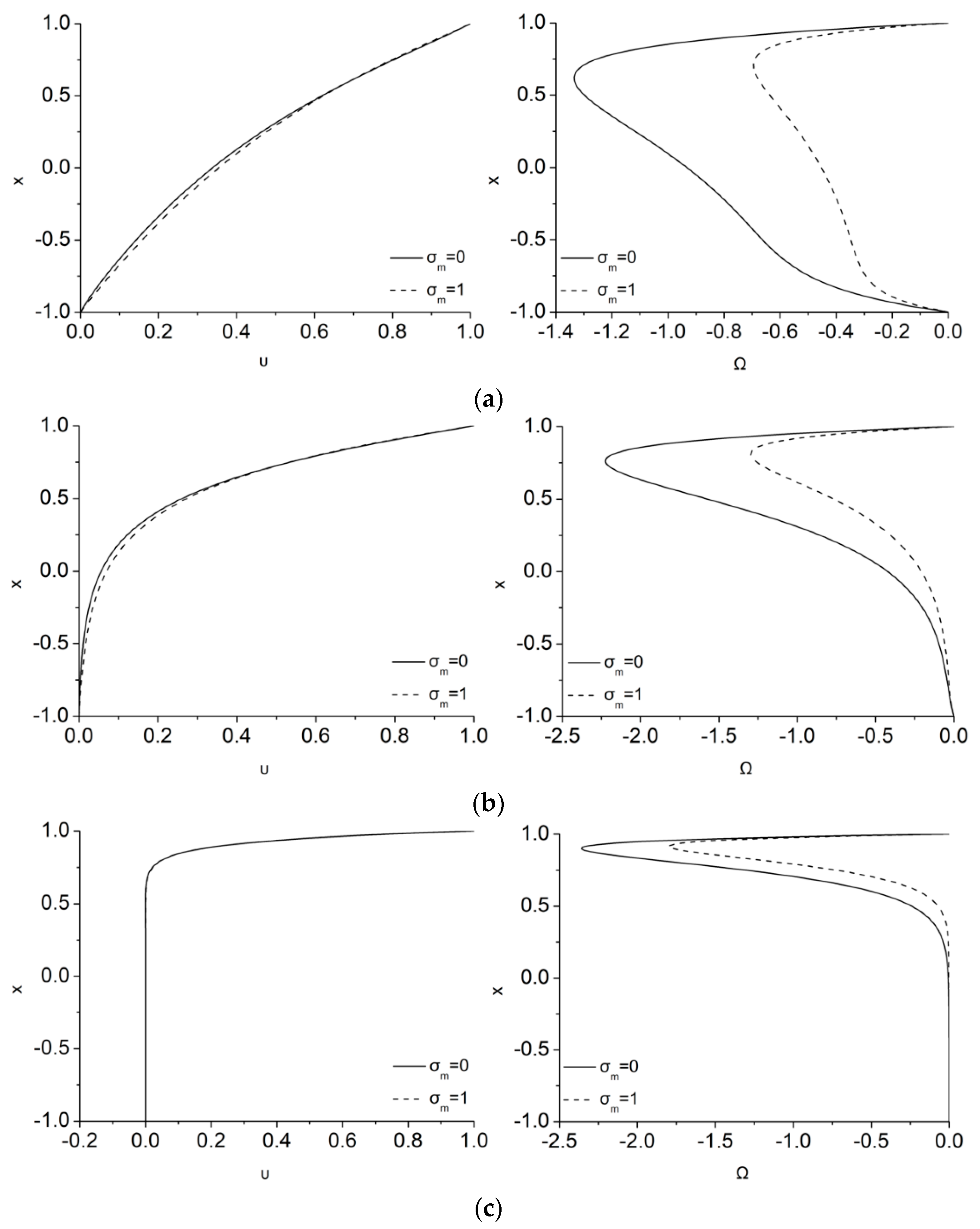
Figure 2 illustrates the influence of the magnetization parameter, ${\sigma }_m$, in the velocity and microrotation profiles for $\epsilon$ = 0.1, 0.5 and 0.9 in the case of λ = 5, Ha = 1, ζ = 0. The dimensionless velocity is kept equal to 1 at the upper plate and 0 at the lower plate, while the corresponding microrotation values at the walls are 0 as a result of setting $\delta$ = 0 at both plates. As can be gleaned from the velocity distributions of Figure 2a–c (left), in the laminar Couette flow that it is considered here, the fluid velocity profile is differentiated as compared to the usual linear hydrodynamic one owing to the effect of Lorentz forces on the conducting fluid. The magnetization parameter, ${\sigma }_m$, that it is also connected to the magnetic field can furthermore differentiate the velocity profile. An important finding is that the influence of the magnetization on the velocity profile is almost inappreciable for small values of $\epsilon$, while it gradually starts affecting the velocity as $\epsilon$ increases. This occurs because for small micropolar effect parameters the velocity profile acquires that of a Newtonian fluid. However, as $\epsilon$ increases, the microrotation increases, and the MMR term can consequently be more important.

Figure 2a–c (right) depict the effect of magnetization on the microrotation. It can be clearly seen that the consideration of a magnetization vector not parallel to the magnetic field (i.e., ${\sigma }_m$ not equal to 0) tends to decrease microrotation as $\epsilon$ increases. As a consequence, lesser dissipation is added in the flow due to the MMR term. As a result, smaller resistance to the fluid flow is anticipated, a fact that is obvious via the slight increase of the velocity that acts opposite to the flow breaking due to the Lorentz force. Thus, the usual effect of the magnetic energy to break the flow is now transferred directly through the Lorentz force and MMR terms both to linear and angular momentum, respectively, and both are breaking. Consequently, the MMR effect is in favor of the linear momentum reducing it lesser that in the usual MHD case. It should be noticed that when ${\sigma }_m=0$, i.e., in the usual MHD case, the magnetic energy affects directly only the linear momentum through the Lorentz force and only microrotation indirectly, through the velocity.

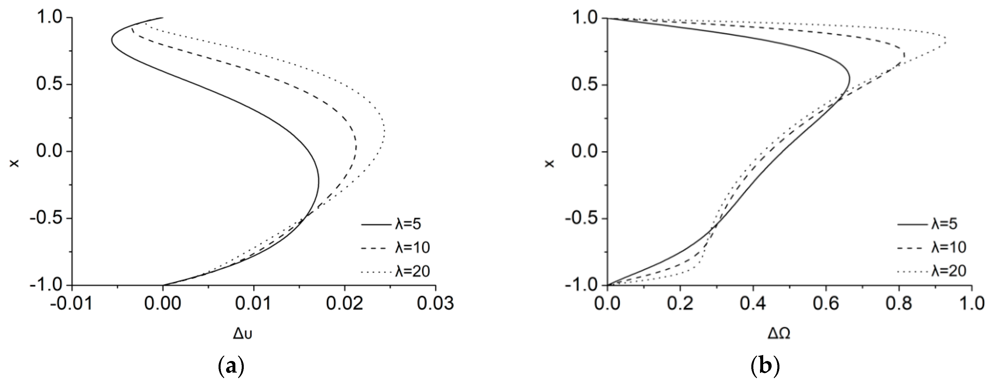
The differences in the velocity and microrotation profiles between the cases ${\sigma }_m=0$ and ${\sigma }_m=1$ are depicted in Figure 3a,b, respectively, as $\epsilon$ varies. In the laminar Couette flow that it is considered here, a difference of about 3% is measured at about $x ~ 0$ as $\epsilon \to 1$ for the velocity field. As highlighted above, the maximal value of the difference increases as $\epsilon$ increases. According to the velocity difference definition of Equation (44), its sign indicates the orientation of the ${\sigma }_m$ effect, i.e., to accelerate (for positive values) or to decelerate the flow field (for negative values). As it is shown in Figure 3a, the MMR term has the tendency to decelerate the flow field close to the upper wall and to accelerate it elsewhere in the channel. Thus, in contrast to the usual magnetic breaking that reduces analogously the flow everywhere, here, the dual magnetic action results in this more complicated energy transfer. To complete the picture, as $\epsilon \to 1$, the difference in microrotation, $\Delta \Omega$, is increased as it is shown in Figure 3b, forming its maximum of about 75% close to the upper wall, where stronger magnetic energy is transferred to microrotation through the MMR term. It should be noticed that each $\Delta \Omega$ profile is a direct measure of the corresponding MMR term’s spatial distribution.

3.2. Effect of Magnetization for Various Values of the Size Effect Parameter, $\lambda$

The size effect parameter, $\lambda$, ($\lambda =L/i$) is related to the geometry of the problem through the half height, $L$, and the microinertia, $i$, as well as the angular viscosity coefficient $\gamma$, since $\gamma =i^2\eta$. The range of $5\le \lambda <20$ is investigated in the present study and this accounts for smaller particles as the values of $\lambda$ increases, according to the relative literature [37,38]. Furthermore, since $L$ is constant, microinertia and the corresponding angular viscosity decrease as $\lambda$ increases (i.e., smaller fluid resistance). 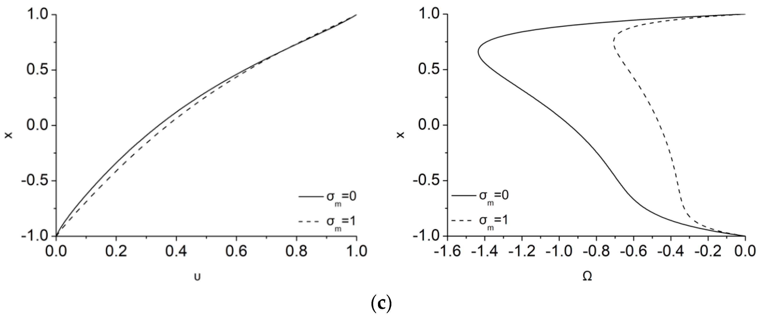In the same manner as before, Figure 4 demonstrates how the magnetization affects the velocity and microrotation for different $\lambda$ values and for ε = 0.5, Ha = 1, ζ = 0. The general formation of the flow field profile as $\lambda$ increases, is like the one discussed previously as $\epsilon$ increases, i.e., the laminar Couette flow of the study has a weak velocity increase in the middle of the channel with ${\sigma }_m$ due to the dual magnetic energy transfer. The effect of $\lambda$ is more important in microrotation distribution, since the smaller particles of the flow rotate easier as $\lambda$ increases. The dual magnetic energy breaking of the fluid’s velocities is more intense in the microrotation breaking due to the MMR term as ${\sigma }_m=1$. Thus, a part of the magnetic energy directly reduces microrotation to values even less that the half in comparison to ${\sigma }_m=0$, as seen also in the case of Figure 2 as $\epsilon$ increases, and this reduction is mostly uniform along the height of the channel.

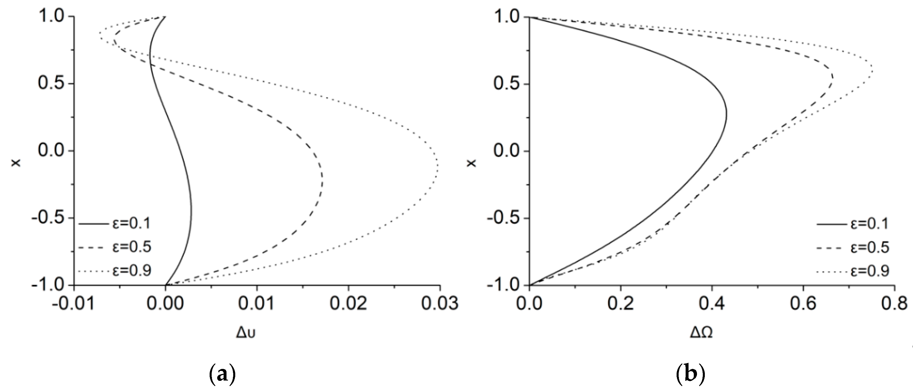
The effect of ${\sigma }_m$ as $\lambda$ varies is easier to be measured in the differences of velocity and microrotation as they are shown in Figure 5. A difference of about 2.5% is measured in velocity as $\lambda$ increases whereas, the difference in microrotation is almost up to 100%. In contrast to the $\epsilon$ increase, as $\lambda$ increases, $\Delta \upsilon$ close to the top moving wall is decreasing with tendency even to change sign, while in the rest of the channel height the difference steadily increases with $\lambda$. Moreover, as $\lambda$ increases, the MMR term make steepest the $\Delta \Omega$ distribution close to the boundary layers and reducing it in the middle of the channel. Thus, ${\sigma }_m$ is connected to the faster rotation of the smaller fluid’s particles close to the walls which dissipates faster kinetic energy inside the microrotation boundary layers and make them thicker due to higher $\lambda$.

3.3. Effect of Magnetization for Various Values of the Hartmann Number, $Ha$

The Hartmann number, $Ha$, characterizes the strength of the applied magnetic field, $H_0$, and has a range of $0\le Ha<18$ in the present analysis. In the hydrodynamic limit, no magnetic field is applied on the flow and thus $Ha$ takes the value of zero and ${\sigma }_m$ has no effect on the flow. In this case, the micropolar flow can be described by the classic Eringen’s model without the MHD and MMR considerations [2]. As $H\alpha$ number departures from zero and MHD is important, the effect of ${\sigma }_m$ in the linear and angular momentum is examined. Firstly, as expected, the increase of $H\alpha$ tends to decelerate the conducting fluid because of the increase of Lorentz forces, especially in the bulk of the fluid flow, as it is shown in Figure 6 for $Ha=1, 3$ and 18 when $\lambda =5,\epsilon =0.5,\zeta =0$. For the maximum value of $Ha$ considering here, namely for $Ha$ = 18, see Figure 6c, the fluid flow almost “freezes” as a result of Lorentz forces impact. Since in the usual Couette flow, only the velocity of the upper wall is kept constant and not the mean fluid’s mass flow, the application of the magnetic field slows down the flow and reduces its velocity magnitude everywhere in the channel. This effect, which is called Hartmann breaking, is observed in a variety of industrial applications that involve magnetic fields, such as crystal growth techniques and liquid metal blanket of nuclear fusion reactors Since the velocity of the present ideal flow is almost zero in most of the height of the channel as Hartmann number increases, the magnetization parameter has no influence on the velocity profile.

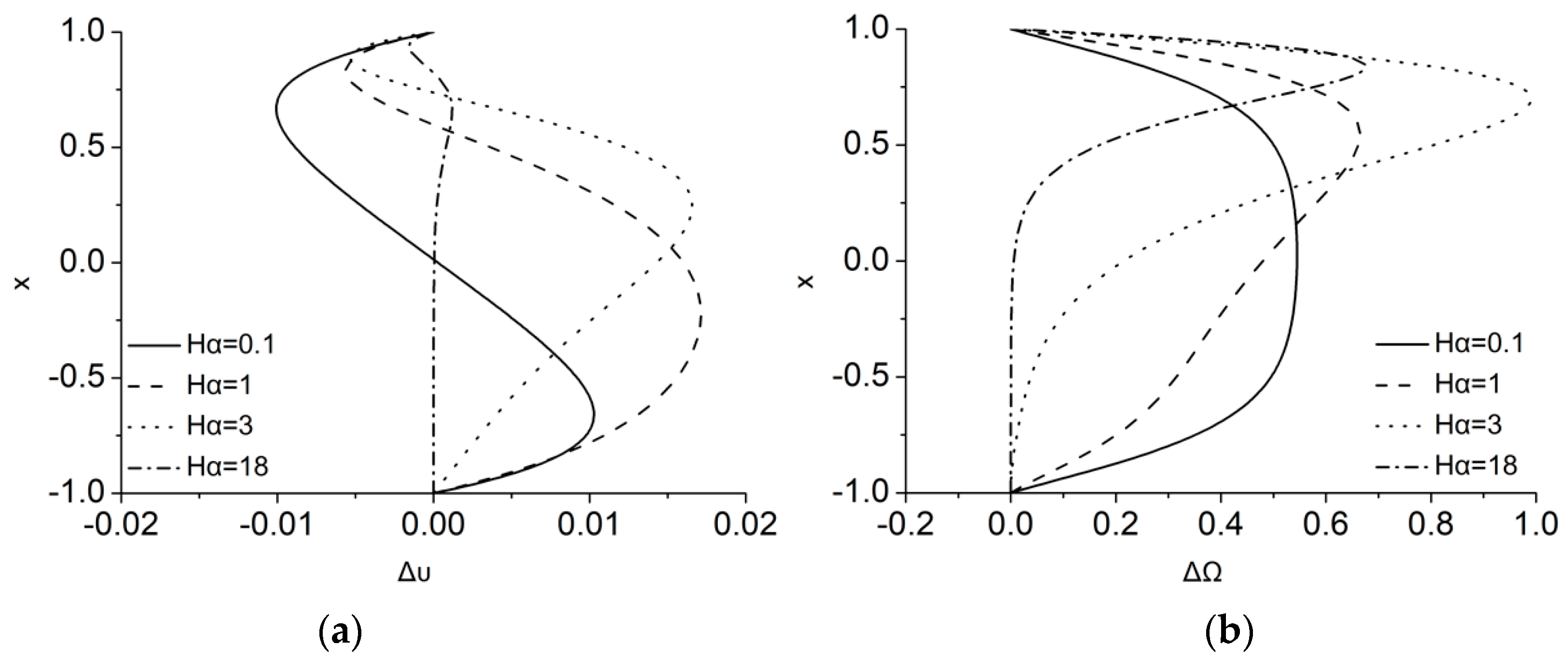
In a similar fashion as in the velocity field, as $H\alpha$ increases, microrotation is very weak and tends to zero in the bottom height of the channel, since velocity is almost zero, but maximizes in the upper part of the channel owing to the strong shearing near the moving wall. There, the MMR term is found to further reduce the rotation, in stronger rates for smaller Ha, but in slower rates, as Ha increases. This behavior is measured in the differences for velocity and microrotation that are shown in Figure 7. Overall, as the Hartmann number increases, the differences with considering or not the magnetization effect on velocity field initially increase, while as the Hartmann number further increases the fluid deceleration seems to prevail and thus the differences are minimized. The same trend is observed for the differences in microrotation due to the reduction of velocity.

Interestingly, it is observed that as $H\alpha$ increases, there is a range of values which gives for both velocity and microrotation complex number solutions. This range depends on the value of the other parameters. For example, regarding the case of $\lambda =5,\epsilon =0.5, \zeta =0$ this range is $3.6602<Ha<13.6603$ for ${\sigma }_m=0$ and $7.2474<Ha<17.2475$ for ${\sigma }_m=1$. Thus, when magnetization is considered, the minimum and the maximum values of the range, that result in the present equations, give growingly complex solutions. In

Table 1. Range of $Ha$ complex number solution for various $\lambda , \epsilon , {\sigma }_m$, and $H\alpha$.

$\mathit{\lambda }$	$\mathit{\epsilon }$	${\mathit{\sigma }}_{\mathit{m}}$	$\mathit{H}\mathit{a}$
5	0.2	0	2.8989–6.8990
5	0.2	1	4.9282–8.9283
5	0.9	0	4.0766–22.0767
5	0.9	1	9.4932–9.4933
20	0.2	0	11.5959–27.5960
20	0.2	1	19.7128–35.7129
20	0.9	0	16.3067–88.3068
20	0.9	1	37.9729–109.9730

, this range of $H\alpha$ complex number solutions for various $\lambda$ and $\epsilon$ and ${\sigma }_m=0$ or ${\sigma }_m=1$ is presented for some values of the parameters, while the electric effect parameter $\zeta$ is considered zero. It is found that, the critical $Ha$ values increase as $\lambda$ and $\epsilon$ increase. The fact that complex number solutions appear denote that possible unstable solutions are obtained, close for example to a flow bifurcation, which can be investigated via stability analysis methods that is beyond the scope of this study. However, they are mentioned here for the sake of completeness. It is also pointed out that all the analysis is done for a 2D velocity field (or, alternatively, a single component of the vorticity), and MHD is known for being the source of 3D instabilities that cannot be found in this analysis. These MHD instabilities may also be connected to the complex number solutions that we observed that usually mean the growth of temporal instabilities, i.e., a Hopf bifurcation point, that cannot also be captured by the present analysis.

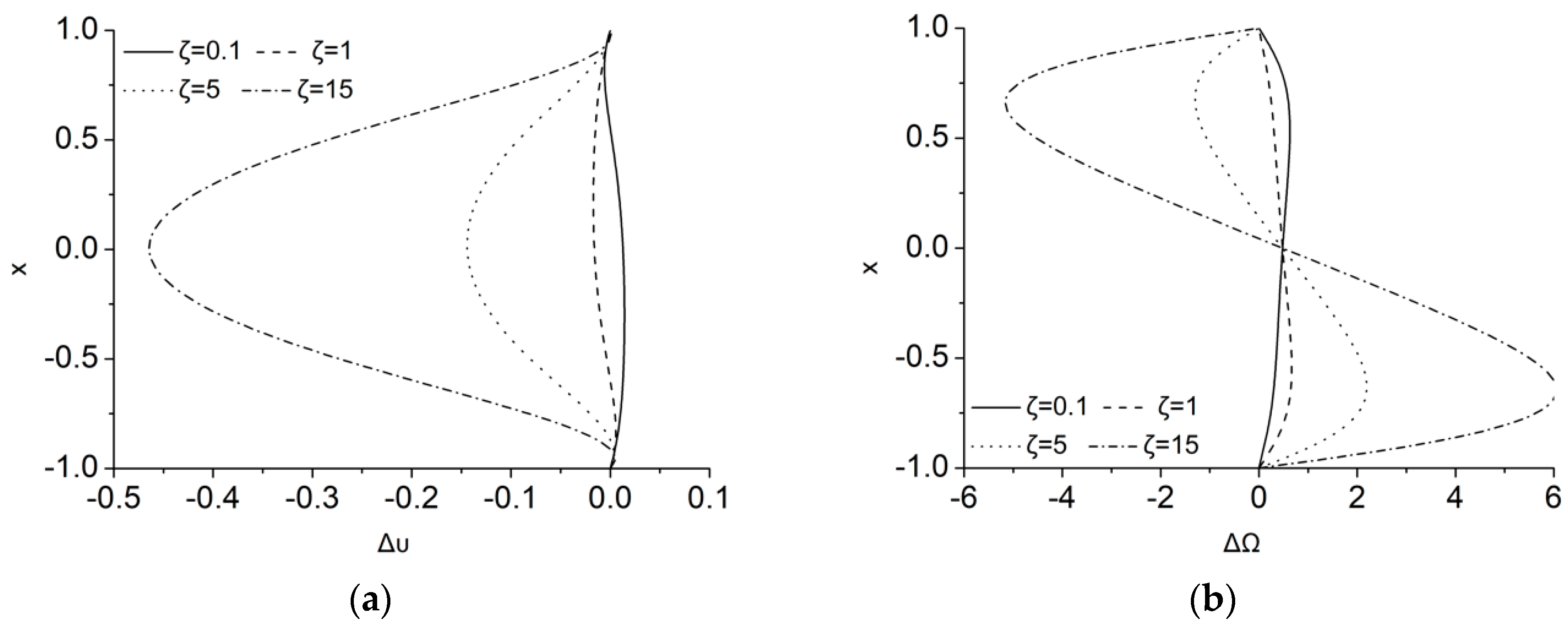
3.4. Effect of Magnetization for Various Values of the Electric Effect Parameter, ζ

The electric effect parameter, $\zeta$, characterizes the strength of the applied electric field, $E_0$, which is a flow driving force for the present configuration and it is studied in the range of $0.1\le \zeta <15$. When $\zeta$ is zero, no electric field is applied on the flow $\left(E_0=0\right)$ and the usual MHD Couette flow is recovered. In all the cases studied so far, the electric field was kept zero i.e., $\zeta =0$ to avoid modifications of the usual Couette flow characteristics. 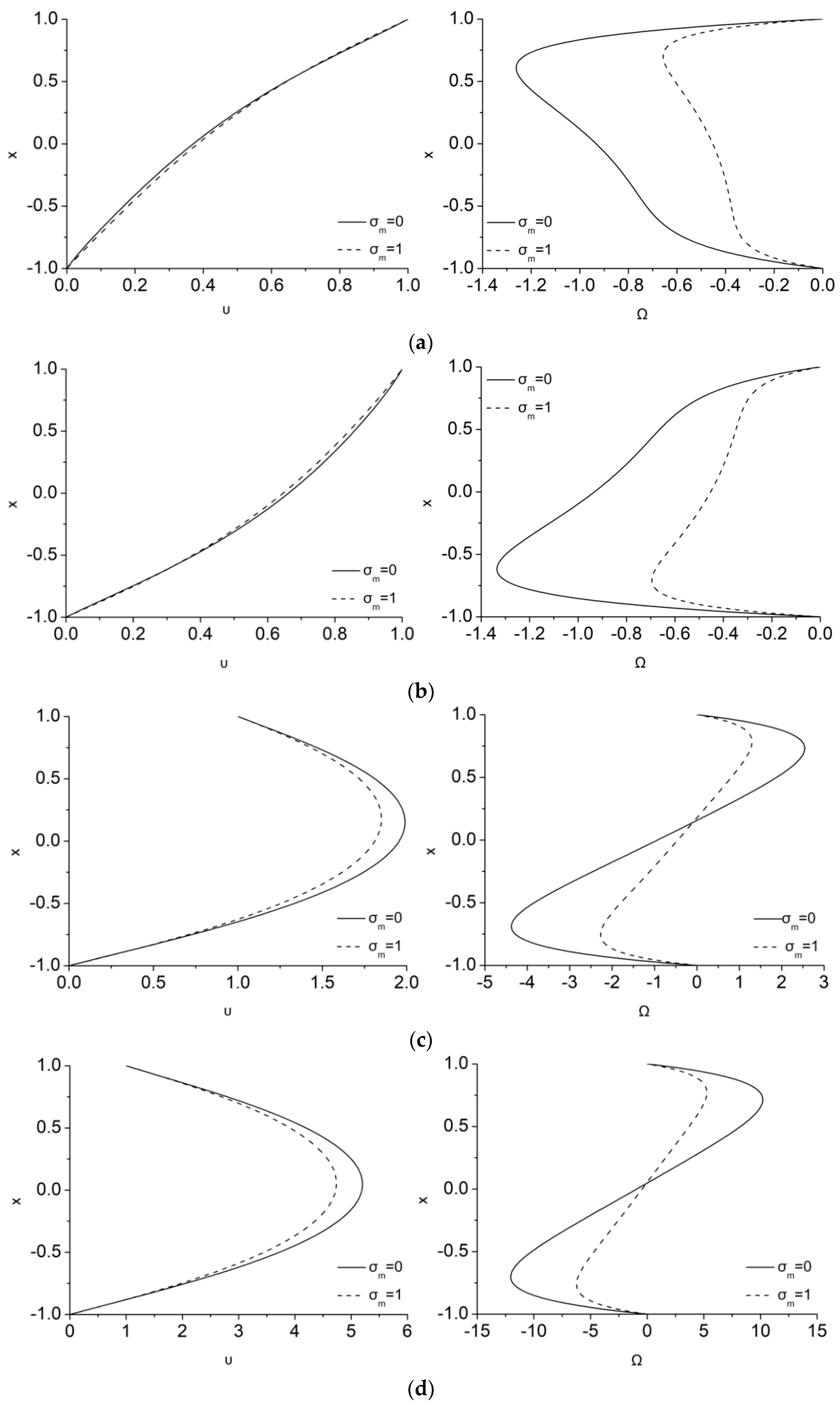Figure 8 illustrates the effect of magnetization on velocity and microrotation for different non-zero values of $\zeta$ and for ε = 0.5, λ = 5, Ha = 1. As it was expected, as $\zeta$ increases, the strong electric body force reverses the magnetic breaking, as shown in Figure 8b (left), and accelerates the fluid to obtain a parabolic, similarly to a Poiseuille flow velocity profile.

For small $\zeta$, the magnetic field decelerates the flow and the microrotation distribution is like the previous cases. However, as $\zeta$ increases the tendency of $\Omega$ is reversed. Initially, its maximum value is found near the lower wall than in the top one, Figure 8b (right), and as $\zeta$ increases, $\Omega$ in the upper part of the channel reverses its sign, shape, and even increases in magnitude everywhere in the channel as the velocity magnitude increases strongly. When magnetization is considered, both the velocity and microrotation decrease for all the cases considered here through the additional dissipation added due to the MMR term.

The MMR effect in the flow with $\zeta >0$, that is now more convective, can be measured easier through the profiles of the velocity and microrotation differences due to ${\sigma }_m$ as they were shown in Figure 9. The effect of the MMR term is now up to 45% and 600% in the velocity and microrotation fields, respectively, for the higher value of $\zeta$ considered here. Although for the $\zeta =0.1$ case the difference in the velocity and microrotation is positive, as $\zeta$ increases, this difference is getting negative for the velocity and of sinusoidal shape for the microrotation. Thus, the MMR term initially accelerates the flow due to the reduced magnetic breaking, but when momentum is stronger, acts as a dissipation term.

3.5. Effect of Magnetization on Skin Friction, $C_f$

In this subsection, the coefficient of skin friction, $C_f$, has been calculated for the upper plate of the present Couette flow and is compared against the Newtonian, the Newtonian MHD, and the micropolar Couette flows by neglecting magnetization, i.e., for ${\sigma }_m=0$. In the case of the Newtonian Couette flow, the usual mathematical relationship of $C_f{}_{Newtonian}=1/Re$ is used that can be applied for the laminar present flow, while for the MHD Couette flow the relation $C_f{}_{MHD}={\left(4/Re\right)\left(d{\upsilon }_{MHD}/dx\right)|}_{x=1}$ is utilized [39]. The solution for the MHD linear velocity was derived from Kiema et al. [40] and it is ${\upsilon }_{MHD}=\left({\mathit{e}}^{Ha\left(3+x\right)}-{\mathit{e}}^{Ha\left(1-x\right)}\right)/\left(-1+{\mathit{e}}^{4Ha}\right)$. For the micropolar Couette flow, the solution of Shiwada-Tanahashi’s model is used, which is equivalent to the solutions of Eringen’s model when the magnetization, the magnetic and the electric field are ignored $\left({\sigma }_m=0, \zeta =0,Ha=0\right)$.

The coefficient of skin friction for the five cases are given in

Table 2. $C_f$ for various $Re$ numbers.

$\mathit{R}\mathit{e}$	${\mathit{C}}_{\mathit{f}}$
	Newtonian	MHD	Micropolar	${\mathit{\sigma }}_{\mathit{m}}=0$	${\mathit{\sigma }}_{\mathit{m}}=1$	$\mathit{\delta }{\mathit{\sigma }}_{\mathit{m}}$
10	0.1000	0.4149	0.0459	0.0729	0.0802	0.73
50	0.0200	0.0830	0.0092	0.0146	0.0160	0.14
100	0.0100	0.0415	0.0046	0.0073	0.0080	0.07
200	0.0050	0.0207	0.0023	0.0036	0.0040	0.04
300	0.0033	0.0138	0.0015	0.0024	0.0027	0.03
400	0.0025	0.0104	0.0011	0.0018	0.0020	0.02
500	0.0020	0.0083	0.0009	0.0015	0.0016	0.01
600	0.0017	0.0069	0.0008	0.0012	0.0013	0.01
700	0.0014	0.0059	0.0007	0.0010	0.0011	0.01
800	0.0013	0.0052	0.0006	0.0009	0.0010	0.01
900	0.0011	0.0046	0.0005	0.0008	0.0009	0.01
1000	0.0010	0.0041	0.0004	0.0007	0.0008	0.01

for various $Re$ numbers. In case of MHD, $H\alpha =1$ is considered, while in micropolar flows $\epsilon =0.5$ and $\lambda =5$ are applied. In all cases, as expected, skin friction coefficient decreases with increasing the Reynolds number. Besides, it can be noted that $C_f$ pertaining to micropolar Couette flow is approximately half compared to that of the Newtonian flow (54% reduction). This can be noticed in various studies of skin friction coefficient such as Pal et al. [41] and Hoyt et al. [42], that showed experimentally that fluids which contain minute polymeric additives exhibit a considerable reduction in the skin friction (about 25–30%). This phenomenon can be explained very well by micropolar fluid theory. When a magnetic field is applied at the flow, the skin friction coefficient increases in all flow cases (Newtonian MHD, ${\sigma }_m=0$, ${\sigma }_m=1$). In the case of Newtonian MHD flow, there is a great increase of 315% compared to the Newtonian flow, while for micropolar flows, when the magnetic field is applied, the skin friction coefficient increases by more than 60%.

Considering micropolar flow for which magnetization is included (${\sigma }_m=1$), the skin friction coefficient is constantly higher than the case of microrotation when the magnetization is neglected (${\sigma }_m=0$). More specifically, in the last column of Table 2, the absolute difference between the two cases with ${\sigma }_m=0$ and 1 is calculated by: $\delta {\sigma }_m=\left(C_{f,{\sigma }_m=1}-C_{f,{\sigma }_m=0}\right)·100\%$. Hence, the relative difference is 0.73% for $Re=10$, while it starts decreasing until a threshold value is established, namely ${\mathsf{\delta }\mathsf{\sigma }}_{\mathrm{m}}=0.01\%$. Considering the micropolar flow in which magnetization is included $\left({\sigma }_m=1\right)$, the skin friction coefficient is slightly higher than the case of microrotation when the magnetization is neglected $\left({\sigma }_m=0\right)$, i.e., a 16% increase.

4. Conclusions

The present paper deals with the investigation of a micropolar Couette flow under uniform magnetic and electric fields. The dimensionless equations, that are similar to the Shizawa-Tanahashi model [29], are solved analytically for the velocity and microrotation. The main focus is on the effect of micromagnetorotation (MMR) that appears through the magnetization on the MHD micropolar flow. The effects of various important dimensionless parameters of the flow on velocity and microrotation are investigated along with skin friction coefficient. It is inferred that, both velocity and microrotation magnitudes, as well as their differences between solutions with and without the magnetization term, increase as λ and ε increase. Moreover, these differences for both velocity and microrotation decrease for high Hartmann number values. The difference for both velocity and microrotation also increases when the applied electric field increases. Furthermore, the skin friction coefficient of a micropolar Couette flow is smaller than the classical Newtonian Couette flow. When a magnetic field is applied, the skin friction coefficient increases for both Newtonian and micropolar Couette flow. With respect to the magnetization term in an MHD micropolar Couette flow, skin friction coefficient increases about 16% compared to an MHD micropolar Couette flow whereby the magnetization term in neglected.

Thus, reflecting on the present study, it is found that the micromagnetorotation term in the case of an MHD micropolar flow, that is connected to the magnetization of the fluid, is an important factor of the flow that is so far ignored. Thus, more intensive studies of this term should be followed to investigate deeply the MMR term effect on the micropolar fluids flow.