Abstract
Surface electromyogram (sEMG) signals are easy to record and offer valuable motion information, such as symmetric and periodic motion in human gait. Due to these characteristics, sEMG is widely used in human-computer interaction, clinical diagnosis and rehabilitation medicine, sports medicine and other fields. This paper aims to improve the estimation accuracy and real-time performance, in the case of the knee joint angle in the lower limb, using a sEMG signal, in a proposed estimation algorithm of the continuous motion, based on the principal component analysis (PCA) and the regularized extreme learning machine (RELM). First, the sEMG signals, collected during the lower limb motion, are preprocessed, while feature samples are extracted from the acquired and preconditioned sEMG signals. Next, the feature samples dimensions are reduced by the PCA, as well as the knee joint angle system is measured by the three-dimensional motion capture system, are followed by the normalization of the feature variable value. The normalized sEMG feature is used as the input layer, in the RELM model, while the joint angle is used as the output layer. After training, the RELM model estimates the knee joint angle of the lower limbs, while it uses the root mean square error (RMSE), Pearson correlation coefficient and model training time as key performance indicators (KPIs), to be further discussed. The RELM, the traditional BP neural network and the support vector machine (SVM) estimation results are compared. The conclusions prove that the RELM method, not only has ensured the validity of results, but also has greatly reduced the learning train time. The presented work is a valuable point of reference for further study of the motion estimation in lower limb.
1. Introduction
The surface electromyogram (sEMG) signal is a physiological signal, formed by the superposition of a potential difference, generated by muscle contraction or relaxation on the skin [1,2,3]. It is widely used in human-computer interaction, medical rehabilitation and other fields, because it can reflect the active strength of muscles, it is easy to acquire and offers valuable information [4,5,6,7,8]. The kinetic model, as established by the Hill model in biomechanics, can describe the motion mechanism and process, but there are still problems, such as complicated calculations and human parameters measurement of increased difficulty [9]. Combining the human body’s own bioelectrical information, such as myoelectric signals, with a machine learning method, as represented by the neural network approach, has achieved good results in muscle force and motion modeling, parameter identification and joint torque estimation [10,11,12]. The use of sEMG signals to estimate the continuous motion of human body has attracted high research interest.
For the estimation of motion, using the sEMG, the effectiveness of the method and the accuracy of the results need first to be considered. Neural networks, offering simple and direct model, are widely used in continuous motion estimation. A back propagation (BP) neural network is a kind of multi-layer feedforward neural network [13], which is derived from the adjustment rules of network weights by using a backward propagation learning algorithm. Zhang et al. used a BP neural network to estimate the joint angle of lower limbs, in normal people and patients with spinal cord injury [14]. Dai et al. estimated the ankle joint angle, through a general regression neural network (GRNN) [15]. In addition, the combination of principal component analysis (PCA), independent component analysis (ICA) and neural networks can be used to estimate the joint angle of the upper limbs [16]. Ding et al. performed continuous motion estimation, on multiple joints of upper limbs, using PCA and a high-order polynomial [17].
An important application of continuous joints motion estimation is in the motion control field of intelligent prosthetics and rehabilitation robots. Therefore, in addition to the accuracy of motion estimation, the real-time performance of the estimation algorithm is particularly important. On the one hand, during the feature extraction process of myoelectric signals, the high dimension of the data set is likely to lead to high complexity of the training model and a long training time. Therefore, it is important to find the low-dimensional data that best represents the characteristics of myoelectricity. The high correlation between the electromyographic features justifies that, some redundant sEMG features, with high correlation, be appropriately subtracted, thus improving the model training efficiency without affecting the accuracy. Practice has proved that PCA is a more practical dimension reduction method [18]. On the other hand, the learning algorithm, as represented by a BP neural network, reduces the error by gradient descent method, improving the accuracy, but falling into the local optimal solution is easy, while there is the problem of relatively long learning time. Therefore, while ensuring the validity of the method, reducing the training time of the model and avoiding falling into the local optimal solution, has become an issue of high research interest, in the field of neural networks and machine learning.
The extreme learning machine (ELM) is a new neural network algorithm, proposed by Huang, in 2004 [19]. ELM is a single hidden layer feedforward neural network. It analyzes only the output weight of the learning network, through one-step calculation. Compared to the classical BP neural network and support vector machine (SVM) [20], the ELM has significant improvement in learning speed and generalization ability, and is widely used in many fields such as face recognition [21,22,23,24]. For the complex problem of the online data collection and model training process, Liang et al. proposed online sequential extreme learning machine(OS-ELM) [25], which can effectively link the old and new training samples, while avoiding repeated training of old data. In the case of ELM, more hidden layer nodes are required, to compensate for the defects caused by random selection of hidden layer node parameters. Yang et al. proposed a two-way bidirectional extreme learning machine(B-ELM) [26], where the simulation results show that the convergence speed is high, the generalization ability is good and the structure is simple. Considering that, the traditional ELM is prone to over-fitting and affects generalization performance, some scholars have proposed a regularized extreme learning machine (RELM), which is more regular than the traditional ELM and more stable [27,28]. Abdu et al. proposed a hybrid feature extraction method with a RELM [29], which is used for accurate classification of brain tumors. The results show that this method is more efficient than the most advanced methods available. Zaineb et al. improved the ELM model via defining a recursive form [30]. Compared to the existing model, it is evident that the RELM model requires the least time in the learning phase and exhibits better performance.
Considering the requirements for effectiveness, accuracy and real-time continuous motion estimation, in terms of control, such as intelligent prosthesis and rehabilitation robot, this paper proposes a motion joint estimation method, based on sEMG information and PCA-RELM, taking the knee joint angle estimation as an example. The sEMG, collected during the movement of the lower limbs, is first dimensionally reduced by the principal component analysis method, while then the knee joint angle is estimated and verified by the RELM method.
2. Principles and Methods
2.1. sEMG Feature Extraction
The feature extraction of sEMG is usually divided into time domain analysis, frequency domain analysis, time-frequency domain analysis and nonlinear dynamics [31,32]. In the continuous motion estimation, the time domain analysis method is widely used, because of its simple calculation process. Therefore, the time domain features are used as the input features. The widely used time-domain analysis methods include mean absolute value (MAV), variance (VAR), zero crossings (ZC), logarithmic feature (Log), and waveform length (WL), etc. The equations for the EMG signal sequence x are shown as follows:
(1) Mean absolute value:
(2) Variance:
As the mean of the EMG signal is close to zero, the above equations can be simplified as:
(3) Zero crossings:
In Equation (4), .
(4) Logarithmic feature:
(5) Waveform length:
In Equations (1)–(6), the sEMG sequence is a sequence of collected samples that changes with time, where the window method is often used in actual analysis. Where, is the i-th sample point of the signal in each channel, is the average of the signals in each channel and N is the time window length for each feature extraction. In this study, in order to accurately estimate the joint angle, the sEMG of multiple muscles, related to knee joint motion, was collected, while was simultaneously pretreated.
2.2. Principal Component Analysis
Principal component analysis is a widely used mathematical dimension reduction method [18]. The main steps are as follows:
Step 1. Calculate the covariance and covariance matrix between each sample.
Let the samples be , where is the number of samples. and are any of these samples (may be the same), while the covariance is defined as:
where, represents the mean value and represents the length of the data, while their covariance matrices can be expressed as:
Step 2. Calculate the eigenvectors and eigenvalues of the covariance matrix.
Then, the eigenvalues that are solved, are sorted according to the size from large to small.
The unit eigenvectors, corresponding to the eigenvalues, are respectively:
Step 3. Calculate the principal component contribution rate and the cumulative contribution rate.
The variance contribution rate of the principal component can reflect the amount of information, described as:
The number of principal components can be determined by the cumulative contribution rate, as:
In practice, the eigenvalues, with cumulative contribution rates of 85–95%, are generally selected.
Step 4. Calculate the main components and new features after dimensionality reduction.
The selected feature vector is integrated with the original data set, while the new data set is obtained as the i-th principal component:
The first principal components are selected as the new features, after dimensionality reduction, which will be used as the input layer variables to the regularization overrun learning machine.
2.3. Regularized Extreme Learning Machine
The regularized extreme learning machine (RELM) has been widely used, due to its simple structure and fast training [19]. However, when the number of nodes in the hidden layer is too large, over-fitting is easy to occur, reducing its generalization performance. To this end, the improved RELM model [27] is adopted in this paper. The RELM structure, as illustrated in Figure 1, comprises an input layer, a hidden layer and an output layer, wherein all neurons between the layers are fully connected. each represent the number of neurons in the input layer, the hidden layer, and the output layer, respectively. and are represented as input vectors and output vectors, respectively. represents the weight between the i-th neuron of the input layer and the j-th neuron of the hidden layer, to are the thresholds of the hidden layer. is the weight between the i-th neuron of the hidden layer and the j-th neuron of the output layer.
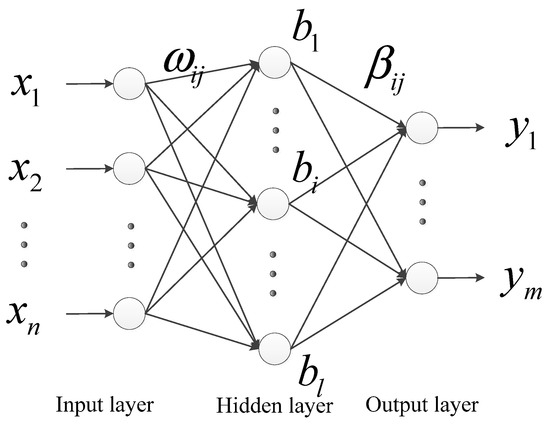
Figure 1.
Schematic diagram of regularized extreme learning machine (RELM) model.
The training sample set is (N represents the number of training samples), and represent the input and output samples of the RELM training, while the output function can be expressed as:
where, is the weight vector of the input layer and the i-th hidden layer neuron, is the weight vector of the i-th hidden layer neuron and the output layer, while is the threshold of the i-th hidden layer neuron. Abbreviating Equation (16) into a matrix form expression, leads to:
where, is represented as the hidden layer output matrix.
According to Bartlett’s theory [33], when the norm of training error and output weight are lower, the generalization is better. For this reason, the solution objective function of the network is:
where, C is the regularization coefficient, is sum of the training error, . Thus, the Lagrangian equation is,
where, is a Lagrangian operator. Deriving partial derivatives of the Equation (19):
The output weight matrix can be solved by Equation (20), while the fitted regression model of RELM is obtained, as:
Introducing in will lead to better generalization performance.
3. Experimental Data Acquisition and Processing
3.1. Experiment Process
The surface electromyography (sEMG) is used to estimate the knee joint angle. The experimental and analytical procedures are shown in Figure 2. The main steps are: acquisition of myoelectric and knee joint angle signals, pretreatment and feature extraction of myoelectric signal, PCA reduction of electromyographic feature. Dimensional, electromyographic and knee angle normalization, regularized extreme learning machine model training and testing and error analysis.

Figure 2.
Experimental flow chart.
3.2. sEMG Signal and Joint Angle Signal Acquisition
3.2.1. sEMG Signal Acquisition
In the experiments, 8 healthy men (age range: 24 ± 1.6 years old, height range: 173.4 ± 3.5 cm, body weight range: 68.0 ± 6.4 kg, no physical and mental diseases) were selected for the experiment. The external environment was kept relatively quiet, to eliminate the influence of external interference factors on the experimental results. In the subsequent data collection and analysis discussion, taking into account the individual differences between different people, when grouping experimental data, the data are grouped per participant, while the groups are sequentially recorded as G1 to G8 for eight subjects.
During the experiment, the subject sat quietly in a 0.8 m high chair with the thigh parallel to the horizontal plane and fixed. The knee joint flexed and stretched at a certain frequency, including lifting the leg and closing the leg. The whole action cycle is 2 s and each group is collected for 30 s, while each experiment is performed 5 times. At the beginning of the experiment, after the subjects were stabilized, the data was recorded again. In this paper, the sEMG signal is collected by Trigno (Delsys Inc., Natick, MA, USA), while the sampling frequency is 2000 Hz.
The muscles of the knee joint are composed of the knee extension muscles and the knee flexion-rotating muscles, which play the roles of extension and flexion rotations, respectively [34]. During the exercise of the knee joint, the knee extensors, which are mainly involved, include the medial femoral muscle, the rectus femoris muscle and the lateral femoral muscle. The knee flexion-rotating muscles include the biceps femoris, the semitendinosus and the gastrocnemius muscle. The position of the myoelectric sensor is shown in Figure 3. The sensor number and the position of the muscle are listed in Table 1. To prevent muscle fatigue from affecting the accuracy of the experiment, the participants rest for 2 min after each test.
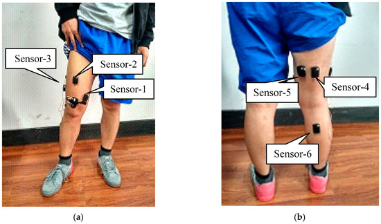
Figure 3.
Map of surface electromyogram (sEMG) sensor position. (a) Front; (b) back.

Table 1.
Sensor position.
In the experiments, raw sEMG signal from six muscles (M1 to M6) is illustrated in Figure 4. It can be seen that in the acquisition process, the collected signal is mixed with noise, which is mainly caused by sensors, environment and other factors. In order to improve the signal-to-noise ratio of the sEMG signals and reduce the effect of noise on the experimental results, a Butterworth filter is used for noise elimination [17,35], that is, firstly the acquired sEMG signal is filtered by high pass filter, then the average value is processed, and finally the low-pass filter is used.
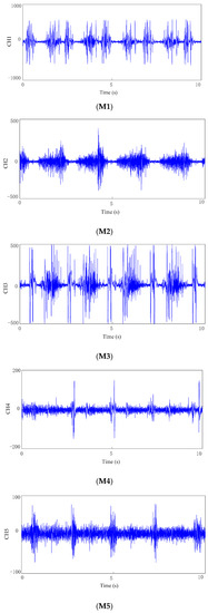
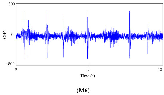
Figure 4.
EMG signals collected from different muscles.
3.2.2. Joint Angle Signal Acquisition
While collecting the sEMG, the Coda Motion 3-D Analysis System was used to record the knee joint angle signal. The Coda Motion 3-D Analysis System captures the real-time spatial location of the referring point, by capturing the infrared light marker on the sensor. Before the experiment, a 3-D coordinate system should be established, wherein the positive direction of the x-axis is directly in front of the human body, the positive direction of the y-axis is to the left side of the human body, while the positive direction of the z-axis is vertically upward. In the experiment, the sampling frequency was set to 200 Hz, while the pasting position of the marked points is as shown in Figure 5. The knee joint point is defined as point A. The knee joint is defined as point B, at the 1/3 of the hip bone. The knee joint angle is described as , during the exercise.
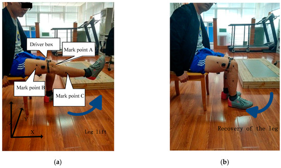
Figure 5.
Sensor location schematic diagram. (a) Leg lift; (b) leg recovery.
The three-point coordinates in three-dimensional space are: , , and , while the solution angle is . Then, , , while the following equation can be obtained:
Further available,
In this context, the obtained joint angle signal will be the output signal of the RELM model.
3.3. EMG Signal Feature Dimension Reduction
A time domain feature extraction is performed on the acquired and denoised sEMG. The time window, in the calculation, is set to 100 ms, that is, the number of sample points in the time window is 200, while the time windows do not overlap each other. In order to select the most suitable myoelectric characteristics, the first five-time domain features are extracted, namely MAV, VAR, ZC, Log, WL. Then, using the PCA method, each sEMG feature is dimensionally reduced, while the aim of accurately estimating the knee joint angle, using less data amount, is achieved.
As an example in Figure 6, the mean absolute value (MAV) of the myoelectric signal is calculated after PCA dimension reduction percentage proportion of each branch, the composition of the first four groups are 85.88%, 10.45%, 2.52%, 0.82%, which covers 99.97% of the whole data set, so the front four principal component is enough on behalf of the entire data sets, and has reached to replace the original characteristics of the corresponding requirements [18,36].
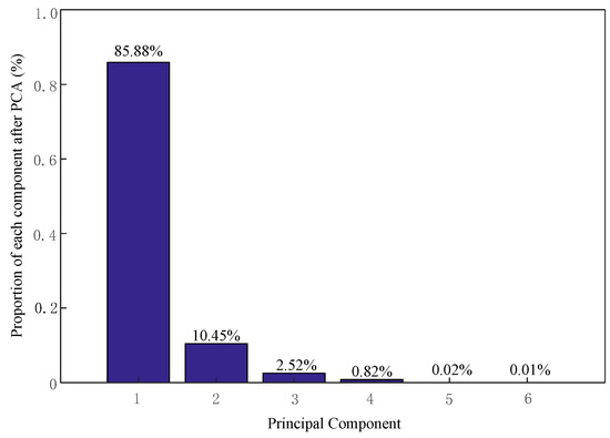
Figure 6.
The proportion of mean absolute value (MAV), after principal component analysis (PCA) reducing dimension.
In the same way, VAR, ZC, Log and WL are dimensionally reduced, while the first four groups are taken as the new eigenvalues.
3.4. Regularization Overrun Learning Machine Model Training
When the myoelectric characteristics, after PCA dimensionality reduction, as well as the knee joint angle, as measured by the three-dimensional motion capture system, are normalized, the myoelectric characteristics were used as the input layer of the RELM model, while the knee joint angle was used as the output layer. The number of hidden layers was set to 100. In order to maintain the reliability and stability of the results, this paper used the cross-validation method. According to the method presented in [37] and the characteristics of sEMG, the electromyographic feature of 30 s was divided into 3 sets with knee angle of each 10 s in experiment, among which 2 of them were selected as training data in turn, and the remaining 1 set was used as test data. The estimated angle of the knee joint was inversely normalized, compared to the real angle, while the average error was also calculated and compared with results of SVM [38] and BP neural network [14]. The data were calculated on a HP notebook computer with CPU of i5-2410 M, 2.30 GHz and memory RAM of 6 GB.
4. Results and Discussion
In order to compare the differences between different features and methods, this paper used root mean square error (RMSE) and the Pearson correlation coefficient as key performance indicators (KPIs). Wherein, the RMSE indicates the square root of the deviation, between the estimated value and the true value, while the square root of the observation No n, which can well reflect the precision of the estimation, is calculated as follows:
In addition, the Pearson correlation coefficient reflects the strength of the relationship between the two distance variables, while its value range is (−1, 1). When , they are highly correlated; when , it is a moderate correlation; when , it is a low correlation; when , it can be regarded as a nonlinear relationship.
The Pearson correlation coefficient is calculated as follows:
The angle, as measured by the three-dimensional motion capture system, is called the real angle. The angle, as estimated by the algorithm, is called the estimated angle. is the knee joint angle, as estimated by the i time algorithm, while is the mean value of the knee joint estimated angle. is the true value, measured by the three-dimensional motion capture system, at time i, while is the mean value of the true angle of the knee joint.
Next, the error analysis of different features is carried out, to compare the influence of different features on the estimation accuracy. Taking the G1 group as an example, Figure 7 shows the results of different feature prediction models in one of the experiments. The model is uniformly trained, using the same RELM. Figure 7a–e use the MAV, VAR, ZC, Log and WL, respectively, as features to train the model. The blue colored segmented lines represent the curves predicted by the RELM model, along with their respective characteristics. The solid red lines represent the curve of the true knee joint angle, during the motion. The horizontal axis is the test time and the vertical axis is the joint angle.
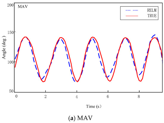
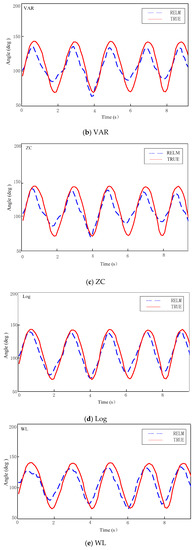
Figure 7.
Results of different feature prediction models.
Figure 7 shows that the curve, as predicted by the model of the absolute value and the logarithm, is closer to the true value, while the curve, as predicted by the variance and the zero-crossing point, is larger, while the effect of the waveform length feature is general.
The corresponding RMSE and correlation coefficient are shown in Figure 8, where it is evident that the RMSE of MAV, VAR, ZC, Log and WL are 7.113, 12.840, 13.354, 9.708 and 12.600, respectively, while the correlation coefficients are 0.9637, 0.9128, 0.8842, 0.9417 and 0.8928, respectively. Based on a comprehensive comparison of the above results, the absolute value of the mean was finally selected as the characteristic of the model.
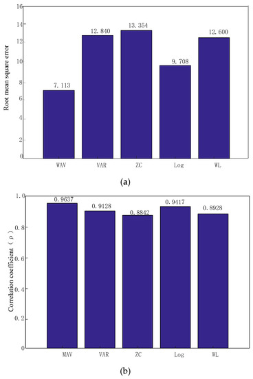
Figure 8.
Key performance indicators (KPIs). (a) Root mean square error (RMSE); (b) correlation coefficient.
Next, the analysis results of the PCA-RELM method were compared to the traditional BP neural network and SVM estimation results. Figure 9 illustrates the data of G1, under knee flexion and extension, where the horizontal axis represents the test time and the vertical axis represents the angle of the knee joint, during the exercise. The solid red line indicates the true angle value, the blue segmented line indicates the knee joint angle, estimated by the BP neural network, the brown dotted line indicates the KVM estimated knee joint angle, while the green dot line indicates the RELM estimated knee joint angle. By comparison, it was derived that the estimated values of RELM and SVM were closer to the true value, while the model appeared more stable.
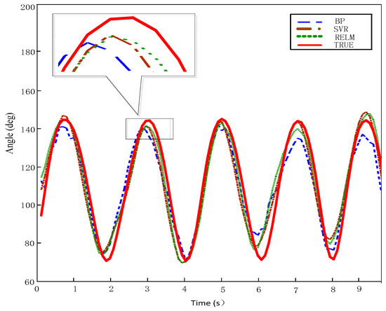
Figure 9.
Comparison of three methods to predict model results.
The error analysis of the knee joint angle estimation is shown in Table 2, as it represents the average of five experiments per person. In this paper, RMSE and correlation coefficient were used as the indicators of error analysis. This index is similar to the one described in literature [4,14]. When the root mean square value is lower and the correlation coefficient is closer to 1, it indicates that the tightness of the two sets of data is higher.

Table 2.
Knee joint angle statistics of EMG signal prediction.
Table 2 shows that the RMSE of the RELM and SVM prediction data was smaller than predicted by the BP neural network, while the correlation coefficient of the RELM and SVM prediction data was closer to one and the RELM was similar to the SVM, in accuracy. Furthermore, regarding the model training time, the RELM training time was the shortest, the SVM was the second shortest, while the BP required the longest. By comparison, it can be found that the training time of the RELM was about 1% of the BP neural network. This is so, because RELM is a single hidden layer feedforward neural network. As such, it only analyzes the output weight of the learning network, through one-step calculation, without iteration, while it has the advantage of short learning time and high generalization performance. At the same time, the traditional BP neural network requires multiple iterations, to correct the weight and threshold, because of the gradient descent method, which makes the training speed slow. In practical applications, the BP neural network is easy to fall into the local minimum point and produce suboptimal solution of learning. Therefore, RELM is more suitable for knee joint angle estimation, during exercise.
5. Conclusions
Accuracy and real-time performance are important prerequisites for continuous motion estimation. This paper proposes a PCA-RELM algorithm that uses sEMG signals to continuously estimate the knee joint angle, while it uses RMSE, correlation coefficient and model training time as indicators. Compared to traditional BP neural network and SVM, the experimental results show that the RMSE and correlation coefficient of RELM and SVM have certain similarities. The BP neural network is slightly different from the other two. Regarding training time, the RELM model requires the shortest training time, about 2–3 times faster than SVM, while two orders of magnitude higher than the requirement of the BP neural network. The presented results have certain application value for real-time identification and control of lower limb movement.
Author Contributions
Conceptualization, H.C.; methodology, F.G. and H.C.; software, H.C.; validation, H.C.; formal analysis, Y.D. and H.C.; investigation, F.G. and H.C.; resources, F.G.; data curation, H.C.; writing—original draft preparation, H.C. and Y.D.; writing—review and editing, F.G. All authors have read and agreed to the published version of the manuscript.
Funding
This research was supported by Zhejiang Provincial Natural Science Foundation of China (ZJNSF) under Grant No. LY20E050011, and National Natural Science Foundation of China (NSFC) Grant No. U1509203.
Conflicts of Interest
The authors declare no conflicts of interest.
References
- Chen, H.; Zhang, Y.; Li, G.; Fang, Y.; Liu, H. Surface electromyography feature extraction via convolutional neural network. Int. J. Mach. Learn. Cybern. 2019, 10, 1–12. [Google Scholar] [CrossRef]
- Chen, X.; Niu, X.; Wu, D.; Yu, Y.; Zhang, X. Investigation of the intra-and inter-limb muscle coordination of hands-and-knees crawling in human adults by means of muscle synergy analysis. Entropy 2017, 19, 229. [Google Scholar] [CrossRef]
- Mei, C.; Gao, F.; Li, Y. A determination method for gait event based on acceleration sensors. Sensors 2019, 19, 5499. [Google Scholar] [CrossRef] [PubMed]
- Chen, J.; Zhang, X. Surface electromyography decoding for continuous movement of human lower limb during walking. J. Xi’an Jiaotong Univ. 2016, 50, 61–67. [Google Scholar]
- Ding, Q.; Xiong, A.; Zhao, X.; Han, J. A review on researches and applications of sEMG-based motion intent recognition methods. Acta Autom. Sin. 2016, 42, 13–25. [Google Scholar]
- Artemiadis, P.K.; Kyriakopoulos, K.J. EMG-based control of a robot arm using low-dimensional embeddings. IEEE Trans. Robot. 2010, 26, 393–398. [Google Scholar] [CrossRef]
- Huang, C.; Klein, C.S.; Meng, Z.; Zhang, Y.; Li, S.; Zhou, P. Innervation zone distribution of the biceps brachii muscle examined using voluntary and electrically-evoked high-density surface EMG. J. Neuroeng. Rehabil. 2019, 16, 73. [Google Scholar] [CrossRef]
- Bingham, A.; Arjunan, S.P.; Jelfs, B.; Kumar, D.K. Normalised mutual information of high-density surface electromyography during muscle fatigue. Entropy 2017, 19, 697. [Google Scholar] [CrossRef]
- Scovil, C.Y.; Ronsky, J.L. Sensitivity of a Hill-based muscle model to perturbations in model parameters. J. Biomech. 2006, 39, 2055–2063. [Google Scholar] [CrossRef]
- Cavallaro, E.E.; Jacob, R.; Perry, J.C.; Stephen, B. Real-time myoprocessors for a neural controlled powered exoskeleton arm. IEEE Trans. Biomed. Eng. 2006, 53, 2387–2396. [Google Scholar] [CrossRef]
- Massimo Sartori, M.R.; Farina, D.; Lloyd, D.G. EMG-driven forward-dynamic estimation of muscle force and joint moment about multiple degrees of freedom in the human lower extremity. PLoS ONE 2012, 7, e52618. [Google Scholar]
- Chen, J.; Zhang, X.; Li, R. A novel design approach for lower limb rehabilitation training robot. J. Xi’an Jiaotong Univ. 2015, 49, 26–33. [Google Scholar]
- Wang, Y.; Guo, Q.; Li, W. Predictive model based on improved BP neural networks and it’s application. Comput. Meas. Control 2005, 13, 39–42. [Google Scholar]
- Zhang, F.; Li, P.; Hou, Z.G.; Lu, Z.; Chen, Y.; Li, Q.; Tan, M. sEMG-based continuous estimation of joint angles of human legs by using BP neural network. Neurocomputing 2012, 78, 139–148. [Google Scholar] [CrossRef]
- Dai, H.Q.; Zhang, J.; Shen, Z.; Zhang, L. Yanan, Application of GRNN in ankle movement prediction based on surface electromyography. Chin. J. Sci. Instrum. 2013, 34, 845–852. [Google Scholar]
- Zhang, Q.; Liu, R.; Chen, W.; Xiong, C. Simultaneous and continuous estimation of shoulder and elbow kinematics from surface EMG signals. Front. Neurosci. 2017, 11, 280. [Google Scholar] [CrossRef] [PubMed]
- Ding, Q.; Zhao, X.; Han, J. EMG-based estimation for multi-joint continuous movement of human upper limb. Robot 2014, 36, 469–476. [Google Scholar]
- Wold, S.; Esbensen, K.; Geladi, P. Principal component analysis. Chemom. Intell. Lab. Syst. 1987, 2, 37–52. [Google Scholar] [CrossRef]
- Huang, G.B.; Zhu, Q.Y.; Siew, C.K. Extreme learning machine: A new learning scheme of feedforward neural networks. Neural Netw. 2004, 2, 985–990. [Google Scholar]
- Huang, G.B.; Siew, C.K. Extreme learning machine with randomly assigned RBF kernels. Int. J. Inf. Technol. 2005, 11, 16–24. [Google Scholar]
- Mohammed, A.A.; Minhas, R.; Wu, Q.M.J.; Sid-Ahmed, M.A. Human face recognition based on multidimensional PCA and extreme learning machine. Pattern Recognit. 2011, 44, 2588–2597. [Google Scholar] [CrossRef]
- Chen, X.; Dong, Z.Y.; Meng, K.; Xu, Y.; Wong, K.P.; Ngan, H.W. Electricity price forecasting with extreme learning machine and bootstrapping. IEEE Trans. Power Syst. 2012, 27, 2055–2062. [Google Scholar] [CrossRef]
- Sun, Z.L.; Choi, T.M.; Au, K.F.; Yu, Y. Sales forecasting using extreme learning machine with applications in fashion retailing. Decis. Support Syst. 2009, 46, 411–419. [Google Scholar] [CrossRef]
- Nizar, A.H.; Dong, Z.Y.; Wang, Y. Power utility nontechnical loss analysis with extreme learning machine method. IEEE Trans. Power Syst. 2008, 23, 946–955. [Google Scholar] [CrossRef]
- Huang, G.B.; Liang, N.Y.; Rong, H.J.; Saratchandran, P.; Sundararajan, N. On-line sequential extreme learning machine. Comput. Intell. 2005, 2005, 232–237. [Google Scholar]
- Yang, Y.; Wang, Y.; Yuan, X. Bidirectional extreme learning machine for regression problem and its learning effectiveness. IEEE Trans. Neural Netw. Learn. Syst. 2012, 23, 1498–1505. [Google Scholar] [CrossRef]
- Deng, W.; Zheng, Q.; Chen, L. Regularized extreme learning machine. In Proceedings of the 2009 IEEE Symposium on Computational Intelligence and Data Mining, Nashville, TN, USA, 30 March–2 April 2009; pp. 389–395. [Google Scholar]
- Huang, G.B.; Zhou, H.; Ding, X.; Zhang, R. Extreme learning machine for regression and multiclass classification. IEEE Trans. Syst. Man Cybern. Part B 2012, 42, 513–529. [Google Scholar] [CrossRef]
- Gumaei, A.; Hassan, M.M.; Hassan, M.R.; Alelaiwi, A.; Fortino, G. A hybrid feature extraction method with regularized extreme learning machine for brain tumor classification. IEEE Access 2019, 7, 36266–36273. [Google Scholar] [CrossRef]
- Liouane, Z.; Lemlouma, T.; Roose, P.; Weis, F.; Messaoud, H. An improved extreme learning machine model for the prediction of human scenarios in smart homes. Appl. Intell. 2017, 48, 2017–2030. [Google Scholar] [CrossRef]
- Mu, Y.; Peng, C.; Zheng, X.; Zheng, E. Time-frequency analysis of surface myoelectric signals during dynamic contractions. Acta Biophys. Sin. 2004, 20, 323–328. [Google Scholar]
- Wu, Y.; Song, R. Effects of task demands on kinematics and EMG signals during tracking tasks using multiscale entropy. Entropy 2017, 19, 307. [Google Scholar] [CrossRef]
- Hansen, L.K.; Salamon, P. Neural network ensembles. IEEE Trans. Pattern Anal. Mach. Intell. 1990, 12, 993–1001. [Google Scholar] [CrossRef]
- Neumann, D.A. Kinesiology of the Kinesiology of the Musculoskeletal System: Foundations for Rehabilitation; Elsevier Health Sciences: St. Louis, MO, USA, 2013. [Google Scholar]
- Ali, A.S.; Radwan, A.G.; Soliman, A.M. Fractional order butterworth filter: Active and passive realizations. IEEE J. Emerg. Sel. Top. Circuits Syst. 2013, 3, 346–354. [Google Scholar] [CrossRef]
- Chen, H.; Gao, F.; Chen, C.; Tian, T. Estimation of ankle angle based on multi-feature fusion with random forest. In Proceedings of the 37th Chinese Control Conference (CCC 2018), Wuhan, China, 25–27 July 2018; pp. 5549–5553. [Google Scholar]
- Markatou, M.; Tian, H.; Biswas, S.; Hripcsak, G. Analysis of variance of cross-validation estimators of the generalization error. J. Mach. Learn. Res. 2005, 6, 1127–1168. [Google Scholar]
- Li, Q.L.; Song, Y.; Hou, Z.G. Estimation of lower limb periodic motions from sEMG using least squares support vector regression. Neural Process. Lett. 2015, 41, 371–388. [Google Scholar] [CrossRef]
© 2020 by the authors. Licensee MDPI, Basel, Switzerland. This article is an open access article distributed under the terms and conditions of the Creative Commons Attribution (CC BY) license (http://creativecommons.org/licenses/by/4.0/).