Lie Symmetry Analysis of Burgers Equation and the Euler Equation on a Time Scale

Abstract

As a powerful tool that can be used to solve both continuous and discrete equations, the Lie symmetry analysis of dynamical systems on a time scale is investigated. Applying the method to the Burgers equation and Euler equation, we get the symmetry of the equation and single parameter groups on a time scale. Some group invariant solutions in explicit form for the traffic flow model simulated by a Burgers equation and Euler equation with a Coriolis force on a time scale are studied.

1. Introduction

A time scale is an arbitrary nonempty closed subset of the real number set [1,2], which was initiated by Hilger to unify the continuous and discrete analysis [3]. Unification and extension are two main features of time scale calculus.

Some practical problems possess both continuous and discrete cases. Simple continuous or discrete analysis is not enough to solve problems in some compound problems. Thanks to the time scale theory, unifying results can be produced for complicated models under the frame of time scale. With the wide application and rapid development of the theory, the study of solution to dynamical equations on a time scale has raised more and more attention [4,5,6,7,8,9,10,11,12]. Peterson et al. studied the boundedness and uniqueness of solutions to dynamical equations on a time scale by defining suitable Lyapunov-type functions [6]. Hoffacker et al. investigated the stability and instability of the first-order system of dynamical equations with Lyapunov function on a time scale [7]. Amster et al. proved the existence of solutions to boundary value problem by Leray–Schauder and Brouwer degree theory on time scales [8]. Sun et al. obtained the existence of positive solutions to one-dimensional p-Laplacian boundary value problems by a fixed point theorem on a time scale [9].

The first purpose of writing this paper is to give the general Lie symmetry analysis method to dynamical equations on a time scale. It is well-known that group theory is a universal and convenient tool for analysis of partial differential equations (PDEs) and symmetry properties of PDEs have been extensively studied. As a powerful tool that can be used to solve both continuous and discrete equations, a Lie symmetry analysis method provides an effective way to solve the dynamical equations on a time scale [13,14,15,16,17,18]. To the best of our knowledge, the study of the method on this topic is still new but meaningful in solving practical problems.

The second purpose of writing this paper is to study the exact solutions to the Burgers equation and Euler equation with important physical significance on a time scale. As a nonlinear partial differential equations simulating shock wave propagation and reflection, the Burgers equation is applied widely in traffic flow, shock wave, turbulence problem, and a continuous stochastic process [19,20,21,22,23,24]. Burgers equation relates to the Navier–Stokes equation with the pressure term removed. The Euler equation is a basic hydrodynamics equation that describes the motion of inviscid fluid, which is widely applied in many fields such as fluid, astrophysics, atmospheric, and oceanic dynamics [25,26,27,28]. It relates to the Navier–Stokes equation regardless of viscosity. The study of Burger equation and Euler equation establishes foundation for the further study of Navier–Stokes equation which was considered as a famous Millennium puzzle.

In this paper, we give the Lie symmetry analysis of dynamical systems on a time scale. The main results are presented in Section 3. In Section 3.1, we investigate the Lie symmetry of dynamical equations. In Section 3.2, the method is applied to obtain the symmetry with single parameter group of the Burgers equation on a time scale, and the smooth and singular kink solutions are obtained. In Section 3.3, the method is applied to derive the symmetry with a single parameter group of the Euler equation on a time scale. The bell-shape soliton solution and solution with periodic oscillation are obtained.

2. Preliminaries

Definition 1

([2]). A time scale is an arbitrary nonempty closed subset of the real numbers.

Definition 2

([1,2]). Let $\mathbb{T}$ be a time scale.

1.

The forward jump operator $\sigma :\mathbb{T}\to \mathbb{T}$ is defined by

$$\sigma (t):=inf\{s\in \mathbb{T}:s>t\}.$$

2.

The backward jump operator $\rho :\mathbb{T}\to \mathbb{T}$ is defined by

$$\rho (t):=sup\{s\in \mathbb{T}:s<t\}.$$

3.

The graininess function $\mu :\mathbb{T}\to [0,\infty )$ is defined by

$$\mu (t):=\sigma (t)-t.$$

4.

If $\sigma (t)>t$, then t is right-scattered. If $\rho (t)<t$, then t is left-scattered. Points that are both right scattered and left-scattered are called isolated.

5.

If $t<sup\mathbb{T}$ and $\sigma (t)=t$, then t is right-dense. If $t>inf\mathbb{T}$ and $\rho (t)=t$, then t is left-dense. Points that are both right-dense and left-dense are called dense.

6.

We set $\sigma (t)=t$ if $\mathbb{T}$ has a maximum t, and $\rho (t)=t$ if $\mathbb{T}$ has a minimum t.

Consider the set ${\mathbb{T}}^{\kappa }$ that is derived from the time scale $\mathbb{T}$. If $\mathbb{T}$ has a left-scattered maximum m, then ${\mathbb{T}}^{\kappa }=\mathbb{T}-\left\{m\right\}$. Otherwise, ${\mathbb{T}}^{\kappa }=\mathbb{T}$.

Definition 3

([2]). We say a function $f:\mathbb{T}\to \mathbb{R}$ is delta differential at $t\in {\mathbb{T}}^{\kappa }$ if there is a number $f^{\Delta }(t)$ such that, for all $\epsilon >0$, there exists a neighborhood U of t (i.e., $U=(t-\delta ,t+\delta )\bigcap \mathbb{T}$ for some $\delta >0$) such that

$$\left|f(\sigma (t))-f(s)-f^{\Delta }(t)(\sigma (t)-s)\right|\le \epsilon \left|\sigma (t)-s\right|,foralls\in U.$$

We call $f^{\Delta }(t)$ the delta derivative of f at t.

In this paper, we denote ${\Delta }_{t}f:=f^{\Delta }(t)$ for ease of expression.

Proposition 1

([2]). (Leibnitz formula on a time scale) Let $S_k^{(n)}$ be the set consisting of all possible strings of length n, containing exactly k times σ and $n-k$ times Δ. If $f^{\Lambda }$ exists for all $\Lambda \in S_k^{(n)}$, then

$${(fg)}^{{\Delta }^n}=\sum _{k=0}^n(\sum _{\Lambda \in S_k^{(n)}}{f}^{\Lambda })g^{{\Delta }^k}$$

(1)

holds for all $n\in \mathbb{N}$, where $f^{\Lambda }$ denotes all possible permutations of k times σ and $n-k$ times Δ acting on f. For example, if

$$\Lambda =\{\underset{k}{\underbrace{\sigma ,\dots ,\sigma ,}}\underset{n-k}{\underbrace{\Delta ,\dots ,\Delta }}\},$$

the corresponding $f^{\Lambda }={\left(f({\sigma }^k(t))\right)}^{{\Delta }^{n-k}}$.

3. Main Results

3.1. Symmetry Analysis on a Time Scale

Theorem 1.

Considering system

$$F(t,x,u,{\Delta }_{t}u,u^{(1)},\dots ,u^{(n)})=0,t\in {\mathbb{T}}^{\kappa },x\in {\mathbb{R}}^m,u\in \mathbb{R},$$

where $x=(x_1,\dots ,x_m)$, $u^{(j)}={\partial }^{j}u/\partial x_{i_1}\partial x_{i_2}\dots \partial x_{i_j}=u_{i_1{i}_2\dots i_j}$, $i_j=1,2,\dots ,m,$ for $j=1,2,\dots ,n$ corresponding to all jth-order partial derivatives of u with respect to $x$. Let $\underset{-}{V}=\tau (t,x,u){\Delta }_t+{\displaystyle \sum _{i=1}^m}{\xi }_i(t,x,u)\frac{\partial }{\partial x_i}+\varphi (t,x,u)\frac{\partial }{\partial u}$ be a vector on open set M defined on ${\mathbb{T}}^{\kappa }\times X\times \mathit{U}$, then the nth-order prolongation of $\underset{-}{V}$ is

$${\mathrm{Pr}}^{(n)}\underset{-}{V}=\underset{-}{V}+\sum _J{\varphi }^J(t,x,u^{(n)})\frac{\partial }{\partial ({\Delta }_{J}u)},$$

where

$${\varphi }^J(t,x,u^{(n)})=T_J(\varphi -(\tau {\Delta }_{t}u+\sum _{i=1}^m{\xi }_i\frac{\partial u}{\partial x_i}))+\tau ({\sigma }^k(t),x,u){\Delta }_J{\Delta }_{t}u+\sum _{i=1}^m{\xi }_i({\sigma }^k(t),x,u){\Delta }_J\frac{\partial u}{\partial x_i},$$

$J=\left(j_1,\dots ,j_i\right),1\le i\le n,j_i\in \{t,x\}$, ${\sigma }^k(t)={\underbrace{\sigma \circ \sigma \dots .\circ \sigma }}_k(t)$, the index k in ${\sigma }^k(t)$ denotes the number that satisfies $j_i=t$ for $i=1,\dots ,n.$

As $j_i=t$,

$$T_t(\varphi (t,x,u^{(n)})=\frac{\Delta \varphi }{\Delta t}+\frac{\Delta u}{\Delta t}\frac{\partial \varphi (t,x,u^n(\overline{t},x)}{\partial u}+\sum _J\frac{\Delta u_J}{\Delta t}\frac{\partial \varphi (t,x,u^{(n)}(\overline{t},x))}{\partial u_J}(\overline{t}\in (t,\sigma (t))),$$

where $\frac{\Delta \varphi }{\Delta t}={\Delta }_t\varphi$.

As $j_i=x_k\in \left\{x\right\}$, $x=\sigma (x)$, ${\Delta }_{j_i}\varphi =\frac{\partial \varphi }{\partial x_k}$,

$$T_{j_i}(\varphi (t,x,u^{(n)}(t,x))=D_{x_k}(\varphi (t,x,u^{(n)}(t,x))=\frac{\partial \varphi }{\partial x_k}+\frac{\partial u}{\partial x_k}\frac{\partial \varphi (t,x,u^n(t,x)}{\partial u}+\sum _J\frac{\partial u_J}{\partial x_k}\frac{\partial \varphi (t,x,u^{(n)}(t,x))}{\partial u_J},$$

where $u_J={\Delta }_{J}u\in \{{\Delta }_{t}u,u^{(1)},u^{(2)},\dots ,u^{(n)}\}$.

Proof. 

We prove Theorem 1 by induction on $n\in {\mathbb{N}}^{\ast }.$ Let us first initialize the proof for $n=1.$ As $n=1$, $g_{\epsilon }=\exp (\epsilon \underset{-}{V})$ is a one-parameter semigroup corresponding to $\underset{-}{V}$,

$$(\tilde{t},\tilde{\mathbf{x}},\tilde{u})=g_{\epsilon }(t,\mathbf{x},u)=({\Psi }_{\epsilon }(t,\mathbf{x},u),{\Phi }_{\epsilon }(t,\mathbf{x},u)),\mathrm{where}(\tilde{t},\tilde{\mathbf{x}})={\Psi }_{\epsilon }(t,\mathbf{x},u).$$

Let $(t,\mathbf{x},u^{(1)})\in M^{(1)}$, $u=f(t,\mathbf{x})$ satisfy

$$u^{(1)}={\mathrm{Pr}}^{(1)}f(t,\mathbf{x}),$$

i.e., $u=f(t,\mathbf{x})$, ${\Delta }_{t}u={\Delta }_{t}f(t,\mathbf{x})$, ${\partial }_{x}u={\partial }_{x}f(t,\mathbf{x})$. While $\epsilon$ is sufficiently small, $f\to \tilde{f}$, i.e.,

$$\tilde{u}={\tilde{f}}_{\epsilon }(\tilde{t},\tilde{\mathbf{x}})=(g_{\epsilon }\circ f)(\tilde{t},\tilde{\mathbf{x}})={\Phi }_{\epsilon }(t,\mathbf{x},f)={\Phi }_{\epsilon }\circ (1\times f)(t,\mathbf{x}),$$

where 1 means identity transformation. By

$$(\tilde{t},\tilde{\mathbf{x}})={\Psi }_{\epsilon }(t,\mathbf{x},f)={\Psi }_{\epsilon }\circ (1\times f)(t,\mathbf{x}),$$

we have

$$(t,\mathbf{x})={({\Psi }_{\epsilon }\circ (1\times f))}^{-1}(\tilde{t},\tilde{\mathbf{x}}),$$

then

$$\tilde{u}={\tilde{f}}_{\epsilon }(\tilde{t},\tilde{\mathbf{x}})=({\Phi }_{\epsilon }\circ (1\times f))\circ {({\Psi }_{\epsilon }\circ (1\times f))}^{-1}(\tilde{t},\tilde{\mathbf{x}}).$$

Let $H\tilde{f}=({\Delta }_{\tilde{t}}\tilde{f},{\partial }_{\tilde{\mathbf{x}}}\tilde{f})$, then

$$H{\tilde{f}}_{\epsilon }(\tilde{t},\tilde{\mathbf{x}})=\left(H({\Phi }_{\epsilon }\circ (1\times f)(t,\mathbf{x}))\right){\left(H({\Psi }_{\epsilon }\circ (1\times f)(t,\mathbf{x}))\right)}^{-1},$$

and

$${\Psi }_0(t,\mathbf{x},f(t,\mathbf{x}))=(t,\mathbf{x}),{\Phi }_0(t,\mathbf{x},f(t,\mathbf{x}))=f(t,\mathbf{x}),$$

$$H\left({\Psi }_0(1\times f)\right)(t,\mathbf{x})=I,H\left({\Phi }_0(1\times f)\right)(t,\mathbf{x})=Hf(t,\mathbf{x}),$$

where I is an identity matrix. Then,

$$\begin{array}{cc}& {\left.\frac{d}{d\epsilon }H{\tilde{f}}_{\epsilon }(\tilde{t},\tilde{\mathbf{x}})\right|}_{\epsilon =0}\hfill \\ \hfill =& {\left.\frac{d}{d\epsilon }\left(H{\Phi }_{\epsilon }\circ (1\times f)\right)(t,\mathbf{x})\right|}_{\epsilon =0}-{\left.Hf(t,\mathbf{x})\frac{d}{d\epsilon }H\left({\Psi }_{\epsilon }\circ (1\times f)\right)(t,\mathbf{x})\right|}_{\epsilon =0}\hfill \\ \hfill =& H\left(\varphi \circ (1\times f)\right)(t,\mathbf{x})-Hf(t,\mathbf{x})H\left((\tau ,\xi )\circ (1\times f)\right)(t,\mathbf{x}),\hfill \end{array}$$

where

$$Hf(t,\mathbf{x})=\left({\Delta }_{t}f,{\partial }_{x_1}f,\dots ,{\partial }_{x_m}f\right),$$

$$H((\tau ,\xi ){}^{\circ }(1\times f))(t,\mathbf{x})=\left(\begin{array}{cc}{T}_t(\tau (t,\mathbf{x},f(t,\mathbf{x})))& D_{\mathbf{x}}(\tau (t,\mathbf{x},f(t,\mathbf{x})))\\ T_t({\xi }_1(t,\mathbf{x},f(t,\mathbf{x})))& D_{\mathbf{x}}({\xi }_1(t,\mathbf{x},f(t,\mathbf{x})))\\ ⋮& ⋮\\ T_t({\xi }_m(t,\mathbf{x},f(t,\mathbf{x})))& D_{\mathbf{x}}({\xi }_m(t,\mathbf{x},f(t,\mathbf{x})))\end{array}\right).$$

Then,

$$Hf(t,\mathbf{x})H((\tau ,\xi )\circ (1\times f))(t,\mathbf{x})={\left(\begin{array}{c}{\Delta }_{t}f·T_t\left(\tau (t,\mathbf{x},f(t,\mathbf{x}))\right)+{\displaystyle \sum _{i=1}^m}{\partial }_{x_i}f·T_t\left({\xi }_i(t,\mathbf{x},f(t,\mathbf{x}))\right)\\ {\Delta }_{t}f·D_{\mathbf{x}}\left(\tau (t,\mathbf{x},f(t,\mathbf{x}))\right)+{\displaystyle \sum _{i=1}^m}{\partial }_{x_i}f·D_{\mathbf{x}}\left({\xi }_i(t,\mathbf{x},f(t,\mathbf{x}))\right)\end{array}\right)}^T.$$

The coefficient of ${\Delta }_{t}u$ in ${\mathrm{Pr}}^{(1)}\underset{-}{V}$ corresponds to the first component of ${\left.\frac{d}{d\epsilon }H{\tilde{f}}_{\epsilon }(\tilde{t},\tilde{\mathbf{x}})\right|}_{\epsilon =0}$. The coefficient of ${\partial }_{\mathbf{x}}u$ in ${\mathrm{Pr}}^{(1)}\underset{-}{V}$ corresponds to the second component of ${\left.\frac{d}{d\epsilon }H{\tilde{f}}_{\epsilon }(\tilde{t},\tilde{\mathbf{x}})\right|}_{\epsilon =0}$. Thus,

$$\begin{array}{cc}& {\varphi }^t(t,\mathbf{x},{\mathrm{Pr}}^{(1)}f(t,\mathbf{x}))\hfill \\ \hfill =& T_t(\varphi (t,\mathbf{x},f(t,\mathbf{x})))-\left[{\Delta }_{t}f·T_t\left(\tau (t,\mathbf{x},f(t,\mathbf{x}))\right)+\sum _{i=1}^m{\partial }_{x_i}f·T_t\left({\xi }_i(t,\mathbf{x},f(t,\mathbf{x}))\right)\right],\hfill \end{array}$$

$$\begin{array}{cc}& {\varphi }^{x_k}(t,\mathbf{x},{\mathrm{Pr}}^{(1)}f(t,\mathbf{x}))\hfill \\ \hfill =& D_{x_k}(\varphi (t,\mathbf{x},f(t,\mathbf{x})))-\left[{\Delta }_{t}f·D_{x_k}\left(\tau (t,\mathbf{x},f(t,\mathbf{x}))\right)+\sum _{i=1}^m{\partial }_{x_i}f·D_{x_k}\left({\xi }_i(t,\mathbf{x},f(t,\mathbf{x}))\right)\right],\hfill \end{array}$$

where $T_t(\varphi (t,\mathbf{x},u(t,\mathbf{x}))=\frac{\Delta \varphi }{\Delta t}+\frac{\Delta u}{\Delta t}\frac{\partial \varphi (t,x,u(\overline{t},x)}{\partial u}(\overline{t}\in (t,\sigma (t))),D_{x_k}=\frac{\partial }{\partial x_k}+\frac{\partial u}{\partial x_k}\frac{\partial }{\partial u}.$

Then, by Proposition (1),

$$\begin{array}{cc}& {\varphi }^t(t,\mathbf{x},u^{(1)})\hfill \\ \hfill =& T_t(\varphi (t,\mathbf{x},u))-({\Delta }_{t}u·T_t(\tau (t,\mathbf{x},u))+\sum _{i=1}^m{\partial }_{x_i}u·T_t({\xi }_i(t,\mathbf{x},u)))\hfill \\ \hfill =& T_t(\varphi -(\tau (t,\mathbf{x},u){\Delta }_{t}u+\sum _{i=1}^m{\xi }_i(t,\mathbf{x},u){\partial }_{x_i}u))+\tau (\sigma (t),\mathbf{x},u){\Delta }_t^{2}u+\sum _{i=1}^m{\xi }_i(\sigma (t),\mathbf{x},u){\Delta }_t{\partial }_{x_i}u\hfill \end{array}$$

and

$$\begin{array}{cc}\hfill {\varphi }^{x_k}(t,\mathbf{x},u^{(1)})=& D_{x_k}(\varphi -(\tau (t,\mathbf{x},u){\Delta }_{t}u+\sum _{i=1}^m{\xi }_i(t,\mathbf{x},u){\partial }_{x_i}u))\hfill \\ \hfill +& \tau (t,\mathbf{x},u){\partial }_{x_k}{\Delta }_t^{}u+\sum _{i=1}^m{\xi }_i(t,\mathbf{x},u){\partial }_{x_k}{\partial }_{x_i}u,\hfill \end{array}$$

which means that the theorem holds for $n=1$.

Assuming the conclusion holds for $n-1$, we prove that it also holds for n. As $M^{(n)}$ can be considered as the subspace of 1-order prolongation ${(M^{(n-1)})}^{(1)}$ of $M^{(n-1)}$, then ${\mathrm{Pr}}^{(n)}\underset{-}{V}$ can be obtained by the 1-order prolongation of ${\mathrm{Pr}}^{(n-1)}\underset{-}{V}$. Thus, the coefficient of ${\mathrm{Pr}}^{(n)}V$ is

$${\varphi }^{\widehat{J}}(t,\mathbf{x},u^{(n-1)})=T_{\widehat{J}}(\varphi -(\tau {\Delta }_{t}u+\sum _{i=1}^m{\xi }_i{\partial }_{x_i}u))+\tau ({\sigma }^{\widehat{k}}(t),\mathbf{x},u){\Delta }_{\widehat{J}}{\Delta }_{t}u+\sum _{i=1}^m{\xi }_i({\sigma }^{\widehat{k}}(t),\mathbf{x},u){\Delta }_{\widehat{J}}{\partial }_{x_i}u,$$

where $\widehat{J}=(j_1,\dots ,j_i)$, $1\le i\le n-1$, the index $\widehat{k}\mathrm{in}{\sigma }^{\widehat{k}}(t)\mathrm{denotes}\mathrm{the}\mathrm{number}\mathrm{that}\mathrm{satisfies}{j}_i=t\mathrm{for}i=1,\dots ,n-1.$ Similar to the 1-order prolongation of ${\mathrm{Pr}}^{(n-1)}\underset{-}{V}$, the coefficient of

$$\begin{array}{cc}\hfill {\varphi }^{\widehat{J},j_n}& =T_{j_n}(T_{\widehat{J}}(\varphi -(\tau {\Delta }_{t}u+\sum _{i=1}^m{\xi }_i{\partial }_{x_i}u)))\hfill \\ & +\tau ({\sigma }^k(t),\mathbf{x},u){\Delta }_{\widehat{J}}{\Delta }_{j_n}{\Delta }_{t}u+\sum _{i=1}^m{\xi }_i({\sigma }^k(t),\mathbf{x},u){\Delta }_{\widehat{J}}{\Delta }_{j_n}{\partial }_{x_i}u\hfill \\ & =T_J(\varphi -(\tau {\Delta }_{t}u+\sum _{i=1}^m{\xi }_i{\partial }_{x_i}u))+\tau ({\sigma }^k(t),\mathbf{x},u){\Delta }_J{\Delta }_{t}u+\sum _{i=1}^m{\xi }_i({\sigma }^k(t),\mathbf{x},u){\Delta }_J{\partial }_{x_i}u,\hfill \end{array}$$

$J=\left(j_1,\dots ,j_i\right)$, $1\le i\le n-1$, $j_i\in \{t,\mathbf{x}\}$, the index k in ${\sigma }^k(t)$ denotes the number that satisfies $j_i=t$ for $i=1,\dots ,n.$  □

3.2. Lie Symmetry Analysis of the Burgers Equation on a Time Scale

For a (1+1)-dimensional Burgers equation with constant coefficients on a time scale,

$${\Delta }_{t}v-2Av{v}_x-B{v}_{xx}=0,t\in {\mathbb{T}}^{\kappa },x\in \mathbb{R}.$$

(2)

Let $v=u_x$; we obtain the potential form of the Burgers equation

$${\Delta }_{t}u-A{u}_x^2-B{u}_{xx}=C,t\in {\mathbb{T}}^{\kappa },x\in \mathbb{R}.$$

(3)

The Lie algebra of Equation (3) is spanned by the following vector field

$$V=\tau (t,x,u){\Delta }_t^{}+\xi (t,x,u){\partial }_x+\varphi (t,x,u)\frac{\partial }{\partial u}.$$

(4)

The infinitesimal invariance criterion of Equation (3) can be written as

$${\left.{\mathrm{Pr}}^{(2)}V(E)\right|}_{E=0}=0,$$

where $E={\Delta }_{t}u-A{u}_x^2-B{u}_{xx}-C$. The operator ${\mathrm{Pr}}^{(2)}V$ has the following form:

$${\mathrm{Pr}}^{(2)}V=V+{\varphi }^t\frac{\partial }{\partial ({\Delta }_{t}u)}+{\varphi }^x\frac{\partial }{\partial u_x}+{\varphi }^{xx}\frac{\partial }{\partial u_{xx}}+{\varphi }^{tx}\frac{\partial }{\partial {({\Delta }_{t}u)}_x}+{\varphi }^{tt}\frac{\Delta }{{\Delta }_t^{2}u}.$$

The determining equation is

$${\varphi }^t-2A{u}_x{\varphi }^x-B{\varphi }^{xx}=0,$$

(5)

with

$$\begin{array}{cc}\hfill {\varphi }^t& =T_t(\varphi -\tau {\Delta }_{t}u-\xi u_x)+\tau (\sigma (t),\mathbf{x},u){\Delta }_t^{2}u+\xi (\sigma (t),\mathbf{x},u){\Delta }_t{u}_x\hfill \\ & ={\Delta }_t\varphi +(\frac{\partial \varphi (t,x,u(\overline{t},x))}{\partial u}-{\Delta }_t\tau ){\Delta }_{t}u-{\tau }_u{\Delta }_t^{2}u-{\Delta }_t\xi u_x-{\xi }_u{u}_x{\Delta }_{t}u,\hfill \\ \hfill {\varphi }^x& =D_x(\varphi -\tau {\Delta }_{t}u-\xi u_x)+\tau (t,x,u){\Delta }_t^{}{u}_x+\xi (t,x,u)u_{xx}\hfill \\ & ={\varphi }_x+({\varphi }_u-{\xi }_x)u_x-{\tau }_x{\Delta }_t^{}u-{\xi }_u{u}_x^2-{\tau }_u{u}_x{\Delta }_{t}u,\hfill \\ \hfill {\varphi }^{xx}& =D_x^2(\varphi -\tau {\Delta }_{t}u-\xi u_x)+\tau u_{xxt}+\xi u_{xxx}\hfill \\ & ={\varphi }_{xx}+(2{\varphi }_{xu}-{\xi }_{xx})u_x-{\tau }_{xx}{\Delta }_{t}u+({\varphi }_{uu}-2{\xi }_{xu})u_x^2\hfill \\ & -2{\tau }_{xu}{u}_x{\Delta }_{t}u-{\xi }_{uu}{u}_x^3-{\tau }_{uu}{u}_x^2{\Delta }_{t}u+({\varphi }_u-2{\xi }_x)u_{xx}\hfill \\ & -2{\tau }_x{\Delta }_t(u_x)-3{\xi }_u{u}_{xx}{u}_x-{\tau }_u{u}_{xx}{\Delta }_{t}u-2{\tau }_u({\Delta }_t{u}_x)u_x.\hfill \end{array}$$

Thus, the determining Equation (5) is converted to

$$\begin{array}{cc}\hfill & {\varphi }^t-2A{u}_x{\varphi }^x-B{\varphi }^{xx}\hfill \\ \hfill =& {\Delta }_t\varphi +(\frac{\partial \varphi (t,x,u(\overline{t},x))}{\partial u}-{\Delta }_t\tau ){\Delta }_{t}u-{\tau }_u{\Delta }_t^{2}u-{\Delta }_t\xi u_x-{\xi }_u{u}_x{\Delta }_{t}u\hfill \\ \hfill -& 2A{u}_x({\varphi }_x+({\varphi }_u-{\xi }_x)u_x-{\tau }_x{\Delta }_t^{}u-{\xi }_u{u}_x^2-{\tau }_u{u}_x{\Delta }_{t}u)\hfill \\ \hfill -& B({\varphi }_{xx}+(2{\varphi }_{xu}-{\xi }_{xx})u_x-{\tau }_{xx}{\Delta }_{t}u+({\varphi }_{uu}-2{\xi }_{xu})u_x^2\hfill \\ \hfill -& 2{\tau }_{xu}{u}_x{\Delta }_{t}u-{\xi }_{uu}{u}_x^3-{\tau }_{uu}{u}_x^2{\Delta }_{t}u+({\varphi }_u-2{\xi }_x)u_{xx}\hfill \\ \hfill -& 2{\tau }_x{\Delta }_t(u_x)-3{\xi }_u{u}_{xx}{u}_x-{\tau }_u{u}_{xx}{\Delta }_{t}u-2{\tau }_u({\Delta }_t{u}_x)u_x)\hfill \end{array}$$

(6)

from which the Lie point symmetry group can be ascertained. Firstly, from the fact that the coefficients of ${\Delta }_t{u}_x,({\Delta }_t{u}_x)u_x,u_{xx}{u}_x$ in Equation (6) being 0, we have

$${\tau }_x=0,{\tau }_u=0,{\xi }_u=0.$$

(7)

Furthermore, substituting Equation (7) into Equation (6), we get

$$\begin{array}{cc}\hfill & {\varphi }^t-2A{u}_x{\varphi }^x-B{\varphi }^{xx}\hfill \\ \hfill =& {\Delta }_t\varphi +(\frac{\partial \varphi (t,x,u(\overline{t},x))}{\partial u}-{\Delta }_t\tau )(A{u}_x^2+B{u}_{xx}+C)-{\Delta }_t\xi u_x-2A{u}_x({\varphi }_x+({\varphi }_u-{\xi }_x)u_x)\hfill \\ \hfill -& B({\varphi }_{xx}+(2{\varphi }_{xu}-{\xi }_{xx})u_x+{\varphi }_{uu}{u}_x^2+({\varphi }_u-2{\xi }_x)u_{xx}).\hfill \end{array}$$

(8)

The coefficients of $u_{xx},u_x^2,u_x,1$ in Equation (8) should be 0,

$$\begin{array}{cc}\hfill u_{xx}& :B\left(\frac{\partial \varphi (t,x,u(\overline{t},x))}{\partial u}-{\Delta }_t\tau -{\varphi }_u+2{\xi }_x\right)=0\hfill \\ \hfill u_x^2& :B{\varphi }_{uu}+A\frac{\partial \varphi (t,x,u(\overline{t},x))}{\partial u}+A{\Delta }_t\tau -2A{\xi }_x=0\hfill \\ \hfill u_x& :{\Delta }_t\xi +2B{\varphi }_{xu}-B{\xi }_{xx}+2A{\varphi }_x=0\hfill \\ \hfill 1& :{\Delta }_t\varphi -B{\varphi }_{xx}-C{\Delta }_t\tau =0.\hfill \end{array}$$

(9)

Solving Equation (9), we have

$$\begin{array}{cc}\hfill \tau (t,x,u)& =2C_{4}t+C_1,\hfill \\ \hfill \xi (t,x,u)& =C_{4}x+2A{C}_{5}t+C_2,\hfill \\ \hfill \varphi (t,x,u)& =-C_{5}x+2C{C}_{4}t+C_3,\hfill \end{array}$$

(10)

where $C_i(i=1,\dots ,5)$ are arbitrary constants. According to vector field (4) and Equation (10), we obtain the corresponding vector field

$$V=(2C_{4}t+C_1){\Delta }_t+(C_{4}x+2A{C}_{5}t+C_2)\frac{\partial }{\partial x}+(-C_{5}x+2C{C}_{4}t+C_3)\frac{\partial }{\partial u}.$$

The Lie algebra with infinitesimal symmetry of Equation (3) is spanned by the following vector fields

$$V_1={\Delta }_t,V_2=\frac{\partial }{\partial x},V_3=\frac{\partial }{\partial u},V_4=2t{\Delta }_t+x\frac{\partial }{\partial x}+2Ct\frac{\partial }{\partial u},V_5=2At\frac{\partial }{\partial x}-x\frac{\partial }{\partial u}.$$

Example 1

Traffic flow model. We use Burgers equation to describe local traffic density wave approximately on vehicle passable time scale ${\mathbb{T}}^{\kappa }={\displaystyle \bigcup _i}[a_i,b_i)$, and v in Burgers equation to be the approximate simulation of traffic flow density.

We construct the one-dimensional optimal system of the subgroups of Equation (3). The construction of the one-dimensional optimal system of subgroups is equivalent to that of constructing an optimal system of subalgebras [29]. Using $[V_i,V_j]=V_i{V}_j-V_j{V}_i$, we obtain the commutators of $V_1\sim V_5$ in Table 1.

Table 1. The commutators of $V_1\sim V_5$.

$[{\mathit{V}}_{\mathit{i}},{\mathit{V}}_{\mathit{j}}]$	${\mathit{V}}_1$	${\mathit{V}}_2$	${\mathit{V}}_3$	${\mathit{V}}_4$	${\mathit{V}}_5$
$V_1$	0	0	0	$2V_1$	$2A{V}_2$
$V_2$	0	0	0	$V_2$	−$V_3$
$V_3$	0	0	0	0	0
$V_4$	$-2V_1$	$-V_2$	0	0	$V_5$
$V_5$	$-2A{V}_2$	$V_3$	0	$-V_5$	0

Utilizing the commutators obtained in Table 1, we can get the adjoint representations generated by $V_1\sim V_5$ by

$$Ad(\exp (\epsilon V_i))V_j=V_j-\epsilon [V_i,V_j]+\frac{{\epsilon }^2}{2}[V_i,[V_i,V_j]]-\cdots .$$

Based on the adjoint representations of the vector fields obtained in Table 2.

Table 2. Adjoint representations generated by $V_1\sim V_5$.

Ad	${\mathit{V}}_1$	${\mathit{V}}_2$	${\mathit{V}}_3$	${\mathit{V}}_4$	${\mathit{V}}_5$
$V_1$	$V_1$	$V_2$	$V_3$	$V_4-2\epsilon V_1$	$V_5-2A\epsilon V_2$
$V_2$	$V_1$	$V_2$	$V_3$	$V_4-\epsilon V_2$	$V_5+\epsilon V_3$
$V_3$	$V_1$	$V_2$	$V_3$	$V_4$	$V_5$
$V_4$	$e^{2\epsilon }{V}_1$	$e^{\epsilon }{V}_2$	$V_3$	$V_4$	$e^{-\epsilon }{V}_5$
$V_5$	$V_1+2\epsilon A{V}_2-A{\epsilon }^2{V}_3$	$V_2-\epsilon V_3$	$V_3$	$V_4+\epsilon V_5$	$V_5$

We obtain the optimal system of one-dimensional subalgebras of Equation (3) as follows:

$$\{V_1+\nu V_3,V_2,V_3,V_4+\nu V_3,V_1\pm V_5\},$$

where $\nu$ is an arbitrary constant. The single parameter groups can be obtained as follows:

• $g_1:(t,x,u)\to (t+{\epsilon }_1,x,u)$, ${\epsilon }_1\in \mathbb{R}$ satisfying $t,t+{\epsilon }_1\in {\mathbb{T}}^{\kappa }$.
• $g_2:(t,x,u)\to (t,x+\epsilon ,u)$, $\epsilon \in \mathbb{R}$ is an arbitrary constant.
• $g_3:(t,x,u)\to (t,x,u+\epsilon )$, $\epsilon \in \mathbb{R}$ is an arbitrary constant.
• $g_4:(t,x,u)\to (\exp (2{\epsilon }_2)t,\exp ({\epsilon }_2)x,u+Ct\exp (2{\epsilon }_2))$, ${\epsilon }_2\in \mathbb{R}$ satisfying $t,\exp (2{\epsilon }_2)t\in {\mathbb{T}}^{\kappa }$.
• $g_5:(t,x,u)\to (t,x+2\epsilon At,u-\epsilon x-{\epsilon }^{2}At)$, $\epsilon \in \mathbb{R}$ is an arbitrary constant.

Based on the optimal system of one-dimensional subalgebras of Equation (3), we can obtain the corresponding single parameter groups as follows:

• $G_1:(t,x,u)\to (t+{\epsilon }_1,x,u+\epsilon )$.
• $G_2:(t,x,u)\to (t,x+\epsilon ,u)$.
• $G_3:(t,x,u)\to (t,x,u+\epsilon )$.
• $G_4:(t,x,u)\to (\exp (2{\epsilon }_2)t,\exp ({\epsilon }_2)x,u-Ct\exp (-2{\epsilon }_2))$.
• $G_5:(t,x,u)\to (t+{\epsilon }_1,x+2\epsilon A(t+{\epsilon }_1),u-\epsilon x-{\epsilon }^{2}A(t+{\epsilon }_1))$,

where $\epsilon \in \mathbb{R}$ is an arbitrary constant. ${\epsilon }_1\in \mathbb{R}$ satisfying $t,t+{\epsilon }_1\in {\mathbb{T}}^{\kappa }$. ${\epsilon }_2\in \mathbb{R}$ satisfying $t,\exp (2{\epsilon }_2)t\in {\mathbb{T}}^{\kappa }$.

If $u=f(t,x)$ $(t\in \bigcup _i[a_i,b_i))$ is the solution to Equation (3), then the following $u^{(1)}$, $u^{(2)}$, $u^{(3)}$, $u^{(4)}$, $u^{(5)}$, $u^{(6)}$ are also solutions to Equation (3) on a time scale ${\mathbb{T}}^{\kappa }$.

• $u^{(1)}=f(t-{\epsilon }_1,x)+\epsilon$.
• $u^{(2)}=f(t,x-\epsilon )$.
• $u^{(3)}=f(t,x)+\epsilon$.
• $u^{(4)}=f(\exp (-2{\epsilon }_2)t,\exp (-{\epsilon }_2)x)-Ct\exp (-2{\epsilon }_2)+\epsilon$.
• $u^{(5)}=f(t-{\epsilon }_1,x-2\epsilon A(t-{\epsilon }_1))-\epsilon x+{\epsilon }^{2}A(t-{\epsilon }_1)$,

where $\epsilon \in \mathbb{R}$ is an arbitrary constant. ${\epsilon }_1\in \mathbb{R}$ satisfying $t,t+{\epsilon }_1\in {\mathbb{T}}^{\kappa }$. ${\epsilon }_2\in \mathbb{R}$ satisfying $t,\exp (2{\epsilon }_2)t\in {\mathbb{T}}^{\kappa }$. We seek the exact solution to the Burgers equation with the above results.

• Case1. $A=1,B=1$.
  From the seed solution $u_0=\ln (\cosh (x))$ obtained with the help of Maple, we can obtain various solutions to Equation (3)

  (a)

  $u_1=\ln (\cosh (x-\epsilon ))$.

  (b)

  $u_2=\ln (\cosh (x))+\epsilon$.

  (c)

  $u_3=\ln (\cosh (\exp (-{\epsilon }_2)x))-Ct\exp (-2{\epsilon }_2)+\epsilon$.

  (d)

  $u_4=\ln (\cosh (x-2\epsilon (t-{\epsilon }_1)))-\epsilon x+{\epsilon }^2(t-{\epsilon }_1)$.

  The respective solutions to the Burgers Equation (2) are

  (a)

  $v_1=\tanh (x-\epsilon )$.

  (b)

  $v_2=\tanh (x)$.

  (c)

  $v_3=\exp (-{\epsilon }_2)\tanh (\exp (-{\epsilon }_2)x)$.

  (d)

  $v_4=-\tanh (-x+2\epsilon (t-{\epsilon }_1))-\epsilon$,

  where $\epsilon \in \mathbb{R}$ is arbitrary constant. ${\epsilon }_1\in \mathbb{R}$ satisfying $t,t+{\epsilon }_1\in {\mathbb{T}}^{\kappa }$. ${\epsilon }_2\in \mathbb{R}$ satisfying $t,\exp (2{\epsilon }_2)t\in {\mathbb{T}}^{\kappa }$.
• Case2. $A=-1,B=1$.
  From the seed solution $u_0=\frac{1}{2}\ln (1+{\tan }^{2}x)$ obtained with the help of Maple, we can obtain various solutions to Equation (3)

  (a)

  $u_5=\frac{1}{2}\ln (1+{\tan }^2(x-\epsilon ))$.

  (b)

  $u_6=\frac{1}{2}\ln (1+{\tan }^{2}x)+\epsilon$.

  (c)

  $u_7=\frac{1}{2}\ln (1+{\tan }^2(\exp (-{\epsilon }_2)x))-Ct\exp (-2{\epsilon }_2)+\epsilon$.

  (d)

  $u_8=\frac{1}{2}\ln (1+{\tan }^2(x+2\epsilon (t-{\epsilon }_1)))-\epsilon x-{\epsilon }^2(t-{\epsilon }_1)$

  and the respective solutions to the Burgers Equation (2)

  (a)

  $v_5=\tan (x-\epsilon )$.

  (b)

  $v_6=\tan (x)$.

  (c)

  $v_7=\exp (-{\epsilon }_2)\tan (\exp (-{\epsilon }_2)x)$.

  (d)

  $v_8=\tan (x+2\epsilon (t-{\epsilon }_1))-\epsilon$,

  where $\epsilon \in \mathbb{R}$ is arbitrary constant. ${\epsilon }_1\in \mathbb{R}$ satisfying $t,t+{\epsilon }_1\in {\mathbb{T}}^{\kappa }$. ${\epsilon }_2\in \mathbb{R}$ satisfying $t,\exp (2{\epsilon }_2)t\in {\mathbb{T}}^{\kappa }$.

In order to have an intuitive understanding of the above solution to the Burgers equation, we give the corresponding Figure 1 in some cases.

Figure 1. Solutions to Burgers Equation (2).

Remark 1.

From the solutions and respective figures obtained above, we get

1.

As $A>0,B>0$, the $tanh$-type smooth kink solution of the Burgers equation is obtained.

2.

As $A<0,B>0$, the singular kink solution of the Burgers equation is obtained, and the shock wave appears, which corresponds to the local worst traffic jam.

3.

By data fitting and changing model parameters, the models for specific practical problems can be built, which can provide a theoretical basis for the prediction of traffic congestion.

3.3. Lie Symmetry Analysis of a Euler Equation with a Coriolis Force on a Time Scale

3.3.1. Lie Symmetry of Euler Equation with Coriolis Force on a Time Scale

Consider the (2+1)-dimensional Euler flow with Coriolis force on a time scale ${\mathbb{T}}^{\kappa }$

$$\left\{\begin{array}{c}{\Delta }_{t}u+u{u}_x+v{u}_y+P_x=2\omega (t)v,\hfill \\ {\Delta }_{t}v+u{v}_x+v{v}_y+P_y=-2\omega (t)u,\hfill \\ u_x+v_y=0.\hfill \end{array}\right.$$

(11)

The Coriolis force $F=(2\omega (t)v,-2\omega (t)u)$. $\omega (t)$ is the angular velocity of rotation with $\omega (t)\ne 0$ for $t\in {\mathbb{T}}^{\kappa }$ and $\omega (t)=0$ for $t\notin {\mathbb{T}}^{\kappa }$. The velocity $\mathbf{U}=(u,v)$, P denotes the pressure.

Taking the infinitesimal generator of Equation (11) as follows:

$$\underline{V}={\xi }_1\frac{\Delta }{\Delta t}+{\xi }_2\frac{\partial }{\partial x}+{\xi }_3\frac{\partial }{\partial y}+{\eta }_1\frac{\partial }{\partial u}+{\eta }_2\frac{\partial }{\partial v}+{\eta }_3\frac{\partial }{\partial P},$$

(12)

where ${\xi }_1(t,x,y,u,v,P)$, ${\xi }_2(t,x,y,u,v,P)$, ${\xi }_3(t,x,y,u,v,P)$, ${\eta }_1(t,x,y,u,v,P)$, ${\eta }_2(t,x,y,u,v,P)$, ${\eta }_3(t,x,y,u,v,P)$, ${\eta }_4(t,x,y,u,v,P)$ are coefficient functions of infinitesimal generator to be determined.

Using the invariance condition ${\left.{\mathrm{Pr}}^{(1)}\underline{V}(S)\right|}_S=0$, we get

$$\left\{\begin{array}{c}{\eta }_1^t+u{\eta }_1^x+{\eta }_1{u}_x+v{\eta }_1^y+{\eta }_2{u}_y+{\eta }_3^x=2\omega (t){\eta }_2,\hfill \\ {\eta }_2^t+u{\eta }_2^x+{\eta }_1{v}_x+v{\eta }_2^y+{\eta }_2{v}_y+{\eta }_3^y=-2\omega (t){\eta }_1,\hfill \\ {\eta }_1^x+{\eta }_2^y=0,\hfill \end{array}\right.$$

(13)

where S is Equation (11) and ${\mathrm{Pr}}^{(1)}\underline{V}$ is the first prolongation of $\underline{V}$.

With the help of Maple software, we obtain

$$\left\{\begin{array}{c}{\xi }_1=C_{6}t+C_7,{\xi }_2=C_{6}x+C_{8}t+C_9,{\xi }_3=C_{6}y+C_{10}t+C_{11},\hfill \\ {\eta }_1=C_8,{\eta }_2=C_{10},{\eta }_3=2C_{10}\omega (t)x-2C_8\omega (t)y+\beta (t),\hfill \end{array}\right.$$

(14)

where $C_i(i=6,\dots ,11)$ are arbitrary constants, $\beta (t)$ is arbitrary function related to t only. No further parameter reduction results from invariance of the infinite boundary curves. Thus, the Lie algebra of infinitesimal symmetries of Equation (11) is spanned by the following vector fields:

$$V_6=t{\Delta }_t+x\frac{\partial }{\partial x}+y\frac{\partial }{\partial y},V_7={\Delta }_t,V_8=t\frac{\partial }{\partial x}+\frac{\partial }{\partial u}-2\omega (t)y\frac{\partial }{\partial P},V_9=\frac{\partial }{\partial x},$$

$$V_{10}=t\frac{\partial }{\partial y}+\frac{\partial }{\partial v}+2\omega (t)x\frac{\partial }{\partial P},V_{11}=\frac{\partial }{\partial y},V_{\beta }=\beta (t)\frac{\partial }{\partial P}.$$

In addition,

$$\underline{V}=\sum _{i=6}^{11}{C}_i{V}_i+V_{\beta }.$$

(15)

The single parameter groups can be obtained as follows:

• $g_6:(t,x,y,u,v,P)\to (\exp ({\epsilon }_3)t,\exp ({\epsilon }_3)x,\exp ({\epsilon }_3)y,u,v,P)$, ${\epsilon }_3\in \mathbb{R}$ satisfying $\exp ({\epsilon }_3)t\in {\mathbb{T}}^{\kappa }$.
• $g_7:(t,x,y,u,v,P)\to (t+{\epsilon }_4,x,y,u,v,P)$, ${\epsilon }_4\in \mathbb{R}$ satisfying $t+{\epsilon }_4\in {\mathbb{T}}^{\kappa }$.
• $g_8:(t,x,y,u,v,P)\to (t,x+t\epsilon ,y,u+\epsilon ,P-2\omega (t)y\epsilon )$, $\epsilon \in \mathbb{R}$ is an arbitrary constant.
• $g_9:(t,x,y,u,v,P)\to (t,x+\epsilon ,y,u,v,P)$, $\epsilon \in \mathbb{R}$ is an arbitrary constant.
• $g_{10}:(t,x,y,u,v,P)\to (t,x,y+t\epsilon ,u,v+\epsilon ,P+2\omega (t)x\epsilon )$, $\epsilon \in \mathbb{R}$ is an arbitrary constant.
• $g_{11}:(t,x,y,u,v,P)\to (t,x,y+\epsilon ,u,v,P)$, $\epsilon \in \mathbb{R}$ is an arbitrary constant.
• $g_{\beta }:(t,x,y,u,v,P)\to (t,x,y,u,v,P+\beta (t)\epsilon )$, $\epsilon \in \mathbb{R}$ is an arbitrary constant.

3.3.2. Exact Solutions to the Euler Equation with Coriolis Force on a Time Scale

If $f(t,x,y)=\left(u(t,x,y),v(t,x,y),P(t,x,y)\right)$ is the solution to Equation (11), then the following are also solutions to Equation (11) for ${\mathbb{T}}^{\kappa }=\bigcup _i(a_i,b_i)$.

• $f^{(1)}=(u(t,x-t\epsilon ,y)+\epsilon ,v(t,x-t\epsilon ,y),P(t,x-t\epsilon ,y)-2\omega (t)y\epsilon ))$, $\epsilon \in \mathbb{R}$ is an arbitrary constant.
• $f^{(2)}=f(t,x-\epsilon ,y)$, $\epsilon \in \mathbb{R}$ is an arbitrary constant.
• $f^{(3)}=(u(t,x,y-t\epsilon ),v(t,x,y-t\epsilon )+\epsilon ,b(t,x,y-t\epsilon ),P(t,x,y-t\epsilon )+2\omega (t)x\epsilon )$, $\epsilon \in \mathbb{R}$ is an arbitrary constant.
• $f^{(4)}=f(t,x,y-\epsilon )$, $\epsilon \in \mathbb{R}$ is an arbitrary constant.
• $f^{(5)}=(u(t,x,y),v(t,x,y),b(t,x,y),P(t,x,y)+\beta (t)\epsilon )$, $\epsilon \in \mathbb{R}$ is an arbitrary constant.

Case 1. $C_7=1,C_9={\overline{v}}_1,C_{11}={\overline{v}}_2$. Let $C_6=C_8=C_{10}=0$.

From Equation (15), we have

$${\underline{V}}_1=(C_7{\Delta }_t+C_9\frac{\partial }{\partial x}+C_{11}\frac{\partial }{\partial y})+\beta (t)\frac{\partial }{\partial P}={\Delta }_t+{\overline{v}}_1\frac{\partial }{\partial x}+{\overline{v}}_2\frac{\partial }{\partial y}+\beta (t)\frac{\partial }{\partial P}.$$

We get the characteristic equation

$$\frac{dt}{1}=\frac{dx}{{\overline{v}}_1}=\frac{dy}{{\overline{v}}_2}=\frac{du}{0}=\frac{dv}{0}=\frac{dP}{\beta (t)}.$$

The corresponding invariants are

$$\overline{\xi }=x-{\overline{v}}_{1}t,\overline{\eta }=y-{\overline{v}}_{2}t,u=F(\overline{\xi },\overline{\eta }),v=G(\overline{\xi },\overline{\eta }),P=Q(\overline{\xi },\overline{\eta })+\int \beta (t)dt.$$

(16)

Substituting the group invariants into Equation (11), we obtain the following reduction equations:

$$\begin{array}{c}\hfill \left\{\begin{array}{}\mathrm{(17)}& -{\overline{v}}_1{F}_{\overline{\xi }}-{\overline{v}}_2{F}_{\overline{\eta }}+F{F}_{\overline{\xi }}+G{F}_{\overline{\eta }}+Q_{\overline{\xi }}=2\omega (t)G,\hfill \mathrm{(18)}& -{\overline{v}}_1{G}_{\overline{\xi }}-{\overline{v}}_2{G}_{\overline{\eta }}+F{G}_{\overline{\xi }}+G{G}_{\overline{\eta }}+Q_{\overline{\eta }}=-2\omega (t)F.\hfill \mathrm{(19)}& F_{\overline{\xi }}+G_{\overline{\eta }}=0,\hfill \end{array}\right.\end{array}$$

Adding the result of partial derivative on $\overline{\xi }$ for Equation (18) with the result of partial derivative on $\overline{\eta }$ for Equation (17), we have

$$-{\overline{v}}_1(F_{\overline{\xi }\overline{\eta }}+G_{\overline{\xi }\overline{\xi }})-{\overline{v}}_2(F_{\overline{\eta }\overline{\eta }}+G_{\overline{\xi }\overline{\eta }})+F(F_{\overline{\xi }\overline{\eta }}+G_{\overline{\xi }\overline{\xi }})+G(F_{\overline{\eta }\overline{\eta }}+G_{\overline{\xi }\overline{\eta }})+2Q_{\overline{\xi }\overline{\eta }}=2\omega (t)(G_{\overline{\eta }}-F_{\overline{\xi }}).$$

(20)

Substituting Equation (19) into Equation (20), Equations (17)–(19) can be reduced to

$$\left\{\begin{array}{}\mathrm{(21)}& F_{\overline{\xi }\overline{\xi }}-F_{\overline{\eta }\overline{\eta }}=0,G_{\overline{\xi }\overline{\xi }}-G_{\overline{\eta }\overline{\eta }}=0,\hfill \mathrm{(22)}& 2Q_{\overline{\xi }\overline{\eta }}=2\omega (t)(G_{\overline{\eta }}-F_{\overline{\xi }}),\hfill \mathrm{(23)}& F_{\overline{\xi }}+G_{\overline{\eta }}=0.\hfill \end{array}\right.$$

Different forms of analytical solutions to Euler equation can be derived from Equations (21)–(23), e.g., for

$$\left\{\begin{array}{cc}\hfill F(\overline{\xi },\overline{\eta })& ={\mathrm{sech}}^2(\overline{\xi }-\overline{\eta })+{\overline{v}}_1,\hfill \\ \hfill G(\overline{\xi },\overline{\eta })& ={\mathrm{sech}}^2(\overline{\xi }-\overline{\eta })+{\overline{v}}_2,\hfill \\ \hfill Q(\overline{\xi },\overline{\eta })& =-\frac{2\omega (t)\sinh (\eta -\xi )}{\cosh (\eta -\xi )}+2{\overline{v}}_2\omega (t)\xi -2{\overline{v}}_1\omega (t)\eta ,\hfill \end{array}\right.$$

we have

$$\left\{\begin{array}{cc}\hfill u& ={\mathrm{sech}}^2(x-y-({\overline{v}}_1-{\overline{v}}_2)t)+{\overline{v}}_1,\hfill \\ \hfill v& ={\mathrm{sech}}^2(x-y-({\overline{v}}_1-{\overline{v}}_2)t)+{\overline{v}}_2,\hfill \\ \hfill P& =-\frac{2\omega (t)\sinh (y-x+({\overline{v}}_1-{\overline{v}}_2)t)}{\cosh (y-x+({\overline{v}}_1-{\overline{v}}_2)t)}+2{\overline{v}}_2\omega (t)(x-{\overline{v}}_{1}t)-2{\overline{v}}_1\omega (t)(y-{\overline{v}}_{2}t)+\int \beta (t)dt+\tilde{C}.\hfill \end{array}\right.$$

(24)

We give the respective Figure 2 to obtain an intuitive understanding of the solution (24).

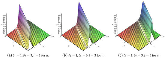
Figure 2. Solutions to Euler Equation (11) with Coriolis force.

Remark 2.

• We obtain the bell-shape single soliton solution to the Euler equation with Coriolis force. The vorticity (i.e., curl of the velocity) of the Euler flow is

  $$\Omega =curl(\mathbf{U})=\frac{\partial u}{\partial y}-\frac{\partial v}{\partial x}=-4\mathit{sec}{h}^2((v_1-v_2)t-x+y)\tanh ((v_1-v_2)t-x+y)\ne 0,$$

  which shows the Euler flow with Coriolis force is a rotational flow.
• Using Equation (24) as a seed solution, various invariant solutions can be given with $f^{(i)}(i=1,...,5)$ obtained in Section 3.2.

Case 2. $C_7=1.\mathrm{Let}{C}_6=C_i=0(i=8,\dots ,11),\beta (t)=0$.

From Equations (15), we have

$${\underline{V}}_2=C_7{\Delta }_t={\Delta }_t.$$

We get the invariants

$$\overline{\xi }=x,\overline{\eta }=y,u=F(\overline{\xi },\overline{\eta }),v=G(\overline{\xi },\overline{\eta }),\overline{\eta }),P=Q(\overline{\xi },\overline{\eta }).$$

Substituting the group invariants into Equations (11), we obtain the following reduction equations:

$$\left\{\begin{array}{c}{F}_{\overline{\eta }}{F}_{\overline{\xi }}+F{F}_{\overline{\xi }\overline{\eta }}+G_{\overline{\eta }}{F}_{\overline{\eta }}+G{F}_{\overline{\eta }\overline{\eta }}+Q_{\overline{\xi }\overline{\eta }}=2\omega (t)G_{\overline{\eta }},\hfill \\ F_{\overline{\xi }}{G}_{\overline{\xi }}+F{G}_{\overline{\xi }\overline{\xi }}+G_{\overline{\xi }}{G}_{\overline{\eta }}+G{G}_{\overline{\xi }\overline{\eta }}+Q_{\overline{\xi }\overline{\eta }}=-2\omega (t)F_{\overline{\xi }},\hfill \\ F_{\overline{\xi }}+G_{\overline{\eta }}=0.\hfill \end{array}\right.$$

(25)

If F depends on $\overline{\eta }$ and G depends on $\overline{\xi }$ only, the third equation of (25) is satisfied naturally, then Equations (25) can be further reduced as

$$F{G}_{\overline{\xi }\overline{\xi }}-G{F}_{\overline{\eta }\overline{\eta }}=0.$$

(26)

Solving Equations (26), the exact solutions to the Euler equation can be obtained. We give one form of exact solutions as follows:

$$u=\cos y,v=\cos x,P=\sin x\sin y+2\omega (t)\sin x-2\omega (t)\sin y.$$

(27)

Using Equation (27) as a seed solution, various invariant solutions can be given with $f^{(i)}(i=1,\dots ,5)$ obtained in Section 3.2, e.g.,

$$\left\{\begin{array}{c}u=\cos (y-t\epsilon )+\epsilon ,v=\cos (x-t\epsilon )+\epsilon ,\hfill \\ P=\sin (x-t\epsilon )\sin (y-t\epsilon )+2\omega (t)(x-y)\epsilon +2\omega (t)\sin (x-t\epsilon )-2\omega (t)\sin (y-t\epsilon ).\hfill \end{array}\right.$$

(28)

We give the respective Figure 3 to have a more intuitive understanding of the solution (28).

Figure 3. Solutions to Euler Equation (11) with Coriolis force.

Remark 3.

From the solution and respective figure, we can find the flow present periodic oscillation. Since the vorticity (i.e., curl of the velocity) of the Euler flow is

$$\Omega =\frac{\partial u}{\partial y}-\frac{\partial v}{\partial x}=\sin (t\epsilon -y)+\sin (t\epsilon -x)\ne 0,$$

this shows that the Euler flow with Coriolis force is a rotational flow with periodic oscillation.

4. Conclusions

As a powerful tool that can be used to derive the exact solutions for both continuous and discrete equations, the Lie symmetry analysis method to general dynamical system is generalized on a time scale. Based on the Leibnitz formula on a time scale, the symmetry analysis of the Burgers equation and Euler equation with Coriolis force on a time scale is investigated, and the single parameter groups are obtained. Some group invariant solutions in explicit form for the traffic flow model simulated by Burgers equation and Euler equation with Coriolis force on a time scale are studied. The study of Burgers equation and Euler equation also establishes a foundation for the further study of the closely related Navier–Stokes equation that was considered as a famous Millennium puzzle. The applications of the method to other dynamical equations on a time scale which possess practical meaning are worthy of further study.

References

- Bohner, M.; Peterson, A. Advances in Dynamic Equations on a Time Scale; Birkhauser: Boston, MA, USA, 2002. [Google Scholar]
- Bohner, M.; Peterson, A. Dynamic Equations on a Time Scale: An Introduction with Applications; Springer Science & Business Media: Berlin, Germany, 2012. [Google Scholar]
- Hilger, S. Analysis on measure chains—A unified approach to continuous and discrete calculus. Results Math. 1990, 18, 18–56. [Google Scholar] [CrossRef]
- Agarwal, R.P.; O’Regan, D. Triple solutions to boundary value problems on a time scale. Appl. Math. Lett. 2000, 13, 7–11. [Google Scholar] [CrossRef]
- Chyan, C.J. Uniqueness Implies Existence on Time Scales. J. Math. Anal. Appl. 2001, 258, 359–365. [Google Scholar] [CrossRef][Green Version]
- Peterson, A.C.; Tisdell, B.C.C. Boundedness and Uniqueness of Solutions to Dynamic Equations on Time Scales. J. Differ. Equ. Appl. 2004, 10, 1295–1306. [Google Scholar] [CrossRef]
- Hoffacker, J.; Tisdell, C.C. Stability and instability for dynamic equations on a time scale. Comput. Math. Appl. 2005, 49, 1327–1334. [Google Scholar] [CrossRef]
- Amster, P.; Rogers, C.; Tisdell, C.C. Existence of solutions to boundary value problems for dynamic systems on a time scale. J. Math. Anal. Appl. 2005, 308, 565–577. [Google Scholar] [CrossRef]
- Sun, H.; Li, W. Existence theory for positive solutions to one-dimensional p-Laplacian boundary value problems on a time scale. J. Differ. Equ. 2007, 240, 217–248. [Google Scholar] [CrossRef]
- Chen, H.; Wang, H.; Zhang, Q.; Zhou, T. Double positive solutions of boundary value problems for p-Laplacian impulsive functional dynamic equations on a time scale. Comput. Math. Appl. 2007, 53, 1473–1480. [Google Scholar] [CrossRef][Green Version]
- Zhang, J.; Fan, M.; Zhu, H. Existence and roughness of exponential dichotomies of linear dynamic equations on a time scale. Comput. Math. Appl. 2010, 59, 2658–2675. [Google Scholar] [CrossRef][Green Version]
- Federson, M.; Grau, R.; Mesquita, J.G.; Toon, E. Boundedness of solutions of measure differential equations and dynamic equations on a time scale. J. Differ. Equ. 2017, 263, 26–56. [Google Scholar] [CrossRef]
- Lou, S. Symmetry analysis and exact solutions of the (2+1)-dimensional sine-Gordon system. J. Math. Phys. 2000, 41, 6509–6524. [Google Scholar] [CrossRef]
- Tian, C. Lie Group and Its Application in Differential Equations; Science Press: Beijing, China, 2005. [Google Scholar]
- Liu, H.; Geng, Y. Symmetry reductions and exact solutions to the systems of carbon nanotubes conveying fluid. J. Differ. Equ. 2013, 254, 2289–2303. [Google Scholar] [CrossRef]
- Liu, H.; Li, J. Symmetry reductions, dynamical behavior and exact explicit solutions to the Gordon types of equations. J. Comput. Appl. Math. 2014, 257, 144–156. [Google Scholar] [CrossRef]
- Tiwari, A.K.; Pandey, S.N.; Senthilvelan, M.; Lakshmanan, M. Lie point symmetries classification of the mixed Liénard-type equation. Nonlinear Dynam. 2015, 82, 1953–1968. [Google Scholar] [CrossRef]
- Baleanu, D.; Inc, M.; Yusuf, A.; Aliyu, I.A. Lie symmetry analysis, exact solutions and conservation laws for the time fractional Caudrey-Dodd-Gibbon-Sawada-Kotera equation. Commun. Nonlinear Sci. 2018, 59, 222–234. [Google Scholar] [CrossRef]
- Burgers, J. The Nonlinear Diffusion Equation; Dordrecht: Amsterdam, The Netherlands, 1974. [Google Scholar]
- Smoller, J. Shock Waves and Reaction Diffusion Equations, 2nd ed.; Springer: Berlin, Germany, 1994. [Google Scholar]
- Biler, P.; Funaki, T.; Woyczynski, W.A. Fractal Burgers equations. J. Differ. Equ. 1998, 148, 9–46. [Google Scholar] [CrossRef]
- Pettersson, P.; Iaccarino, G.; Nordström, J. Numerical analysis of the Burgers’ equation in the presence of uncertainty. J. Comput. Phys. 2009, 228, 8394–8412. [Google Scholar] [CrossRef]
- Neate, A.; Truman, A. The stochastic Burgers equation with vorticity: Semiclassical asymptotic series solutions with applications. J. Math. Phys. 2011, 52, 185–383. [Google Scholar] [CrossRef]
- Heinz, S. Comments on a priori and a posteriori evaluations of sub-grid scale models for the Burgers’ equation. Comput. Fluids 2016, 138, 35–37. [Google Scholar] [CrossRef]
- Landau, L.D.; Lifshitz, E.M. Fluid Mechanics; Pergamon Press: New York, NY, USA, 1987. [Google Scholar]
- Majda, A.J.; Majda, A.J.; Bertozzi, A.L. Vorticity and Incompressible Flow; Cambridge University Press: Cambridge, UK, 2002. [Google Scholar]
- Jia, M.; Chen, L.; Lou, S.Y. Relation between the induced flow and the position of typhoon: Chanchu 2006. Chin. Phys. Lett. 2006, 23, 2878. [Google Scholar]
- Koh, Y.; Lee, S.; Takada, R. Strichartz estimates for the Euler equations in the rotational framework. J. Differ. Equ. 2014, 256, 707–744. [Google Scholar] [CrossRef]
- Olver, P.J. Applications of Lie Groups to Differential Equations, 2nd ed.; Graduate Tests in Mathematics; Springer: Berlin, Germany, 1993; Volume 107. [Google Scholar]
© 2019 by the authors. Licensee MDPI, Basel, Switzerland. This article is an open access article distributed under the terms and conditions of the Creative Commons Attribution (CC BY) license (http://creativecommons.org/licenses/by/4.0/).