Covering Graphs, Magnetic Spectral Gaps and Applications to Polymers and Nanoribbons

Abstract

In this article, we analyze the spectrum of discrete magnetic Laplacians (DML) on an infinite covering graph $\tilde{\mathbf{G}}\to \mathbf{G}=\tilde{\mathbf{G}}/\Gamma$ with (Abelian) lattice group $\Gamma$ and periodic magnetic potential $\tilde{\beta }$. We give sufficient conditions for the existence of spectral gaps in the spectrum of the DML and study how these depend on $\tilde{\beta }$. The magnetic potential can be interpreted as a control parameter for the spectral bands and gaps. We apply these results to describe the spectral band/gap structure of polymers (polyacetylene) and nanoribbons in the presence of a constant magnetic field.

1. Introduction

It is a well-known fact that the spectrum of Laplacians or, more generally, Schrödinger operators with periodic potentials, on Abelian coverings, have band structure. These properties of the Laplacians are discussed, e.g., in [1,2] and the references therein. The spectrum consists of a continuous part (which is the union of intervals or spectral bands separated by gaps) and a set of eigenvalues with infinite multiplicity. The spectrum is described in terms of a so-called Floquet (or Bloch) parameter. This parameter is the dual of the Abelian group acting on the structure. If two consecutive spectral bands of a bounded self-adjoint operator T do not overlap, then we say that the spectrum has a spectral gap, i.e., a maximal nonempty interval $(a,b)\subset [-\parallel T\parallel ,\parallel T\parallel ]$ that does not intersect the spectrum of the operator. The study of the spectral bands/gaps is a quite natural situation in several fields of mathematics and physics. In solid-state physics, where—for example in semiconductors or its optical counterparts, photonic crystals—the operators modeling the dynamics of particles have some forbidden energy regions (see, e.g., [3,4]). In band-gap engineering, a process to control de band/gap of some materials, for semiconductors is controlled for example with the composition of alloys [5], and for the nanoribbons with temperature [6], etc. Depending on the type of the periodic structure involved, spectral gaps may be produced by deformation of the geometry (cf., [7,8,9]) or by a suitable periodic decoration of the metric or the discrete covering graph (see, e.g., [10,11,12,13,14] and ([15], Section 4)).

The study of energy-gaps has been widely studied. The gaps in nanoribbons as a function of the width can be found in [16]. The gaps in the armchair structure can appear because quantum confinement and for the zigzag structure can appear because of an edge magnetization [17].

In this article, we study the spectrum of discrete magnetic Laplacians (DMLs for short) on infinite discrete coverings graphs

$$\pi :\tilde{\mathbf{G}}\to \mathbf{G}=\tilde{\mathbf{G}}/\Gamma ,$$

where $\Gamma$ is an (Abelian) lattice group acting freely and transitively on $\tilde{\mathbf{G}}$ (also the graph $\tilde{\mathbf{G}}$ is called as $\Gamma$-periodic graph with finite quotient $\mathbf{G}$). We will present our analysis for graphs with arbitrary weights m on vertices and arcs although the graphs presented in the examples of the last section will initially have standard weights which are more usual in the context of mathematical physics. Also, we consider a periodic magnetic potential $\tilde{\beta }$ on the arcs of the covering graph $\tilde{\mathbf{G}}$ modeling a magnetic field acting on the graph.

We denote a weighted graph as $\mathbf{W}=(\mathbf{G},m)$, and a magnetic weighted graph (MW-graph for short) is a weighted graph $\mathbf{W}$ together with a magnetic potential acting on its arcs. Any MW-graph $\mathbf{W}=(\mathbf{G},m)$ with magnetic potential $\beta$ has canonically associated a DML denoted as ${\Delta }_{\beta }^{\mathbf{W}}$. We say that $\tilde{\mathbf{W}}=(\tilde{\mathbf{G}},\tilde{m})$ with magnetic potential $\tilde{\beta }$ is a $\Gamma$-periodic MW-graph if $\tilde{\mathbf{G}}\to \mathbf{G}=\tilde{\mathbf{G}}/\Gamma$ is a $\Gamma$-covering and $\tilde{m}$ and $\tilde{\beta }$ are periodic with respect to the group action.

In this article, we generalize the geometric condition obtained in ([18], Theorem 4.4) for $\tilde{\beta }=0$ to non-trivial periodic magnetic potentials. In particular, if $\tilde{\mathbf{W}}=(\tilde{\mathbf{G}},\tilde{m})$ is a $\Gamma$-periodic MW-graph with magnetic potential $\tilde{\beta }$, we will give in Theorem 3 a simple geometric condition on the quotient graph $\mathbf{G}=\tilde{\mathbf{G}}/\Gamma$ that guarantees the existence of non-trivial spectral gaps on the spectrum of the discrete magnetic Laplacian ${\Delta }_{\tilde{\beta }}^{\tilde{\mathbf{W}}}$. To show the existence of spectral gaps, we develop a purely discrete spectral localization technique based on the virtualization of arcs and vertices on quotient $\mathbf{G}$. These operations produce new graphs with, in general, different weights that allow localizing the eigenvalues of the original Laplacian inside certain intervals. We call this procedure discrete bracketing, and we refer to [18] for additional motivation and proofs.

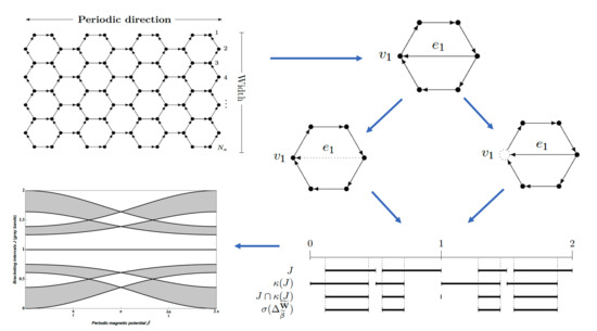
One of the new aspects of the present article is the generalization of results in [18] to include a periodic magnetic field $\tilde{\beta }$ on the covering graph $\pi :\tilde{\mathbf{G}}\to \mathbf{G}=\tilde{\mathbf{G}}/\Gamma$. In this sense, $\tilde{\beta }$ may be used as a control parameter for the system that serves to modify the size and the regions where the spectral gaps are localized. We apply our techniques to the graphs modeling the polyacetylene polymer as well as to graphene nanoribbons. The nanoribbons are $\mathbb{Z}$-periodic strips of graphene either with an armchair or zig-zag boundaries (see, e.g., Figure 5). The graphic in Figure 1 corresponds to an armchair nanoribbon with a width 3. It can be seen how a periodic magnetic potential with constant value $\tilde{\beta }\in [0,2\pi )$ on each cycle (and plotted on the horizontal axis) affects the spectral bands (gray vertical intervals that appear as the intersection of the region with a line $\tilde{\beta }=const$) and the spectral gaps (white vertical intervals). We refer to Section 5.2 for additional details of the construction.

In the case of the polyacetylene polymer, we find a spectral gap that is stable under perturbation of the (constant) magnetic field. Moreover, if the value of the magnetic field is $\pi$, then the spectrum of the DML degenerates to four eigenvalues of infinite multiplicity. This discrete model suggests that a varying uniform magnetic field may drastically change the conductance of a material arranged as a periodic planar graph.

The article is structured in five sections as follows. In Section 2, we collect the basic definitions and results on discrete weighted multigraphs (graphs which may have loops and multiple arcs). We consider discrete magnetic potentials on the arcs and define the discrete magnetic Laplacian on the graph, which will be the central operator in this work. In Section 3, we present a spectral relation between finite MW-graphs based on an order relation between the eigenvalues of the corresponding DMLs. Moreover, we will present the basic arc and vertex virtualization procedure that will allow one to localize the spectrum of the DML on the infinite covering graph. In Section 4, we extend the discrete Floquet theory considered in ([18], Section 5) to the case of covering graphs with periodic magnetic potentials. In Section 5, we apply the spectral localization results developed before in the example of $\mathbb{Z}$-periodic graphs modeling the polyacetylene polymer as well as graphene nanoribbons in the presence of a constant magnetic field.

2. Weighted Graphs and Discrete Magnetic Laplacians

In this section, we introduce the basic definitions and results concerning MW-graphs and also define discrete magnetic Laplacians. For further motivation and results, we refer to [12,18,19] and references cited therein.

We denote by $\mathbf{G}=\left(V,E,\partial \right)$ a (discrete) directed multigraph which in the following we call simply a graph; here $V=V(\mathbf{G})$ is the set of vertices and $E=E(\mathbf{G})$ the set of arcs. The orientation map is given by $\partial :E\to V\times V$ and $\partial e=\left({\partial }_{-}e,{\partial }_{+}e\right)$ is the pair of the initial and terminal vertices. Graphs are allowed to have multiple arcs, i.e., arcs $e_1\ne e_2$ with $\left({\partial }_{-}{e}_1,{\partial }_{+}{e}_1\right)=\left({\partial }_{-}{e}_2,{\partial }_{+}{e}_2\right)$ or $\left({\partial }_{-}{e}_1,{\partial }_{+}{e}_1\right)=\left({\partial }_{+}{e}_2,{\partial }_{-}{e}_2\right)$ as well as loops, i.e., arcs $e_1$ with ${\partial }_{-}{e}_1={\partial }_{+}{e}_1$. Moreover, we define

$$E_v:=E_v^{+}⊍E_v^{-}(\mathrm{disjoint}\mathrm{union}),\mathrm{where}{E}_v^{\pm }:=\left\{e\in E\mid v={\partial }_{\pm }e\right\}.$$

With this notation, the degree of a vertex is $\mathrm{deg}(v)=|E_v|$ and a loop increases the degree by 2.

Given subsets $A,B\subset V$, we define

$$E^{+}(A,B):=\left\{e\in E\mid {\partial }_{-}e\in A,{\partial }_{+}e\in B\right\}\mathrm{and}{E}^{-}(A,B):=E^{+}(B,A).$$

Moreover, we put $E(A,B):=E^{+}(A,B)\cup E^{-}(A,B)$ and $E(A):=E(A,A)$.

To simplify the notation, we write $E(v,w)$ instead of $E(\{v\},\{w\})$ etc. Note that loops are not counted double in $E(A,B)$, in particular, $E(v):=E(v,v)$ is the set of loops based at the vertex $v\in V$. The Betti number $b(\mathbf{G})$ of a finite graph $\mathbf{G}=\left(V,E,\partial \right)$ is defined as

$$b(\mathbf{G}):=\left|E\right|-\left|V\right|+1.$$

(1)

To study the virtualization processes of vertices, arcs and the structure of covering graphs, we will need to introduce the following substructures of a graph.

Definition 1.

Let $\mathbf{G}=(V,E,\partial )$ be a graph and denote by $\mathbf{H}=(V_0,E_0,{\partial }_0)$ a triple such that $V_0\subset V$, $E_0\subset E$ and ${\partial }_0=\partial {\upharpoonright }_{E_0}$.

(a) 

If $E_0\cap E(V\backslash V_0)=\varnothing$, we say that $\mathbf{H}$ is a partial subgraph in $\mathbf{G}$. We call

$$\begin{array}{cc}\hfill B(\mathbf{H},\mathbf{G}):=& E(V_0,V\backslash V_0)\hfill \\ \hfill =& \left\{e\in E\mid {\partial }_{-}e\in V_0,{\partial }_{+}e\in V\backslash V_{0}or{\partial }_{+}e\in V_0,{\partial }_{-}e\in V\backslash V_0\right\}\hfill \end{array}$$

(2)

the set of connecting arcs of the partial subgraph $\mathbf{H}$ in $\mathbf{G}$.

(b) 

If $E_0\subset E(V_0)$, then $\mathbf{H}$ is a subgraph of $\mathbf{G}$

Note that, in general, a partial subgraph $\mathbf{H}=(V_0,E_0,{\partial }_0)$ is not a graph as defined above, since we may have arcs $e\in E$ with ${\partial }_{\pm }e\notin V_0$. We do exclude though the case that ${\partial }_{+}e\notin V_0$ and ${\partial }_{-}e\notin V_0$. The arcs not mapped into $V_0\times V_0$ under ${\partial }_0$ are precisely the connecting arcs of $\mathbf{H}$ in $\mathbf{G}$. Partial subgraphs appear naturally as fundamental domains of covering graphs (cf., Section 4) (Note that we use the name partial subgraph in a different sense as in usual combinatorics literature).

Let $\mathbf{G}=(V,E,\partial )$ be a graph; a weight on $\mathbf{G}$ is a pair of functions denoted by a unique symbol m on the vertices and arcs $m:V\to (0,\infty )$ and $m:E\to (0,\infty )$ such that $m(v)$ is the weight at the vertex v and $m_e$ is the weight at $e\in E$. We call $\mathbf{W}=(\mathbf{G},m)$ a weighted graph. It is natural to interpret m as a positive measure and consider $m(E_0):={\sum }_{e\in E_0}{m}_e$ for any $E_0\subset E$. The relative weight is $\rho :V\to (0,\infty )$ defined as

$$\rho (v):={\displaystyle \frac{m(E_v)}{m(v)}}={\displaystyle \frac{m(E_v^{+})+m(E_v^{-})}{m(v)}}.$$

(3a)

In order to work with bounded discrete magnetic Laplacians, we will assume that the relative weight is uniformly bounded, i.e.,

$${\rho }_{\infty }:=\underset{v\in V}{\sup }\rho (v)<\infty .$$

(3b)

The most important and intrinsic examples of weights are

• Standard weight:$m(v)=\mathrm{deg}(v)$, $v\in V$, and $m_e=1$, $e\in E$, so that $\rho (v)={\rho }_{\infty }=1$.
• Combinatorial weight:$m(v)=m_e=1$, $v\in V$, $e\in E$ hence $\rho (v)=\mathrm{deg}(v)$ and ${\rho }_{\infty }={\sup }_{v\in V}\mathrm{deg}(v)$.

Giving a weighted graph $\mathbf{W}=(\mathbf{G},m)$, we associate the following two natural Hilbert spaces which we interpret as 0-forms and 1-forms, respectively.

$$\begin{array}{cc}\hfill {\ell }_2(V,m)& :=\left\{f:V\to \mathbb{C}\mid {∥f∥}_{V,m}^2=\sum _{v\in V}{\left|f(v)\right|}^{2}m(v)<\infty \right\}\mathrm{and}\hfill \\ \hfill {\ell }_2(E,m)& :=\left\{\eta :E\to \mathbb{C}\mid {∥\eta ∥}_{E,m}^2=\sum _{e\in E}{\left|{\eta }_e\right|}^2{m}_e<\infty \right\},\hfill \end{array}$$

with corresponding inner products

$${〈f,g〉}_{{\ell }_2(V,m)}=\sum _{v\in V}f(v)\overline{g(v)}m(v)\mathrm{and}{〈\eta ,\zeta 〉}_{{\ell }_2(E,m)}=\sum _{e\in E}{\eta }_e\overline{{\zeta }_e}{m}_e.$$

Let $\mathbf{G}$ be a graph; a magnetic potential$\alpha$ acting on $\mathbf{G}$ is a $\mathbb{T}$-valued function on the arcs as follows, $\alpha :E(\mathbf{G})\to \mathbb{T}=\mathbb{R}/2\pi \mathbb{Z}.$ We denote the set of all vector potentials on $E(\mathbf{G})$ just by $\mathcal{A}(\mathbf{G})$. We say that two magnetic potentials ${\alpha }_1$ and ${\alpha }_2$ are cohomologous, and denote this as ${\alpha }_1\sim {\alpha }_2$, if there is $\phi :V\to \mathbb{T}$ with

$${\alpha }_1={\alpha }_2+d\phi .$$

Given a $E_0\subset E(\mathbf{G})$, we say that a magnetic potential $\alpha$ has support in $E_0$ if ${\alpha }_e=0$ for all $e\in E(\mathbf{G})\backslash E_0$. We call the class of weighted graphs with magnetic potential MW-graphs for short.

It can be shown that any magnetic potential on a finite graph can be supported in $b(\mathbf{G})$ many arcs. For example, if $\mathbf{G}$ is a cycle, any magnetic potential is cohomologous to a magnetic potential supported in only one arc. Moreover, if $\mathbf{G}$ is a tree, any magnetic potential acting on $\mathbf{G}$ is cohomologous to 0.

The twisted (discrete) derivative is the following linear operator mapping 0-forms into 1-forms:

$$d_{\alpha }:{\ell }_2(V,m)\to {\ell }_2(E,m)\mathrm{with}{\left(d_{\alpha }f\right)}_e={\mathrm{e}}^{\mathrm{i}{\alpha }_e/2}f({\partial }_{+}e)-{\mathrm{e}}^{-\mathrm{i}{\alpha }_e/2}f({\partial }_{-}e).$$

(4)

Now, we present the following geometrical definition of Laplacian with magnetic field as a generalization of the discrete Laplace-Beltrami operator.

Definition 2.

Let $\mathbf{W}=(\mathbf{G},m)$ be a weighted graph with $\alpha :E\to \mathbb{T}$ a vector potential. The discrete magnetic Laplacian (DML for short) ${\Delta }_{\alpha }:{\ell }_2(V)\to {\ell }_2(V)$ is defined by ${\Delta }_{\alpha }=d_{\alpha }^{*}{d}_{\alpha }$, i.e., by

$$\left({\Delta }_{\alpha }f\right)\left(v\right)=\rho (v)f(v)-{\displaystyle \frac{1}{m(v)}}\sum _{e\in E_v}{\mathrm{e}}^{\mathrm{i}{\stackrel{\curvearrowright }{\alpha }}_e(v)}f(v_e)m_e,$$

where ${\stackrel{\curvearrowright }{\alpha }}_e(v)$ is the oriented evaluation and $v_e$ is the vertex opposite to v along the arc e, i.e.,

$${\stackrel{\curvearrowright }{\alpha }}_e(v)=\left\{\begin{array}{cc}-{\alpha }_e,\hfill & \mathit{if}v={\partial }_{-}e,\hfill \\ {\alpha }_e,\hfill & \mathit{if}v={\partial }_{+}e,\hfill \end{array}\right.\mathit{and}{v}_e=\left\{\begin{array}{cc}{\partial }_{+}e,\hfill & \mathit{if}v={\partial }_{-}e,\hfill \\ {\partial }_{-}e\hfill & \mathit{if}v={\partial }_{+}e.\hfill \end{array}\right.$$

If we need to stress the dependence of the operator of the weighted graph $\mathbf{W}=(\mathbf{G},m)$, we will denote the DML as ${\Delta }_{\alpha }^{\mathbf{W}}$.

From this definition, it follows immediately that the DML ${\Delta }_{\alpha }$ is a bounded, positive and self-adjoint operator. Its spectrum satisfies $\sigma ({\Delta }_{\alpha })\subset [0,2{\rho }_{\infty }]$ and, in contrast to the usual Laplacian without magnetic potential, the DML depends on the orientation of the graph. If $\alpha \sim {\alpha }^{\prime }$, then ${\Delta }_{\alpha }$ and ${\Delta }_{{\alpha }^{\prime }}$ are unitary equivalent; in particular, $\sigma ({\Delta }_{\alpha })=\sigma ({\Delta }_{{\alpha }^{\prime }})$. Moreover, if $\alpha \sim 0$ then ${\Delta }_{\alpha }\cong \Delta$ where $\Delta$ denotes the usual discrete Laplacian (with vector potential 0). For example, if $\mathbf{W}=(\mathbf{G},m)$ and $\mathbf{G}$ is a tree, then ${\Delta }_{\alpha }^{\mathbf{W}}\cong {\Delta }^{\mathbf{W}}$ for any magnetic potential $\alpha$.

3. Spectral Ordering on Finite Graphs and Magnetic Spectral Gaps

In this section, we will introduce a spectral ordering relation ≼, which is invariant under unitary equivalence of the corresponding operators. Moreover, we will introduce two operations on the graphs (virtualization of arcs and vertices) that will be used later to develop a spectral localization (bracketing) of DML on finite graphs. This technique will finally be applied to discuss the existence of spectral gaps for magnetic Laplacians on covering graphs. We refer to [11,12,18] for additional motivation and examples. For proofs of the results stated in this section see ([18], Sections 3 and 4).

Let $\mathbf{W}=(\mathbf{G},m)$ be a weighted graph. Throughout this section, we will assume that $|V(\mathbf{G})|=n<\infty$. We denote the spectrum of the DML by $\sigma ({\Delta }_{\alpha }^{\mathbf{W}}):=\{{\lambda }_k({\Delta }_{\alpha }^{\mathbf{W}})\mid k=1,\dots ,n\}\subset [0,2{\rho }_{\infty }]$, where we will write the eigenvalues in ascending order and repeated according to their multiplicities, i.e.,

$$0\le {\lambda }_1({\Delta }_{\alpha }^{\mathbf{W}})\le {\lambda }_2({\Delta }_{\alpha }^{\mathbf{W}})\le \cdots \le {\lambda }_n({\Delta }_{\alpha }^{\mathbf{W}}).$$

Definition 3.

Let ${\mathbf{W}}^{-}$ and ${\mathbf{W}}^{+}$ be two finite MW-graphs of order $n^{-}$ and $n^{+}$, respectively, and magnetic potential ${\alpha }^{\pm }$. Consider the eigenvalues of the DMLs ${\Delta }_{\alpha }^{{\mathbf{W}}^{\pm }}$ written in ascending order and repeated according to their multiplicities.

(a) 

We say that ${\mathbf{W}}^{-}$ is spectrally smaller than ${\mathbf{W}}^{+}$ (denoted by ${\mathbf{W}}^{-}\preccurlyeq {\mathbf{W}}^{+}$), if

$$n^{-}\ge n^{+}\mathit{and}\mathit{if}{\lambda }_k({\Delta }_{{\alpha }^{-}}^{{\mathbf{W}}^{-}})\le {\lambda }_k({\Delta }_{{\alpha }^{+}}^{{\mathbf{W}}^{+}})\mathit{for}\mathit{all}1\le k\le n^{-},$$

where we put ${\lambda }_k({\Delta }_{{\alpha }^{+}}^{{\mathbf{W}}^{+}}):=2{\rho }_{\infty }$ for $k=n^{+}+1,\dots ,n^{-}$ (the maximal possible eigenvalue).

(b) 

Consider ${\mathbf{W}}^{\pm }$ as above with ${\mathbf{W}}^{-}\preccurlyeq {\mathbf{W}}^{+}$. We define the associated k-th bracketing interval $J_k=J_k({\mathbf{W}}^{-},{\mathbf{W}}^{+})$ by

$$J_k:=\left[{\lambda }_k({\Delta }_{{\alpha }^{-}}^{{\mathbf{W}}^{-}}),{\lambda }_k({\Delta }_{{\alpha }^{+}}^{{\mathbf{W}}^{+}})\right]$$

(5)

for $k=1,\dots ,n^{-}$.

Given an MW-graph, we introduce two elementary operations that consist of virtualizing arcs and vertices. The first one will lead to a spectrally smaller graph.

Definition 4

(virtualizing arcs). Let $\mathbf{W}=(\mathbf{G},m)$ be a weighted graph with magnetic potential α and $E_0\subset E(\mathbf{G})$. We denote by ${\mathbf{W}}^{-}=({\mathbf{G}}^{-},m^{-})$ the weighted subgraph with magnetic potential ${\alpha }^{-}$ defined as follows:

(a) 

$V({\mathbf{G}}^{-})=V(\mathbf{G})$ with $m^{-}(v):=m(v)$ for all $v\in V(\mathbf{G})$;

(b) 

$E({\mathbf{G}}^{-})=E(\mathbf{G})\backslash E_0$ with $m_e^{-}:=m_e$ and ${\partial }_{\pm }^{{\mathbf{G}}^{-}}e={\partial }_{\pm }^{\mathbf{G}}e$ for all $e\in E({\mathbf{G}}^{-})$;

(c) 

${\alpha }_e^{-}={\alpha }_e$, $e\in E({\mathbf{G}}^{-})$.

We call ${\mathbf{W}}^{-}$ the weighted subgraph obtained from $\mathbf{W}$ by virtualizing the arcs $E_0$. We will sometimes denote the weighted graph simply by ${\mathbf{W}}^{-}=\mathbf{W}-E_0$ and we write the corresponding discrete magnetic Laplacian as ${\Delta }_{{\alpha }^{-}}^{{\mathbf{W}}^{-}}$.

The second elementary operation on the graph will lead now to a spectrally larger graph.

Definition 5

(virtualizing vertices). Let $\mathbf{W}=(\mathbf{G},m)$ be a weighted graph with magnetic potential α and $V_0\subset V(\mathbf{G})$. We denote by ${\mathbf{W}}^{+}=({\mathbf{G}}^{+},m^{+})$ the weighted partial subgraph with magnetic potential ${\alpha }^{+}$ defined as follows:

(a) 

$V({\mathbf{G}}^{+})=V(\mathbf{G})\backslash V_0$ with $m^{+}(v):=m(v)$ for all $v\in V({\mathbf{G}}^{+})$;

(b) 

$E({\mathbf{G}}^{+})=E(\mathbf{G})\backslash {\bigcup }_{v_0\in V_0}E(v_0)$ with $m_e^{+}=m_e$ for all $e\in E(\mathbf{G})$;

(c) 

${\alpha }_e^{+}={\alpha }_e$, $e\in E({\mathbf{G}}^{+})$.

We call ${\mathbf{W}}^{+}$ the weighted partial subgraph obtained from $\mathbf{W}$ by virtualizing the vertices $V_0$. We will denote it simply by ${\mathbf{W}}^{+}=\mathbf{W}-V_0$. The corresponding discrete magnetic Laplacian is defined by

$${\Delta }_{{\alpha }^{+}}^{{\mathbf{W}}^{+}}={(d_{{\alpha }^{+}})}^{*}{d}_{{\alpha }^{+}},\mathit{where}{d}_{{\alpha }^{+}}:=d_{\alpha }\circ \iota$$

with

$$\iota :{\ell }_2(V({\mathbf{G}}^{+}),m^{+})\to {\ell }_2(V(\mathbf{G}),m),(\iota f)(v)=\left\{\begin{array}{cc}f(v),\hfill & v\in V({\mathbf{G}}^{+}),\hfill \\ 0,\hfill & v\in V_0.\hfill \end{array}\right.$$

It can be shown that the operator ${\Delta }_{{\alpha }^{+}}^{{\mathbf{W}}^{+}}$ is the compression of ${\Delta }^{\mathbf{W}}$ onto a $(|V|-|V_0|)$-subspace.

The previous operations of arc and vertex virtualization will be used to localize the spectrum of intermediate DMLs. Before summarizing the technique in the next theorem, we need to introduce the following notion of vertex neighborhood of a family of arcs.

Definition 6.

Let $\mathbf{G}$ be a graph and $E_0\subset E(\mathbf{G})$. We say that a vertex subset $V_0\subset V(\mathbf{G})$ is in the neighborhood of $E_0$if $E_0\subset {\bigcup }_{v\in V_0}{E}_v$, i.e., if ${\partial }_{+}e\in V_0$ or ${\partial }_{-}e\in V_0$ for all $e\in E_0$.

Later on, $E_0$ will be the set of connecting arcs of a covering graph, and we will choose $V_0$ to be as small as possible to guarantee the existence of spectral gaps (this set is in general not unique).

Theorem 1.

Let $\mathbf{W}=(\mathbf{G},m)$ be a finite MW-graph with magnetic potential α and $E_0\subset E(\mathbf{G})$. Then, for any subset of vertices $V_0$ in a neighborhood of $E_0$ we have

$${\mathbf{W}}^{-}\preccurlyeq \mathbf{W}\preccurlyeq {\mathbf{W}}^{+},$$

(6)

where ${\mathbf{W}}^{-}=({\mathbf{G}}^{-},m^{-})$ with ${\mathbf{G}}^{-}=\mathbf{G}-E_0$ and ${\mathbf{W}}^{+}=({\mathbf{G}}^{+},m^{+})$ with ${\mathbf{G}}^{+}=\mathbf{G}-V_0$. In particular, we have the spectral localizing inclusion

$$\sigma ({\Delta }_{\alpha }^{\mathbf{W}})\subset J:=J({\mathbf{W}}^{-},{\mathbf{W}}^{+})=\bigcup _{k=1}^{|V(\mathbf{G})|}\left[{\lambda }_k({\Delta }_{{\alpha }^{-}}^{{\mathbf{W}}^{-}}),{\lambda }_k({\Delta }_{{\alpha }^{+}}^{{\mathbf{W}}^{+}})\right];.$$

(7)

By construction, it is clear that the bracketing $J=J(\alpha )$ depends on the magnetic potential $\alpha$. In Section 5, we show in some examples how the localization intervals $J_k$ change under the variation of the magnetic potential (see, e.g., Figure 3). However, if the magnetic potential $\alpha$ has support on the virtualized arcs $E_0$, then J will not depend on $\alpha$ because ${\alpha }^{\pm }\sim 0$.

Next, we make precise some notions concerning spectral gaps that will be needed when we study covering graphs. Recall that $\sigma ({\Delta }_{\alpha }^{\mathbf{G}})\subset [0,2{\rho }_{\infty }]$, where ${\rho }_{\infty }$ denotes the supremum of the relative weight, (cf., Equation (3)).

Definition 7.

Let $\mathbf{W}=(\mathbf{G},m)$ be a weighted graph.

(a) 

The spectral gaps set of $\mathbf{W}$ is defined by

$${\mathcal{S}}^{\mathbf{W}}=[0,2{\rho }_{\infty }]\backslash \sigma ({\Delta }^{\mathbf{W}})=[0,2{\rho }_{\infty }]\cap \rho ({\Delta }^{\mathbf{W}}),$$

where $\rho ({\Delta }^{\mathbf{W}})$ denotes the resolvent set of the operator ${\Delta }^{\mathbf{W}}$.

(b) 

The magnetic spectral gaps set of $\mathbf{W}$ is defined by

$${\mathcal{MS}}^{\mathbf{W}}=[0,2{\rho }_{\infty }]\backslash \bigcup _{\alpha \in \mathcal{A}(\mathbf{G})}\sigma ({\Delta }_{\alpha }^{\mathbf{W}})=\bigcap _{\alpha \in \mathcal{A}(\mathbf{G})}\rho ({\Delta }_{\alpha }^{\mathbf{W}})\cap [0,2{\rho }_{\infty }].$$

where the union is taken over all the magnetic potential α acting on $\mathbf{G}$.

The following elementary properties follow directly from the definition: ${\mathcal{MS}}^{\mathbf{W}}\subset {\mathcal{S}}^{\mathbf{W}}$. In particular, if ${\mathcal{S}}^{\mathbf{W}}=\varnothing$, then ${\mathcal{MS}}^{\mathbf{W}}=\varnothing$ or, equivalently, if ${\mathcal{MS}}^{\mathbf{W}}\ne \varnothing$, then ${\mathcal{S}}^{\mathbf{W}}\ne \varnothing$. Moreover, if $\mathbf{G}$ is a tree, then ${\mathcal{MS}}^{\mathbf{W}}={\mathcal{S}}^{\mathbf{W}}$, as all DMLs are unitary equivalent with the usual Laplacian ${\Delta }^{\mathbf{W}}$.

Up to now, we have seen that arc/vertex virtualization will produce graphs ${\mathbf{W}}^{\pm }$ that allows localizing the spectrum of the DML of any intermediate MW-graph $\mathbf{W}$ satisfying

$${\mathbf{W}}^{-}\preccurlyeq \mathbf{W}\preccurlyeq {\mathbf{W}}^{+}.$$

4. Periodic Graphs and Spectral Gaps

In this section, we will study the spectrum of the DML of an infinite covering graph with periodic magnetic potential in terms of its Floquet decomposition. In Proposition 2 the Floquet parameter of the covering graph is identified with a suitable set of magnetic potentials $\alpha$ on the quotient (cf., Definition 10). This approach generalizes results in ([18], Section 5) to include Laplacians on the infinite covering graph with a periodic magnetic potential $\tilde{\beta }$. Finally, in Theorem 2, we state a bracketing technique to localize the spectrum.

4.1. Periodic Graphs and Fundamental Domains

Let $\Gamma$ be an (Abelian) lattice group and consider the $\Gamma$-covering (or $\Gamma$-periodic) graph

$$\pi :\tilde{\mathbf{G}}\to \mathbf{G}=\tilde{\mathbf{G}}/\Gamma .$$

We assume that $\Gamma$ acts freely and transitively on the connected graph $\tilde{\mathbf{G}}$ with finite quotient $\mathbf{G}=\tilde{\mathbf{G}}/\Gamma$ (see also ([20], Chapters 5 and 6) or [18,21]). This action (which we write multiplicatively) is orientation preserving, i.e., $\Gamma$ acts both on $\tilde{V}$ and $\tilde{E}$ such that

$${\partial }_{+}(\gamma e)=\gamma ({\partial }_{+}e)\mathrm{and}{\partial }_{-}(\gamma e)=\gamma ({\partial }_{-}e)\mathrm{for}\mathrm{all}\gamma \in \Gamma \mathrm{and}e\in \tilde{E}.$$

In particular, we have ${\tilde{E}}_{\gamma v}=\gamma {\tilde{E}}_v$, $\gamma \in \Gamma$, $v\in \tilde{V}$.

In addition, we will study weighted covering graphs with a periodic weight $\tilde{m}$ and periodic magnetic potential $\tilde{\beta }$, i.e., we consider $\tilde{\mathbf{W}}=(\tilde{\mathbf{G}},\tilde{m},\tilde{\beta })$ an MW-graph such that for any $\gamma \in \Gamma$ we have

$$\tilde{m}(\gamma v)=\tilde{m}(v),v\in \tilde{V},{\tilde{m}}_{\gamma e}={\tilde{m}}_e,e\in \tilde{E}\mathrm{and}{\tilde{\beta }}_{\gamma e}={\tilde{\beta }}_e,e\in \tilde{E}.$$

Note that, by definition, the standard or combinatorial weights on a covering graph satisfy the invariance conditions on the weights. A $\Gamma$-covering weighted graph $\tilde{\mathbf{W}}=(\tilde{\mathbf{G}},\tilde{m})$ naturally induces a weight m and a magnetic potential $\beta$ on the quotient graph $\mathbf{G}=\tilde{\mathbf{G}}/\Gamma$, given by $m=\tilde{m}\circ {\pi }^{-1}$ and $\beta =\tilde{\beta }\circ {\pi }^{-1}$.

We define next some useful notions in relation to covering graphs (see, e.g., [18], Section 5 as well as ([22], Sections 1.2 and 1.3) and [8]).

Definition 8.

Let $\tilde{\mathbf{G}}=(\tilde{V},\tilde{E},\tilde{\partial })$ be a Γ-covering graph.

(a) 

a vertex, respectively arc fundamental domain on a Γ-covering graph is given by two subsets $D^V\subset \tilde{V}$ and $D^E\subset \tilde{E}$ satisfying

$$\begin{array}{cc}\hfill \tilde{V}& =\bigcup _{\gamma \in \Gamma }\gamma D^V\mathit{and}{\gamma }_1{D}^V\cap {\gamma }_2{D}^V=\varnothing \mathit{if}{\gamma }_1\ne {\gamma }_2,\hfill \\ \hfill \tilde{E}& =\bigcup _{\gamma \in \Gamma }\gamma D^E\mathit{and}{\gamma }_1{D}^E\cap {\gamma }_2{D}^E=\varnothing \mathit{if}{\gamma }_1\ne {\gamma }_2\hfill \end{array}$$

with $D^E\cap E(\tilde{V}\backslash D^V)=\varnothing$ (i.e., an arc in $D^E$ has at least one endpoint in $D^V$). We often simply write D for a fundamental domain, where D stands either for $D^V$ or $D^E$.

(b) 

a (graph) fundamental domain of a covering graph $\tilde{\mathbf{G}}$ is a partial subgraph (cf., Definition 1)

$$\mathbf{H}=(D^V,D^E,\partial {\upharpoonright }_{D^E}),$$

where $D^V$ and $D^E$ are vertex and arc fundamental domains, respectively. We call

$$B(\mathbf{H},\tilde{\mathbf{G}}):=E(D^V,V\backslash D^V)$$

the set of connecting arcs of the fundamental domain $\mathbf{H}$ in $\tilde{\mathbf{G}}$.

Remark 1.

(a) 

Fixing a fundamental domain on the covering graph and the group Γ will be used to give coordinates (to the arcs and vertices) on the covering graph $\tilde{\mathbf{G}}$.

In fact, given a specific fundamental domain $D^V$ in a Γ-covering graph $\tilde{\mathbf{G}}$, we can write any $v\in V(\tilde{\mathbf{G}})$ uniquely as $v=\xi (v)v_0$ for a unique pair $(\xi (v),v_0)\in \Gamma \times D^V$. This observation follows from the fact that the action is free and transitive. We call $\xi (v)$ the Γ-coordinate of v (with respect to the fundamental domain $D^V$). Similarly, we can define the coordinates for the arcs: any $e\in E(\tilde{\mathbf{G}})$ can be written as $e=\xi (e)e_0$ for a unique pair $(\xi (e),e_0)\in \Gamma \times D^E$. In particular, we have

$$\xi (\gamma v)=\gamma \xi (v)\mathit{and}\xi (\gamma e)=\gamma \xi (e),\mathit{for}\mathit{all}\gamma \in \Gamma .$$

(b) 

Once we have chosen a fundamental domain $\mathbf{H}=(D^V,D^E,\partial )$, we can embed $\mathbf{H}$ into the quotient $\mathbf{G}=\tilde{\mathbf{G}}/\Gamma$ of the covering $\pi :\tilde{\mathbf{G}}\to \mathbf{G}=\tilde{\mathbf{G}}/\Gamma$ by

$$D^V\to V(\mathbf{G})=V/\Gamma ,v\mapsto \left[v\right]\mathit{and}{D}^E\to E(\mathbf{G})=E/\Gamma ,e\mapsto \left[e\right],$$

where $\left[v\right]$ and $\left[e\right]$ denote the Γ-orbits of v and e, respectively. By definition of a fundamental domain, these maps are bijective. Moreover, if ${\partial }_{\pm }e=v$ in $\mathbf{H}$, then also ${\partial }_{\pm }(\left[e\right])=\left[v\right]$ in $\mathbf{G}$, i.e., the embedding is a (partial) graph homomorphism.

Definition 9.

Let $\tilde{\mathbf{G}}=(\tilde{V},\tilde{E},\partial )$ be a Γ-covering graph with fundamental graph $\mathbf{H}=(D^V,D^E,\partial )$. We define the index of an arc $e\in \tilde{E}$ as

$${\mathrm{ind}}_{\mathbf{H}}(e):=\xi ({\partial }_{+}e){\left(\xi ({\partial }_{-}e)\right)}^{-1}\in \Gamma .$$

In particular, we have ${\mathrm{ind}}_{\mathbf{H}}:\tilde{E}\mapsto \Gamma$, and ${\mathrm{ind}}_{\mathbf{H}}(e)\ne 1_{\Gamma }$ iff $e\in {\bigcup }_{\gamma \in \Gamma }\gamma B(\mathbf{H},\tilde{\mathbf{G}})$, i.e., the index is only non-trivial on the (translates of the) connecting arcs. Moreover, the set of indices and its inverses generate the group $\Gamma$.

Since the index fulfils ${\mathrm{ind}}_{\mathbf{H}}(\gamma e)={\mathrm{ind}}_{\mathbf{H}}(e)$ for all $\gamma \in \Gamma$ by (a) in Remark 1, we can extend the definition to the quotient $\mathbf{G}=\tilde{\mathbf{G}}/\Gamma$ by setting ${\mathrm{ind}}_{\mathbf{G}}(\left[e\right])={\mathrm{ind}}_{\mathbf{H}}(e)$ for all $e\in E(\mathbf{G})$. We denote also $[B(\mathbf{H},\tilde{\mathbf{G}})]:=\{\left[e\right]\mid e\in B(\mathbf{H},\tilde{\mathbf{G}})\}$.

4.2. Discrete Floquet Theory

Let $\tilde{\mathbf{W}}=(\tilde{V},\tilde{E},\tilde{\partial },\tilde{m})$ be a weighted $\Gamma$-covering graph and fundamental domain $\mathbf{H}=(D^V,D^E,\partial )$ with corresponding weights inherited from $\tilde{\mathbf{W}}$. In this context one has the natural Hilbert space identifications

$${\ell }_2(\tilde{V},\tilde{m})\cong {\ell }_2(\Gamma )\otimes {\ell }_2(D^V,m)\cong {\ell }_2\left(\Gamma ,{\ell }_2(D^V,m)\right).$$

Floquet theory uses a partial Fourier transformation on the Abelian group that can be understood as putting coordinates on the periodic structure and allows to decompose the corresponding operators as direct integrals. Concretely, we consider

$$F:{\ell }_2(\Gamma )\to L_2(\widehat{\Gamma }),\left(F\mathbf{a}\right)\left(\chi \right):=\sum _{\gamma \in \Gamma }\overline{\chi (\gamma )}{a}_{\gamma }$$

for $\mathbf{a}={\left\{a_{\gamma }\right\}}_{\gamma \in \Gamma }\in {\ell }_2(\Gamma )$ and where $\widehat{\Gamma }$ denotes the character group of $\Gamma$. We adapt to the discrete context of graphs with periodic magnetic potential $\tilde{\beta }$ the main results concerning Floquet theory needed later. See, e.g., ([7], Section 3) or [22] for details, additional motivation and references.

For any character $\chi \in \widehat{\Gamma }$ consider the space of equivariant functions on vertices and arcs

$$\begin{array}{ccc}\hfill {\ell }_2^{\chi }(V,m)& :=& \left\{g:V\to \mathbb{C}\mid g(\gamma v)=\chi (\gamma )g(v)\mathrm{for}\mathrm{all}v\in V\mathrm{and}\gamma \in \Gamma \right\},\hfill \\ \hfill {\ell }_2^{\chi }(E,m)& :=& \left\{\eta :E\to \mathbb{C}\mid {\eta }_{\gamma e}=\chi (\gamma ){\eta }_e\mathrm{for}\mathrm{all}e\in E\mathrm{and}\gamma \in \Gamma \right\}.\hfill \end{array}$$

These spaces have the natural inner product defined on the fundamental domains $D^V$ and $D^E$:

$$〈g_1,g_2〉:=\sum _{v\in D^V}{g}_1(v)\overline{g_2(v)}m(v)\mathrm{and}〈{\eta }_1,{\eta }_2〉:=\sum _{e\in D^E}{\eta }_{1,e}\overline{{\eta }_{2,e}}{m}_e.$$

The definition of the inner product is independent of the choice of the fundamental domain (due to the equivariance). We extend the standard decomposition to the case of the DML with periodic magnetic potential (see, for example, [22,23]).

Proposition 1.

Let $\tilde{\mathbf{W}}=(\tilde{\mathbf{G}},\tilde{m})$ be a covering weighted graph where $\tilde{\mathbf{G}}=(\tilde{V},\tilde{E},\tilde{\partial })$ and $\tilde{\beta }$ is a periodic magnetic potential. Then there are unitary transformations

$$\begin{array}{ccc}\hfill \Phi :{\ell }_2(\tilde{V})& \to & {\int }_{\widehat{\Gamma }}^{\oplus }{\ell }_2^{\chi }(\tilde{V},\tilde{m})\mathrm{d}\chi \mathit{given}\mathit{by}{\left(\Phi f\right)}_{\chi }(v)=\sum _{\gamma \in \Gamma }\overline{\chi (\gamma )}f(\gamma v)\hfill \\ \hfill \Phi :{\ell }_2(\tilde{E})& \to & {\int }_{\widehat{\Gamma }}^{\oplus }{\ell }_2^{\chi }(\tilde{E},\tilde{m})\mathrm{d}\chi \mathit{given}\mathit{by}{\left(\Phi \eta \right)}_{\chi }(v)=\sum _{\gamma \in \Gamma }\overline{\chi (\gamma )}{\eta }_{\gamma e},\hfill \end{array}$$

such that

$$\sigma \left({\Delta }_{\tilde{\beta }}^{\tilde{\mathbf{W}}}\right)=\bigcup _{\chi \in \widehat{\Gamma }}\sigma \left({\Delta }_{\tilde{\beta }}^{\tilde{\mathbf{W}}}(\chi )\right),$$

where equivariant Laplacian (fiber operators) are defined as ${\Delta }_{\tilde{\beta }}^{\tilde{\mathbf{W}}}(\chi ):={\Delta }_{\tilde{\beta }}^{\tilde{\mathbf{W}}}{\upharpoonright }_{{\ell }_2^{\chi }(\tilde{V})}$.

Proof. 

Consider the twisted derivative $d_{\tilde{\beta }}:{\ell }_2(\tilde{V})\to {\ell }_2(\tilde{E})$ specified in Equation (4) and the equivariant twisted derivative on the fiber spaces defined by $d_{\tilde{\beta }}^{\chi }:{\ell }_2^{\chi }(\tilde{V})\to {\ell }_2^{\chi }(\tilde{E})$

$${(d_{\tilde{\beta }}^{\chi }g)}_e:=e^{i{\tilde{\beta }}_e/2}g({\partial }_{+}e)-e^{-i{\tilde{\beta }}_e/2}g({\partial }_{-}e),g\in {\ell }_2^{\chi }(\tilde{V}).$$

It is straightforward to check that if $g\in {\ell }_2^{\chi }(\tilde{V})$, then $d_{\tilde{\beta }}^{\chi }g\in {\ell }_2^{\chi }(\tilde{E})$ and that ${\Delta }_{\tilde{\beta }}^{\tilde{\mathbf{W}}}(\chi )={(d_{\tilde{\beta }}^{\chi })}^{*}{d}_{\tilde{\beta }}^{\chi }$. Moreover, we will show that the unitary transformations $\Phi$ intertwine these two first order operators, i.e.,

$$\Phi d_{\tilde{\beta }}f={\int }_{\widehat{\Gamma }}^{\oplus }{d}_{\tilde{\beta }}^{\chi }{(\Phi f)}_{\chi }\mathrm{d}\chi ,f\in {\ell }_2(\tilde{V}).$$

In fact, this is a consequence of the following computation that uses the invariance of the magnetic potential. For any $f\in {\ell }_2(\tilde{V})$ and $\chi \in \widehat{\Gamma }$

$$\begin{array}{ccc}\hfill {\left(\Phi \left(d_{\tilde{\beta }}f\right)\right)}_{\chi ,e}& =& \sum _{\gamma \in \Gamma }\overline{\chi (\gamma )}{\left(d_{\tilde{\beta }}f\right)}_{\gamma e}=\sum _{\gamma \in \Gamma }\overline{\chi (\gamma )}\left[e^{i{\tilde{\beta }}_{\gamma e}/2}f({\partial }_{+}\gamma e)-e^{-i{\tilde{\beta }}_{\gamma e}/2}f({\partial }_{-}\gamma e)\right]\hfill \\ & =& \sum _{\gamma \in \Gamma }\overline{\chi (\gamma )}\left[e^{i{\tilde{\beta }}_e/2}f(\gamma {\partial }_{+}e)-e^{-i{\tilde{\beta }}_e/2}f(\gamma {\partial }_{-}e)\right]\hfill \\ & =& {\left(d_{\tilde{\beta }}^{\chi }{\left(\Phi f\right)}_{\chi }\right)}_e.\hfill \end{array}$$

This shows that

$${\Delta }_{\tilde{\beta }}^{\tilde{\mathbf{W}}}={\int }_{\widehat{\Gamma }}^{\oplus }{\Delta }_{\tilde{\beta }}^{\tilde{\mathbf{W}}}(\chi )\mathrm{d}\chi$$

hence, $\sigma \left({\Delta }_{\tilde{\beta }}^{\tilde{\mathbf{W}}}\right)=\bigcup _{\chi \in \widehat{\Gamma }}\sigma \left({\Delta }_{\tilde{\beta }}^{\tilde{\mathbf{W}}}(\chi )\right)$. □

4.3. Vector Potential as a Floquet Parameter

The following result shows that in the case of Abelian groups $\Gamma$, we can interpret the magnetic potential $\alpha$ on the quotient graph partially as a Floquet parameter for the covering graph $\tilde{\mathbf{G}}\to \mathbf{G}$ (see (b) in Remark 1). Moreover, recalling the definition of coordinate giving in (a) in Remark 1) we can define the following unitary maps (see also [24] for a similar definition in the context of manifolds):

$$\begin{array}{cccc}\hfill U^V& :{\ell }_2(V,m)\to {\ell }_2^{\chi }(\tilde{V},\tilde{m}),\hfill & \hfill \left(U^{V}f\right)(v)& =\chi (\xi (v))f([v]),\hfill \\ \hfill U^E& :{\ell }_2(E,m)\to {\ell }_2^{\chi }(\tilde{E},\tilde{m}),\hfill & \hfill {\left(U^E\eta \right)}_e& =\chi (\xi (e)){\left(\eta \right)}_{\left[e\right]}.\hfill \end{array}$$

It is straightforward to check that $U^V$ and $U^E$ are well defined and unitary.

Definition 10.

Let $\pi :\tilde{\mathbf{W}}\to \mathbf{W}$ be a covering graph with periodic weights $\tilde{m}$, periodic magnetic potential $\tilde{\beta }$ and fundamental domain $\mathbf{H}$. We denote by α a magnetic potential acting on the quotient $\mathbf{G}=\tilde{\mathbf{G}}/\Gamma$. We say that α has the lifting property if there exists $\chi \in \widehat{\Gamma }$ such that:

$${\mathrm{e}}^{i{\alpha }_{\left[e\right]}}=\chi \left({\mathrm{ind}}_{\mathbf{H}}(e)\right)e^{i{\tilde{\beta }}_{\left[e\right]}}\mathit{for}\mathit{all}e\in E.$$

(8)

We denote the set of all the magnetic potentials with the lifting property as ${\mathcal{A}}_{\mathbf{H}}$.

Proposition 2.

Consider a Γ-covering graph $\pi :\tilde{\mathbf{W}}\to \mathbf{W}$ with periodic magnetic potential $\tilde{\beta }$, where $\tilde{\mathbf{W}}=(\tilde{\mathbf{G}},\tilde{m})$, $\mathbf{W}=(\mathbf{G},m)$ and $\mathbf{H}$ is a fundamental domain. Then

$$\sigma ({\Delta }_{\tilde{\beta }}^{\tilde{\mathbf{W}}})=\bigcup _{\alpha \in {\mathcal{A}}_{\mathbf{H}}}\sigma ({\Delta }_{\alpha }^{\mathbf{W}})\subset [0,2p_{\infty }]\backslash {\mathcal{MS}}^{\mathbf{W}}.$$

(9)

Proof. 

By Proposition 1, it is enough to show

$$\bigcup _{\chi \in \widehat{\Gamma }}\sigma \left({\Delta }_{\tilde{\beta }}^{\tilde{\mathbf{W}}}(\chi )\right)=\bigcup _{\alpha \in {\mathcal{A}}_{\mathbf{H}}}\sigma \left({\Delta }_{\alpha }^{\mathbf{W}}\right)$$

To show the inclusion “⊂” consider a character $\chi \in \widehat{\Gamma }$ and define a magnetic potential on $\mathbf{G}$ as follows

$${\mathrm{e}}^{\mathrm{i}{\alpha }_{\left[e\right]}}:=\chi ({\mathrm{ind}}_{\mathbf{H}}(e))e^{i{\tilde{\beta }}_{\left[e\right]}},e\in E.$$

(10)

Then we have

$$\begin{array}{ccc}\hfill {\left(d_{\tilde{\beta }}^{\chi }(U^{V}f)\right)}_e& =& e^{i{\tilde{\beta }}_e/2}(U^{V}f)({\partial }_{+}e)-e^{-i{\tilde{\beta }}_e/2}(U^{V}f)({\partial }_{-}e)\hfill \\ & =& e^{i{\tilde{\beta }}_e/2}\chi (\xi ({\partial }_{+}e))f(\left[{\partial }_{+}e\right])-e^{-i{\tilde{\beta }}_e/2}\chi (\xi ({\partial }_{-}e))f(\left[{\partial }_{-}e\right]).\hfill \end{array}$$

On the other hand, we have

$${(U^E{d}_{\alpha }f)}_e=\chi (\xi (e))\left({\mathrm{e}}^{\mathrm{i}{\alpha }_{\left[e\right]}/2}f(\left[{\partial }_{+}e\right])-{\mathrm{e}}^{-\mathrm{i}{\alpha }_{\left[e\right]}/2}f(\left[{\partial }_{-}e\right])\right).$$

Therefore, the intertwining equation $d_{\tilde{\beta }}^{\chi }U=U^E{d}_{\alpha }$ holds if

$$e^{i{\tilde{\beta }}_e/2}\chi (\xi ({\partial }_{+}e))=\chi (\xi (e)){\mathrm{e}}^{\mathrm{i}{\alpha }_{\left[e\right]}/2}\mathrm{and}{e}^{-i{\tilde{\beta }}_e/2}\chi (\xi ({\partial }_{-}e))=\chi (\xi (e)){\mathrm{e}}^{-\mathrm{i}{\alpha }_{\left[e\right]}/2}$$

or, equivalently, if

$${\mathrm{e}}^{\mathrm{i}{\alpha }_{\left[e\right]}}=\chi (\xi ({\partial }_{+}e))\chi {(\xi ({\partial }_{-}e))}^{-1}{e}^{i{\tilde{\beta }}_{\left[e\right]}}=\chi ({\mathrm{ind}}_{\mathbf{H}}(e))e^{i{\tilde{\beta }}_{\left[e\right]}}.$$

But this equation is true by definition of the magnetic potential on $\mathbf{G}$ given in Equation (10). Finally, since ${\Delta }_{\tilde{\beta }}^{\tilde{\mathbf{W}}}(\chi )={(d_{\tilde{\beta }}^{\chi })}^{*}{d}_{\tilde{\beta }}^{\chi }$ and ${\Delta }_{\alpha }^{\mathbf{W}}=d_{\alpha }^{*}{d}_{\alpha }$, then it is clear that these Laplacians are unitary equivalent.

To show the reverse inclusion “⊃” let $\alpha \in {\mathcal{A}}_{\mathbf{H}}$ and $E_{\mathbf{H}}\subset E(\mathbf{G})$ is such that $\{{\mathrm{ind}}_{\mathbf{H}}(e)\mid \left[e\right]\in E_{\mathbf{H}}\}$ is a basis of the group $\Gamma$. Then define

$$\chi ({\mathrm{ind}}_{\mathbf{H}}(e)):={\mathrm{e}}^{\mathrm{i}{\alpha }_{\left[e\right]}}{e}^{-i{\tilde{\beta }}_{\left[e\right]}},e\in E_{\mathbf{H}}$$

(11)

and we can extend $\chi$ to all $\Gamma$ multiplicatively, so that $\chi \in \widehat{\Gamma }$. As before, we can show then $\sigma \left({\Delta }_{\tilde{\beta }}^{\tilde{\mathbf{W}}}(\chi )\right)=\sigma \left({\Delta }_{\alpha }^{\mathbf{W}}\right)$ and the proof is concluded. □

4.4. Spectral Localization for the DML on a Covering Graph

We apply now the technique stated in Theorem 1 to covering graphs.

Theorem 2.

Let $\tilde{\mathbf{W}}=(\tilde{\mathbf{G}},\tilde{m})$ be a Γ-covering graph and $\tilde{\beta }$ a periodic magnetic potential. Consider a fundamental domain $\mathbf{H}=(D^V,D^E,\partial )$ and $\mathbf{W}=(\mathbf{G},m)$ with magnetic potential β, where $\mathbf{G}=\tilde{\mathbf{G}}/\Gamma$. The functions m and β are induced by $\tilde{m}$ and $\tilde{\beta }$ respectively. Let

$$E_0:=[B(\mathbf{H},\tilde{\mathbf{G}})]$$

be the image of the connectivity arcs on the quotient and $V_0$ in the neighborhood of $E_0$. Define by

$${\mathbf{W}}^{-}:=\mathbf{W}-E_0\mathrm{and}{\mathbf{W}}^{+}:=\mathbf{W}-V_0.$$

the corresponding arc and vertex virtualized graphs, respectively. Then

$$\sigma ({\Delta }_{\tilde{\beta }}^{\tilde{\mathbf{W}}})\subset \bigcup _{k=1}^{|V(\mathbf{G})|}\underset{=:J_k}{\underbrace{[{\lambda }_k({\Delta }_{{\beta }^{-}}^{{\mathbf{W}}^{-}}),{\lambda }_k({\Delta }_{{\beta }^{+}}^{{\mathbf{W}}^{+}})]}}$$

where the eigenvalues of $\sigma ({\Delta }_{{\beta }^{-}}^{{\mathbf{W}}^{-}})$ and $\sigma ({\Delta }_{{\beta }^{+}}^{{\mathbf{W}}^{+}})$ are written in ascending order and repeated according to their multiplicities.

Proof. 

By Proposition 2 we have

$$\sigma ({\Delta }_{\tilde{\beta }}^{\tilde{\mathbf{W}}})=\bigcup _{\alpha \in {\mathcal{A}}_{\mathbf{H}}}\sigma ({\Delta }_{\alpha }^{\mathbf{W}}).$$

Now, by the bracketing technique of Theorem 1, we have for any potential with the lifting property $\alpha \in {\mathcal{A}}_{\mathbf{H}}$ (cf., Definition 6):

$${\lambda }_k({\Delta }_{{\alpha }^{-}}^{{\mathbf{W}}^{-}})\le {\lambda }_k({\Delta }_{\alpha }^{\mathbf{W}})\le {\lambda }_k({\Delta }_{{\alpha }^{+}}^{\mathbf{W}})\mathrm{for}\mathrm{all}k=1,\dots ,\left|V(\mathbf{G})\right|.$$

Therefore, by Equation (7)

$$\sigma ({\Delta }_{\tilde{\beta }}^{\tilde{\mathbf{W}}})=\bigcup _{\alpha \in {\mathcal{A}}_{\mathbf{H}}}\sigma ({\Delta }_{\alpha }^{\mathbf{W}})\subset \bigcup _{\alpha \in {\mathcal{A}}_{\mathbf{H}}}\bigcup _{k=1}^{|V(\mathbf{G})|}\left[{\lambda }_k({\Delta }_{{\alpha }^{-}}^{{\mathbf{W}}^{-}}),{\lambda }_k({\Delta }_{{\alpha }^{+}}^{{\mathbf{W}}^{+}})\right];$$

since $\alpha$ has the lifting property, Equation (8) implies that there exists $\chi \in \widehat{\Gamma }$ such that:

$${\mathrm{e}}^{i{\alpha }_{\left[e\right]}}=\chi \left({\mathrm{ind}}_{\mathbf{H}}(e)\right)e^{i{\tilde{\beta }}_{\left[e\right]}}\mathrm{for}\mathrm{all}e\in E.$$

But for all $e\in E\backslash E_0=E\backslash [B(\mathbf{H},\tilde{\mathbf{G}})]$ the index is trivial, i.e., ${\mathrm{ind}}_{\mathbf{H}}(e)=1_{\Gamma }$ (see Remark 1). Thus by $\Gamma$-periodicity we obtain that ${\beta }_e={\alpha }_e$ for all arcs $e\in E\backslash E_0$. Since $\alpha$ and $\beta$ are magnetic potentials acting on $\mathbf{G}$, and ${\mathbf{G}}^{-}=\mathbf{G}-E_0$ then then ${\alpha }^{-}={\beta }^{-}$. Similarly, for ${\mathbf{G}}^{+}=\mathbf{G}-V_0$ with $V_0$ in the neighborhood of $E_0$, we have that ${\alpha }^{+}={\beta }^{+}$. We obtain finally

$$\sigma ({\Delta }_{\tilde{\beta }}^{\tilde{\mathbf{W}}})\subset \bigcup _{\alpha \in {\mathcal{A}}_{\mathbf{H}}}\bigcup _{k=1}^{|V(\mathbf{G})|}\underset{=:J_k}{\underbrace{[{\lambda }_k({\Delta }_{{\beta }^{-}}^{{\mathbf{W}}^{-}}),{\lambda }_k({\Delta }_{{\beta }^{+}}^{{\mathbf{W}}^{+}})]}}.$$

Note that the last union does not depend anymore of $\alpha$ and this fact concludes the proof. □

Note that the bracketing intervals $J_k$ depends on the fundamental domain $\mathbf{H}$. a right choice is one where the set of connecting arcs is as small as possible, providing high contrast between the interior of the fundamental domain and its boundary. In this case, we have a good chance that the localizing intervals $J_k$ do not cover the full interval $[0,2{\rho }_{\infty }]$. This choice is a discrete geometrical version of a “thin–thick” decomposition as described in [12], where a fundamental domain of the metric and discrete graph has only a few connections to its complement.

The next theorem gives a simple geometric condition on an MW-graph $\mathbf{W}$ for the existence of gaps in the spectrum of the DML on the $\Gamma$-covering graph. We will specify which arcs and vertices should be virtualized in $\mathbf{W}$ to guarantee the existence of spectral gaps. This result generalizes the Theorem 4.4 in [18].

Theorem 3.

Let $\tilde{\mathbf{W}}=(\tilde{\mathbf{G}},\tilde{m})$ be a Γ-covering graph with a Γ-periodic magnetic potential $\tilde{\beta }$. Denote by $\mathbf{W}=(\mathbf{G},m)$ the quotient graph with induced magnetic potential β and induced weights m, respectively.

The spectrum of the DML has spectral gaps, i.e., $\sigma ({\Delta }_{\tilde{\beta }}^{\tilde{\mathbf{W}}})\ne [0,2{\rho }_{\infty }]$, if the following condition holds: there exists a vertex $v_0\in V(\mathbf{G})$ and a fundamental domain $\mathbf{H}$ such that the connecting arcs $[B(\mathbf{H},\tilde{\mathbf{G}})]$ contain no loops, $[B(\mathbf{H},\tilde{\mathbf{G}})]\subset E_{v_0}$ and

$$\delta :=\rho (v_0)-\sum _{e\in [B(\mathbf{H},\tilde{\mathbf{G}})]}\frac{m_e}{m({(v_0)}_e)}-\frac{m([B(\mathbf{H},\tilde{\mathbf{G}})])}{m(v_0)}-{\lambda }_1({\Delta }_{{\beta }^{-}}^{W^{-}})>0,$$

(12)

where $\rho (v_0)=m(E_{v_0}))/m(v_0)$ is the relative weight at $v_0$ and ${\mathbf{W}}^{-}=({\mathbf{G}}^{-},m^{-})$ with ${\mathbf{G}}^{-}=\mathbf{G}-[B(\mathbf{H},\tilde{\mathbf{G}})]$.

Proof. 

Consider the following arc and vertex virtualized weighted graphs:

$${\mathbf{W}}^{-}:=\mathbf{W}-[B(\mathbf{H},\tilde{\mathbf{G}})]\mathrm{and}{\mathbf{W}}^{+}:=\mathbf{W}-\left\{v_0\right\}.$$

Then by Theorem 2, we obtain

$$\sigma ({\Delta }_{\tilde{\beta }}^{\tilde{\mathbf{W}}})\subset \bigcup _{k=1}^{|V(\mathbf{G})|}\underset{=:J_k}{\underbrace{[{\lambda }_k({\Delta }_{{\beta }^{-}}^{{\mathbf{W}}^{-}}),{\lambda }_k({\Delta }_{{\beta }^{+}}^{{\mathbf{W}}^{+}})]}}=J\subset [0,2{\rho }_{\infty }].$$

To prove that $\sigma ({\Delta }_{\tilde{\beta }}^{\tilde{\mathbf{W}}})\ne [0,2{\rho }_{\infty }]$, it is enough to show that the measure of $[0,2{\rho }_{\infty }]\backslash J$ is positive and it can be estimated from below by:

$$\begin{array}{cc}\hfill \sum _{k=1}^{n-1}\left({\lambda }_{k+1}\left({\Delta }_{{\beta }^{-}}^{{\mathbf{W}}^{-}}\right)-{\lambda }_k\left({\Delta }_{{\beta }^{+}}^{{\mathbf{W}}^{+}}\right)\right)& =\sum _{k=2}^n{\lambda }_k\left({\Delta }_{{\beta }^{-}}^{{\mathbf{W}}^{-}}\right)-\sum _{k=1}^{n-1}{\lambda }_k\left({\Delta }_{{\beta }^{+}}^{{\mathbf{W}}^{+}}\right)\hfill \\ \hfill & =\mathrm{Tr}\left({\Delta }_{{\beta }^{-}}^{{\mathbf{W}}^{-}}\right)-\mathrm{Tr}\left({\Delta }_{{\beta }^{+}}^{{\mathbf{W}}^{+}}\right)-{\lambda }_1\left({\Delta }_{{\beta }^{-}}^{{\mathbf{W}}^{-}}\right).\hfill \end{array}$$

(13)

Therefore it is enough to calculate $\mathrm{Tr}({\Delta }_{{\beta }^{+}}^{{\mathbf{G}}^{+}})$ and $\mathrm{Tr}({\Delta }_{{\beta }^{-}}^{{\mathbf{G}}^{-}})$ (see [18], Proposition 3.3).

Step 1: Trace of ${\Delta }_{{\beta }^{-}}^{{\mathbf{G}}^{-}}$. We define ${\mathbf{W}}^{-}=({\mathbf{G}}^{-},m^{-})$ where ${\mathbf{G}}^{-}=\mathbf{G}-[B(\mathbf{H},\tilde{\mathbf{G}})]$. Recall that $V({\mathbf{G}}^{-})=V(\mathbf{G})$, $E({\mathbf{G}}^{-})=E(\mathbf{G})\backslash [B(\mathbf{H},\tilde{\mathbf{G}})]$; the weights on $V({\mathbf{G}}^{-})$ and $E({\mathbf{G}}^{-})$ coincide with the corresponding weights on $\mathbf{W}$. The relative weights of ${\mathbf{W}}^{-}$ are

$${\rho }^{-}(v)=\left\{\begin{array}{cc}{\rho }^{\mathbf{W}}(v)-{\displaystyle \frac{m\left([B(\mathbf{H},\tilde{\mathbf{G}})]\right)}{m(v)}},\hfill & \mathrm{if}v=v_0,\hfill \\ {\rho }^{\mathbf{W}}(v)-{\displaystyle \frac{m\left([B(\mathbf{H},\tilde{\mathbf{G}})]\cap E_v\right)}{m(v)}},\hfill & \mathrm{if}v\in B_{v_0},\hfill \\ {\rho }^{\mathbf{W}}(v),\hfill & \mathrm{otherwise},\hfill \end{array}\right.$$

where

$$B_{v_0}=\{v\in V(\mathbf{G})\mid v={(v_0)}_e\mathrm{for}\mathrm{some}e\in [B(\mathbf{H},\tilde{\mathbf{G}})]\mathrm{with}v\ne v_0\}.$$

The trace of ${\Delta }_{{\beta }^{-}}^{{\mathbf{G}}^{-}}$ is now

$$\begin{array}{cc}\hfill \mathrm{Tr}\left({\Delta }_{{\beta }^{-}}^{{\mathbf{G}}^{-}}\right)& =\sum _{k=1}^n{\lambda }_k\left({\Delta }_{{\beta }^{-}}^{{\mathbf{G}}^{-}}\right)=\sum _{v\in V(\mathbf{G})}{\rho }^{-}(v)\hfill \\ \hfill & =\sum _{v\in V(\mathbf{G})}{\rho }^{\mathbf{W}}(v)-{\displaystyle \frac{m\left([B(\mathbf{H},\tilde{\mathbf{G}})]\right)}{m(v)}}-\sum _{v\in B_{v_0}}{\displaystyle \frac{m\left([B(\mathbf{H},\tilde{\mathbf{G}})]\cap E_v\right)}{m(v)}}.\hfill \end{array}$$

(14)

Step 2: Trace of ${\Delta }^{{\mathbf{W}}^{+}}$. Let ${\mathbf{W}}^{+}=\left({\mathbf{G}}^{+},m^{+}\right)$, then the trace of ${\Delta }_{{\beta }^{+}}^{{\mathbf{W}}^{+}}$ is given by

$$\mathrm{Tr}({\Delta }_{{\beta }^{+}}^{{\mathbf{W}}^{+}})=\sum _{k=1}^{n-1}{\lambda }_k\left({\Delta }_{\beta }^{\mathbf{W}}\right)=\sum _{\begin{array}{c}v\in V(\mathbf{G})\\ v\ne v_0\end{array}}{\rho }^{\mathbf{W}}(v).$$

(15)

Combining Equations (13)–(15) we obtain

$$\begin{array}{cc}\hfill \mathrm{Tr}\left({\Delta }_{{\beta }^{-}}^{{\mathbf{W}}^{-}}\right)-\mathrm{Tr}\left({\Delta }_{{\beta }^{+}}^{{\mathbf{W}}^{+}}\right)-{\lambda }_1\left({\Delta }_{{\beta }^{-}}^{{\mathbf{W}}^{-}}\right)& ={\rho }^{\mathbf{W}}(v_0)-\frac{m([B(\mathbf{H},\tilde{\mathbf{G}})])}{m(v_0)}-\sum _{v\in B_{v_0}}\frac{m([B(\mathbf{H},\tilde{\mathbf{G}})]\cap E_v)}{m(v)}-{\lambda }_1\left({\Delta }_{{\beta }^{-}}^{{\mathbf{W}}^{-}}\right)\hfill \\ \hfill & ={\rho }^{\mathbf{W}}(v_0)-\frac{m\left([B(\mathbf{H},\tilde{\mathbf{G}})]\right)}{m(v_0)}-\sum _{e\in [B(\mathbf{H},\tilde{\mathbf{G}})]}\frac{m_e}{m({(v_0)}_e)}-{\lambda }_1\left({\Delta }_{{\beta }^{-}}^{{\mathbf{W}}^{-}}\right)=\delta \hfill \end{array}$$

as defined in Equation (12). This shows that if $\delta >0$, then the spectrum of the DML is not the full interval. □

Remark 2.

(a) 

If the graph has the standard weights, the condition becomes:

$$\delta =1-\sum _{e\in [B(\mathbf{H},\tilde{\mathbf{G}})]}{\displaystyle \frac{1}{\mathrm{deg}({(v_0)}_e)}}-{\displaystyle \frac{|[B(\mathbf{H},\tilde{\mathbf{G}})]|}{\mathrm{deg}(v_0)}}-{\lambda }_1({\Delta }_{{\beta }^{-}}^{W^{-}})>0,$$

(16)

where $|[B(\mathbf{H},\tilde{\mathbf{G}})]|$ denote the cardinality of the set $[B(\mathbf{H},\tilde{\mathbf{G}})]$.

(b) 

If we have the combinatorial weights, the condition becomes simply:

$$\delta =\mathrm{deg}(v_0)-2|[B(\mathbf{H},\tilde{\mathbf{G}})]|-{\lambda }_1({\Delta }_{{\beta }^{-}}^{W^{-}})>0.$$

(17)

5. Examples

In this final section, we consider some examples of covering graphs used as models of important chemical compounds, like the polyacetylene and the graphene nanoribbons. The bracketing technique of Theorem 2 is used to localize the spectrum bands and gaps of the infinite covering graphs under the action of a periodic magnetic potential $\tilde{\beta }$. In particular, we show the dependence of the spectral gaps on the periodic potential $\tilde{\beta }$.

Let $\tilde{\mathbf{G}}$ be a periodic graph. For simplicity, we consider here planar periodic magnetic potentials $\tilde{\beta }$ with the property that the flux through all cycles on $\tilde{\mathbf{G}}$ is constant and equal to s for some $s\in [0,2\pi )$. Two magnetic potentials are cohomologous if and only if they induce the same flux through all the cycles on the graph. Then, any periodic $\tilde{\beta }$ function on the arcs is identified with one unique value in $s\in \mathbb{T}$. We call $\tilde{\beta }$ as a constant magnetic field with value s. a similar analysis could be done for non-constant magnetic potentials.

Let $\tilde{\mathbf{W}}=(\tilde{\mathbf{G}},\tilde{m})$ be a periodic weighted graph with $\tilde{\beta }$ a constant magnetic field. The graph $\tilde{\mathbf{G}}$ models polyacetylene in Section 5.1 as well as nanoribbons with different symmetries in Section 5.2. In order to study the spectrum $\sigma ({\Delta }_{\tilde{\beta }}^{\tilde{\mathbf{W}}})$, we will use the results in Section 4 to obtain bracketing intervals localizing the spectrum and showing the existence of spectral gaps.

5.1. Polyacetylene with Magnetic Field

For the first illustration of the existence of spectral gaps for covering graphs with periodic magnetic potential, we study the graph modeling polyacetylene. This compound is an organic polymer that consists of a chain of carbon atoms (white circles) with alternating single and double bonds between them, each with one hydrogen atoms (black vertex). We denote this MW-graph as $\tilde{\mathbf{W}}=(\tilde{\mathbf{G}},\tilde{m})$, where $\tilde{\mathbf{G}}$ is the graph in Figure 2a. The polyacetylene belongs to the family of polymers, a chemical compound in long repeated chains modeled by covering graphs. The polymers have relevant electrical properties (see, e.g., [25,26] and references therein). In particular, the polyacetylene is a simple polymer with good electric conductance (cf., [27]). In [18] is studied the spectrum of the Laplacian in the infinite polyacetylene graph without any magnetic field. Applying the results of Section 4, we can now study the spectrum of the DML in the polyacetylene graph under the action of a periodic magnetic potential, in particular, the size and localization of the spectral gaps. For the polyacetylene we will prove the following facts:

• Fact 1. Let $\tilde{m}$ be the standard weights and $\tilde{\beta }$ a constant periodic magnetic potential. We show how to apply the bracketing technique to localize the spectrum for a specific value of the magnetic potential (equal to $s=\pi /2$) and then, how the bracketing intervals change as a function of $\tilde{\beta }$. We will show the existence of spectral gaps.
• Fact 2. Let $\tilde{m}$ be the combinatorial weights and $\tilde{\beta }$ a periodic magnetic potential (not necessarily constant). Using the condition on $\delta$ in Equation (17), we show the existence of spectral gaps.
• Fact 3. Let $\tilde{m}$ be the standard weights, we show the existence of periodic magnetic spectral gaps, i.e., a spectral gap which is stable under any perturbation of the constant periodic magnetic field.

Fact 1. We define a periodic magnetic potential $\tilde{\beta }$ acting as in Figure 2a, i.e., the potential acts only on the cycles defined by the double bonds. Observe that the action of any constant magnetic field on the polymer can be described by putting a suitable value s for the magnetic potential as in Figure 2a. To be concrete, we put first the value $s=\frac{\pi }{2}$ and want to specify the band/gap structure of the spectrum $\sigma ({\Delta }_{\tilde{\beta }}^{\tilde{\mathbf{W}}})$. The graph $\tilde{\mathbf{G}}$ in Figure 2a is the infinite covering of the finite graph $\mathbf{G}$ in Figure 2b. This graph is bipartite and has Betti number 2. In this case, if $\mathbf{W}=(\mathbf{G},m)$ with m the standard weights, we have by Proposition 2 that

$$\sigma ({\Delta }_{\tilde{\beta }}^{\tilde{\mathbf{W}}})=\bigcup _{t\in [0,2\pi )}\sigma ({\Delta }_{{\alpha }^t}^{\mathbf{W}}),$$

where ${\alpha }^t$ is a magnetic potential acting on the quotient $\mathbf{W}$ with ${\alpha }^t(e_1)=t$, ${\alpha }^t(e_2)=s$ and zero in all the other arcs. Define $E_0:=\left\{e_1\right\}$ and $V_0:=\left\{v_1\right\}$, so that $V_0$ is in the neighborhood of $E_0$ (see Definition 6). Then we construct ${\mathbf{W}}^{+}$ and ${\mathbf{W}}^{-}$ as before virtualizing arcs and vertices, i.e., ${\mathbf{G}}^{-}:=\mathbf{G}-E_0$ and ${\mathbf{G}}^{+}:=\mathbf{G}-V_0$ as in Figure 2c. The induced weights $m^{-}$ is defined as in Definition 4 and $m^{+}$ as in Definition 5. Using the notation of the Theorems 1 and 2 we get $\sigma ({\Delta }_{\tilde{\beta }}^{\tilde{\mathbf{G}}})\subset J\subset [0,2]$, where J is the union of the localizing intervals $J_k$ (see Figure 2d for the case of $s=\pi /2$). Since $\mathbf{G}$ is bipartite, we have the symmetry of spectrum under the function $\kappa (\lambda )=2-\lambda$ (cf., [12], Proposition 2.3), hence we also have $\sigma ({\Delta }_{\tilde{\beta }}^{\tilde{\mathbf{G}}})\subset \kappa (J)$. Therefore, the intersection gives a finer localization of the spectrum, i.e., we obtain finally $\sigma ({\Delta }_{\tilde{\beta }}^{\tilde{\mathbf{G}}})\subset J\cap \kappa (J)$. In this example, our method works almost perfectly, since we can determine almost precisely the spectrum:

$$J\cap \kappa (J)\backslash \left\{1\right\}=\sigma \left({\Delta }_{\tilde{\beta }}^{\tilde{\mathbf{W}}}\right).$$

In conclusion, given a covering graph $\tilde{\mathbf{W}}$ with a periodic magnetic potential $\tilde{\beta }$ (see Figure 2 for $s=\frac{\pi }{2}$), we were able to determine $\sigma ({\Delta }_{\tilde{\beta }}^{\tilde{\mathbf{W}}})$ just by specifying the localization of the spectrum given by $J\cap \kappa (J)$ (and without computing explicitly the spectrum). It is clear that J depends on $\tilde{\beta }$ and therefore of the value of s. Therefore for each value of $\tilde{\beta }$, we can construct a bracketing $J(\tilde{\beta })$ of intervals for the spectrum of ${\Delta }_{\tilde{\beta }}^{\tilde{\mathbf{W}}}$ and since in this case, we have the reflection symmetry specified by $\kappa$ and using the Cauchy’s theorem, it is proved [28] that the eigenvalues of ${\mathbf{W}}^{-}$ and the eigenvalues of $\mathbf{W}$ are interlaced, therefore we can give a much more precise localization of the spectrum. In Figure 3 we plot the spectrum $\sigma ({\Delta }_{\tilde{\beta }}^{\tilde{\mathbf{G}}})$ of the DML as a function of the periodic magnetic potential $\tilde{\beta }$ varying within the interval $[0,2\pi ]$. Here one can appreciate how the size of the gaps and their localization within the interval $[0,2]$ changes as a function of the external magnetic field.

Fact 2. We have proved using the bracketing technique that the polyacetylene with standard weights has spectral gaps for any constant periodic magnetic potential acting on it. Now, if we consider the polyacetylene with combinatorial weight, we will prove more easily the existence of spectral gaps for all periodic magnetic potentials (not necessarily constant). Formally, let $\mathbf{W}=(\tilde{\mathbf{G}},\tilde{m})$ be the MW-graph where $\tilde{\mathbf{G}}$ is the polyacetylene (Figure 2a), $\tilde{m}$ are the combinatorial weights and $\tilde{\beta }$ any periodic magnetic potential. Let ${\mathbf{G}}^{-}$ as in Fact 1, but now $m^{-}$ are also the combinatorial weights. First, we observe that ${\lambda }_1({\Delta }_{{\beta }^{-}}^{W^{-}})<2$, then we calculate $\delta$ from condition in Equation (17), i.e.,

$$\delta =\mathrm{deg}(v_1)-2|[B(\mathbf{H},\tilde{\mathbf{G}})]|-{\lambda }_1({\Delta }_{{\beta }^{-}}^{W^{-}})>4-2-2=0,$$

then by Theorem 3 we have spectral gaps. Observe we do this without computing explicitly any eigenvalue.

Fact 3. Our method of virtualizing suitable arcs and vertices allows to proceed also alternatively. Define now $E_1:=\{e_1,e_2\}$ and $V_1:=\left\{v_1\right\}$ so that $V_1$ is a neighborhood of $E_1$ (see Definition 6). We construct as usual the MW-graphs ${\mathbf{W}}_1^{+}$ and ${\mathbf{W}}_1^{-}$ setting ${\mathbf{G}}_1^{+}=\mathbf{G}-E_1$ and ${\mathbf{G}}_1^{-}=\mathbf{G}-V_1$ as in Figure 4 and inducing the weights as in Definitions 4 and 5 (observe that in this case ${\mathbf{W}}_1^{+}={\mathbf{W}}^{+}$). Using the notation of the Theorem 1 and Proposition 2 we observe now that the spectral localization intervals do not depend on the periodic magnetic potential. In fact, using the same idea that before we obtain

$$\sigma ({\Delta }_{\tilde{\beta }}^{\tilde{\mathbf{W}}})\subset \left[0,\frac{3}{4}\right]\cup \left[\frac{5}{4},2\right]\mathrm{for}\mathrm{all}\mathrm{periodic}\mathrm{constant}\mathrm{magnetic}\mathrm{potential}\tilde{\beta },$$

in particular, the interval $(\frac{3}{4},\frac{5}{4})$ is a spectral gap which is stable under any perturbation by the magnetic field. Finally, we note that if the magnetic potential has a constant value equal to $\pi$ then the spectrum degenerates to four eigenvalues with infinity multiplicity, i.e., the gaps consist of the whole interval $[0,2]$ except for the four eigenvalues. Under the influence of this particular value, the polyacetylene acts like an insulator.

5.2. Graphene Nanoribbons

In this subsection, we will apply our method to study the example of the graphene nanoribbons (GNRs), also known as nano-graphene ribbons or nano-graphite ribbons. These are strips of graphene with semiconductive properties which are very promising as nano-electronic devices (see, e.g., [29]). One of the most interesting fields of research of the nanoribbons is the energy gaps as a function of their widths. We refer, for example, to [6,16]. The GNRs repeat their geometry structure in two different ways and are represented as $\mathbb{Z}$-covering graphs (see Figure 5).

(i)

The first variant is called armchair nanoribbon with a width equal to $N_a$ and denoted as $N_a$-aGNR (see Figure 5). Consider for example the case of a 3-aGNR which has a similar structure as the poly-para-phenylene (PPP), one of the most important conductive polymers. Let $\mathbf{W}=(\tilde{\mathbf{G}},\tilde{m})$ be the MW-graph with standard weights where $\tilde{\mathbf{G}}$ is the $\mathbb{Z}$-covering graph representing the 3-aGNR and $\tilde{\beta }$ is a constant (periodic) magnetic potential, the idea is to use the bracketing technique to localize $\sigma ({\Delta }_{\tilde{\beta }}^{\tilde{\mathbf{W}}})$ and we proceed as in the previous examples. Figure 6a is the finite quotient graph $\mathbf{G}=\tilde{\mathbf{G}}/\mathbb{Z}$. Define in this case $E_1=\left\{e_1\right\}$ and $V_1=\left\{v_1\right\}$ so that $V_1$ is a neighborhood of $E_1$ (see Definition 6). We construct ${\mathbf{W}}_1^{+}$ and ${\mathbf{W}}_1^{-}$ as before: ${\mathbf{G}}_1^{+}=\mathbf{G}-E_1$ and ${\mathbf{G}}_1^{-}=\mathbf{G}-V_1$ (cf., Figure 6b). The weights are induced as in Definitions 4 and 5. Using again the notation of the Theorem 1 and Proposition 2 we obtain now a spectral localization J that depends on $\tilde{\beta }$. Finally, in Figure 6c, we plot the spectral bands and gaps specified by J for the different values of the magnetic field within the interval $[0,2\pi ]$. Observe that in this case, we do not have a spectral gap common to all values of $\tilde{\beta }$ (as we had for the polyacetylene).

A similar analysis could be done for any $N_a$-aGNR under the action of any periodic magnetic potential, and the bracketing technique will give good estimates of the intervals where the spectrum lies.

Also, observe that for the combinatorial weights, we can show the existence of spectral gaps using the condition of Equation (17) as in Fact 2 in the polyacetylene example. We have in this case,

$$\delta =\mathrm{deg}(v_1)-2|[B(\mathbf{H},\tilde{\mathbf{G}})]|-{\lambda }_1({\Delta }_{{\beta }^{-}}^{W^{-}})>3-2-1=0.$$

(ii)

The second variant is the so-called zigzag nanoribbon with a width equal to $N_z$ are denoted as $N_z$-zGNR (see Figure 5). Consider $\mathbf{W}=(\tilde{\mathbf{G}},\tilde{m})$ the MW-graph with standard weights and $\tilde{\mathbf{G}}$ is the graph given by the zigzag nanoribbons for a fixed $N_z$, and $\tilde{\beta }\sim 0$ acting on $\tilde{\mathbf{G}}$. In this case, our spectral localization method does not specify spectral gaps (i.e., the spectral bands overlap). The reason is that for any width $N_z$ the spectrum of the zigzag nanoribbons satisfy $\sigma ({\Delta }_0^{\tilde{\mathbf{W}}})=[0,2]$, i.e., in this case there are no spectral gaps. This fact is also confirmed by our method.

References

1. Garnett, J.; Trubowitz, E. Gaps and bands of one dimensional periodic Schrödinger operators. Commentarii Mathematici Helvetici 1984, 59, 258–312. [Google Scholar] [CrossRef]
2. Skriganov, M.M. The spectrum band structure of the three-dimensional Schrödinger operator with periodic potential. Invent. Math. 1985, 80, 107–121. [Google Scholar] [CrossRef]
3. Kuchment, P. The mathematics of photonic crystals. Math. Model. Opt. Sci. 2001, 7, 207–272. [Google Scholar]
4. Kuchment, P.; Kunyansky, L. Differential operators on graphs and photonic crystals. Adv. Comput. Math. 2002, 16, 263–290. [Google Scholar] [CrossRef]
5. Smith, A.M.; Nie, S. Semiconductor nanocrystals: structure, properties, and band gap engineering. Acc. Chem. Res. 2009, 430, 190–200. [Google Scholar] [CrossRef]
6. Han, M.Y.; Özyilmaz, B.; Zhang, Y.; Kim, P. Energy band-gap engineering of graphene nanoribbons. Phys. Rev. Lett. 2007, 98, 206805. [Google Scholar] [CrossRef]
7. Lledó, F.; Post, O. Generating spectral gaps by geometry. Contemp. Math. 2007, 437, 159–169. [Google Scholar] [Green Version]
8. Lledó, F.; Post, O. Existence of spectral gaps, covering manifolds and residually finite groups. Rev. Math. Phys. 2008, 20, 199–231. [Google Scholar] [CrossRef]
9. Post, O. Periodic manifolds with spectral gaps. J. Diff. Equ. 2003, 187, 23–45. [Google Scholar] [CrossRef] [Green Version]
10. Exner, P.; Kuchment, P.; Winn, B. On the location of spectral edges in ℤ-periodic media. J. Phys. A 2010, 43, 474022. [Google Scholar] [CrossRef]
11. Korotyaev, E.; Saburova, N. Spectral band localization for Schrödinger operators on discrete periodic graphs. Proc. Amer. Math. Soc. 2015, 143, 3951–3967. [Google Scholar] [CrossRef]
12. Lledó, F.; Post, O. Eigenvalue bracketing for discrete and metric graphs. J. Math. Anal. Appl. 2008, 348, 806–833. [Google Scholar] [CrossRef] [Green Version]
13. Suzuki, A. Spectrum of the Laplacian on a covering graph with pendant edges I: The one-dimensional lattice and beyond. Linear Algebra Appl. 2013, 439, 3464–3489. [Google Scholar] [CrossRef] [Green Version]
14. Aizenman, M.; Schenker, J. The creation of spectral gaps by graph decoration. Lett. Math. Phys. 2000, 53, 253–262. [Google Scholar]
15. Kuchment, P. Quantum graphs: II. Some spectral properties of quantum and combinatorial graphs. J. Phys. A 2005, 38, 4887. [Google Scholar] [CrossRef]
16. Son, Y.W.; Cohen, M.L.; Louie, S.G. Energy gaps in graphene nanoribbons. Phys. Rev. Lett. 2009, 97, 216803. [Google Scholar] [CrossRef]
17. Zhang, Z.; Guo, W. Energy-gap modulation of BN ribbons by transverse electric fields: First-principles calculations. Phys. Rev. B 2008, 77, 075403. [Google Scholar] [CrossRef] [Green Version]
18. Fabila-Carrasco, J.S.; Lledó, F.; Post, O. Spectral gaps and discrete magnetic Laplacians. Linear Algebra Appl. 2018, 547, 183–216. [Google Scholar] [CrossRef] [Green Version]
19. Sunada, T. A discrete analogue of periodic magnetic Schrödinger operators. Contemp. Math. 1994, 173, 283–299. [Google Scholar]
20. Sunada, T. Topological crystallography—With a view towards discrete geometric analysis. In Surveys and Tutorials in the Applied Mathematical Sciences; Springer: Tokyo, Japan, 2013; Volume 6. [Google Scholar]
21. Sunada, T. Discrete geometric analysis. Proc. Symp. Pure Math. 2008, 77, 51–83. [Google Scholar]
22. Korotyaev, E.; Saburova, N. Schrödinger operators on periodic discrete graphs. J. Math. Anal. Appl. 2014, 420, 576–611. [Google Scholar] [CrossRef]
23. Higuchi, Y.; Shirai, T. A remark on the spectrum of magnetic Laplacian on a graph. Yokohama Math. J. 1999, 47, 129–141. [Google Scholar]
24. Kobayashi, T.; Ono, K.; Sunada, T. Periodic Schrödinger operators on a manifold. Forum Math. 1989, 1, 69–79. [Google Scholar] [CrossRef]
25. Chien, J.C. Polyacetylene: Chemistry, Physics, and Material Science; Academic Press: Orlando, FL, USA, 2012. [Google Scholar]
26. Shirakawa, H. The discovery of polyacetylene film: The dawning of an era of conducting polymers (Nobel lecture). Angew. Chem. Int. Ed. 2001, 40, 2574–2580. [Google Scholar] [CrossRef]
27. Ebisawa, F.; Kurokawa, T.; Nara, S. Electrical properties of polyacetylene/polysiloxane interface. J. Appl. Phys. 1983, 54, 3255–3259. [Google Scholar] [CrossRef]
28. Fabila-Carrasco, J.S.; Lledó, F.; Post, O. Spectral ordering of discrete weighted graphs. In preparation.
29. Santos, H.; Chico, L.; Brey, L. Carbon nanoelectronics: Unzipping tubes into graphene ribbons. Phys. Rev. Lett. 2009, 103, 086801. [Google Scholar] [CrossRef] [PubMed]
Figure 1. The structure of the bracketing intervals J is represented with gray bands and the spectral gaps with white bands. Both bands depend on the constant (periodic) magnetic potential β ˜ acting on 3-aGNR.
Symmetry 11 01163 g001
Figure 2. Spectral gaps of the polyacetylene graph for a constant magnetic potential β = s . Here, J is the spectral localization for the pair G { e 1 } and G { v 1 } . Bipartiteness gives a finer localization J κ ( J ) . In this case, we obtain the spectrum almost exactly, except for the spectral value 1.
Symmetry 11 01163 g002
Figure 3. The horizontal axis represents the values of the magnetic potential β ˜ [ 0 , 2 π ) acting on the polyacetylene polymer with standard weights. For any fixed β ˜ we obtain the intervals J given by the bracketing technique as we did in the case β ˜ = π / 2 in Figure 2 (and also using the symmetry given by the bipartiteness). In the vertical axis, we represent the spectral bands and gaps for each constant value β ˜ .
Symmetry 11 01163 g003
Figure 4. Using this graph G 1 and G 1 + , we can find spectral gaps in common for all periodic magnetic potential β ˜ acting on the polyethylene, represented by the covering graph G .
Symmetry 11 01163 g004
Figure 5. Two structures of the graphene nanoribbons: armchair and zigzag. These structures are covering graphs only in one direction.
Symmetry 11 01163 g005
Figure 6. Spectral structure in bands/gaps of the magnetic Laplacian on the nanoribbons 3-aGNR. A constant magnetic potential is acting on the graph with value β ˜ = s . Here, the bracketing intervals J gives a localization set of the spectrum, and this localization is given by the pair G = G { e 1 } and G + = G { v 1 } , together with the bipartitness and interlacing.
Symmetry 11 01163 g006