Abstract
The utilization of gradient information is a key issue in building Scale Invariant Feature Transform (SIFT)-like descriptors. In the literature, two types of gradient information, i.e., Gradient Magnitude (GM) and Gradient Occurrence (GO), are used for building descriptors. However, both of these two types of gradient information have limitations in building and matching local image descriptors. In our prior work, a strategy of combining these two types of gradient information was proposed to intersect the keypoint matches which are obtained by using gradient magnitude and gradient occurrence individually. Different from this combination strategy, this paper explores novel strategies of weighting these two types of gradient information to build new descriptors with high discriminative power. These proposed weighting strategies are extensively evaluated against gradient magnitude and gradient occurrence as well as the combination strategy on a few image registration datasets. From the perspective of building new descriptors, experimental results will show that each of the proposed strategies achieve higher matching accuracy as compared to both GM-based and GO-based descriptors. In terms of recall results, one of the proposed strategies outperforms both GM-based and GO-based descriptors.
1. Introduction
Local image features [1] are of vital importance in the field of image processing and have been widely studied in various applications such as object recognition [2], image retrieval [3] and image registration [4,5,6,7,8,9,10,11]. A local image feature [12,13] such as a keypoint or corner is encoded into a local descriptor by representing image information within a local region such as color, gradient and shape [14]. In the literature, there exist various types of local image descriptors [14,15,16,17,18,19] among which SIFT-based local descriptors are particularly popular and have been extensively studied [8,20,21,22,23,24,25,26,27]. This paper is focused on the utilization of gradient information in SIFT-based local image descriptors [28]. In SIFT, a set of keypoints are detected in scale space and each keypoint is then represented by a local descriptor. The SIFT descriptor is built by concatenating a number of orientation histograms that are quantized into eight orientations. An orientation histogram contains eight orientation bins, where each orientation bin is incremented by gradient information of those pixels in the corresponding gradient orientation. In the original SIFT, Gradient Magnitude (GM) values of image pixels are summed up at each bin of an orientation histogram. However, compared with mono-modal images, it is more challenging to deal with multi-modal images as there exist complex and substantial intensity variations between corresponding parts of images [11,29,30,31]. To register multi-modal images more effectively, Gradient Occurrence (GO) was proposed in [26,32] to increment the value at each bin of orientation histograms instead of using GM. GO means that an image gradient occurs in the immediate neighborhood of a pixel. In other words, there exist intensity changes in this neighborhood. When building descriptors, the number of GOs is counted at each bin of orientation histograms.
Figure 1 shows an example to illustrate the difference between GM and GO. In Figure 1, a local region is divided into 4 × 4 sub-regions. The length of an arrow represents the gradient magnitude of the corresponding image pixel and the direction of the arrow indicates the gradient orientation. In Figure 1a,b, two local regions represent totally different image contents. As expected, largely different descriptors are to be built. The same descriptors are built by utilizing GM, whereas different GO-based descriptors are built. A different case is shown in Figure 1b, where GM-based descriptors are able to distinguish the two local regions and GO-based descriptors fail. Thus, both GM and GO have limitations, and these two types of gradient information are complementary in building and matching SIFT-like descriptors [8].
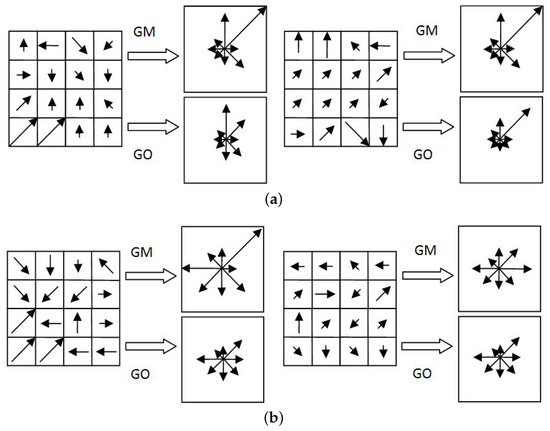
Figure 1.
Illustration of the difference between Gradient Magnitude (GM)-based descriptors and Gradient Occurrence (GO)-based descriptors. (a) Same GM-based descriptors and different GO-based descriptors are built for different image local regions. (b) Same GO-based descriptors and different GM-based descriptors are built for different image local regions.
Figure 2 shows a strategy of combining GM and GO has been proposed in [8] by intersecting the keypoint matches which are obtained by matching GM-based and GO-based descriptors individually. Unlike the aforementioned combination strategy [8], this paper presents four novel strategies of weighting GO and GM to generate new descriptors. The difference between the combination strategy [8] and the proposed weighting strategies is clearly illustrated in Figure 2. The proposed strategies of weighting GM and GO are summarized as follows.
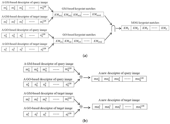
Figure 2.
Illustration of the difference between the combination strategy in [8] and the proposed weighting strategies of this paper. (a) The strategy of combining GM and GO proposed in [8] intersects the keypoint matches that are obtained by matching GM-based and GO-based descriptors individually. (b) The proposed strategies of this paper weight GM-based and GO-based descriptors, leading to new descriptors.
- (1)
- GM-based descriptors are normalized piecewise to reduce the side effect of substantial intensity variations between corresponding parts of multi-modal images. The normalizing operation is performed in two ways, i.e., descriptor normalization and histogram normalization (Strategies 1 and 2).
- (2)
- In the cases in which the values in GM-based descriptors are very small or not noticeable, the values at corresponding dimensions in GO-based descriptors are suppressed, thereby better distinguishing substantial intensity variations between corresponding parts of multi-modal images (Strategy 3).
- (3)
- A GM-based descriptor is incremented onto a GO-based descriptor to build a new descriptor which contains two types of gradient information simultaneously (Strategy 4).
These four strategies will be evaluated against GM and GO as well as their combination strategy in registering various types of multi-modal images.
The rest of this paper is organized as follows. Section 2 summarizes SIFT-based local descriptors, and the utilization of gradient information. In Section 3, the proposed strategies of weighting GM and GO are presented in detail, followed by a performance study in Section 4. Section 5 concludes this paper.
2. Related Work
This section will summarize SIFT-like local image descriptors and two types of gradient information, i.e., GM and GO. Furthermore, Magnitude and Occurrence of Gradient (MOG) [8] which combines GM and GO will be introduced briefly.
2.1. SIFT Based Local Image Descriptors
In the domain of mono-modal image registration, SIFT shows great effectiveness so that it has been widely studied and improved such as [11,20,33,34,35]. However, it has been pointed out in [22] that gradient orientations of corresponding feature points across multi-modal images may point to opposite directions. This phenomenon is called gradient reversal [8,11,26,36]. Hence, when SIFT descriptors are employed to deal with multi-modal images, the performance is usually undesirable. To address this issue, Symmetric SIFT (S-SIFT) [22] was proposed. The main steps of S-SIFT are as follows. First, the range of gradient orientations is restricted to [, ) once the gradient magnitudes and orientations are computed for all pixels within the neighborhood of a keypoint. Second, gradient magnitudes and orientations are computed for each local region that is rotated by relative to the original local region. Third, a S-SIFT descriptor is generated by combining two intermediate descriptors that are built for the original region and the rotated region. The S-SIFT descriptor achieves invariance to gradient reversal. However, the process of combining two intermediate descriptors causes ambiguities and sacrifices the discriminative power of descriptors [26,36]. Consequently, the same S-SIFT descriptor may be built for two local regions in which their image contents are actually largely different.
To address this issue, S-SIFT was improved in Improved Symmetric SIFT (IS-SIFT) [26,36] and its major steps are summarized as follows. First, S-SIFT is performed on two images to obtain a set of tentative keypoint matches. Second, the rotation difference between these two images is estimated by averaging the main orientation differences that underlie the tentative keypoint matches. Third, the estimated rotation difference is used to rotate the target image. Lastly, keypoint descriptors are re-built in two images as done in building a S-SIFT intermediate descriptor.
2.2. Gradient Magnitudes and Gradient Occurrences
Gradient magnitude of an image pixel is computed by
where
where denotes the intensity of the image pixel at location in the Gaussian smoothed image. In SIFT, the local region around a keypoint is divided into sub-regions and each sub-region is represented by an 8-bin orientation histogram. With Equation (1), the GM values are incremented at each bin of orientation histograms. When building an orientation histogram for the sub-region where there exist m pixels, is used to denote the qth orientation bin of this histogram. Thus, the GM value of the orientation bin can be computed by
where is the GM of the ith pixel of the qth bin in the (x,y) sub-region.
Based on the analysis in [26], GM potentially brings ambiguity that the same orientation histogram may be built for visually largely different regions. Therefore, GO was proposed in [26,32] as a new type of gradient information to build SIFT-like descriptor. When using GO to build an orientation histogram for a region, each bin of the histogram represents the number of occurrences of image gradients in corresponding orientation. In other words, if an image gradient occurs, the corresponding orientation bin will be incremented by 1. According to the definition in [26,32], GO can be computed by
where denotes the GM values of n pixels at a specific bin of an orientation histogram, that is, there exist n occurrences of image gradients at this orientation bin. When using GO for building descriptors, the value for this orientation bin is n, which is independent of specific GM values of these n pixels.
As pointed out in [8], utilizing GO to build orientation histograms brings ambiguity as well, that is, the same orientation histogram may be built for two regions with totally different image contents if the numbers of GOs of these two regions are equivalent. Therefore, both GM and GO are important gradient information for building local image descriptors. However, neither GM nor GO is sufficiently discriminative to perform well in all circumstances.
2.3. Magnitude and Occurrence of Gradient
In [8], MOG was proposed by combining GM and GO in building and matching SIFT-like descriptors. The main idea of MOG is summarized as follows. First, both GM-based and GO-based descriptors are built for each keypoint that has been detected in two images. Second, GM-based and GO-based descriptors are matched individually to obtain keypoint matches, respectively. Third, GM-based and GO-based keypoint matches are intersected to constitute the final keypoint matches.
For the purpose of performance comparisons, IS-SIFT will be used as the GM-based descriptor. When GO and MOG are incorporated into IS-SIFT, the merged feature description techniques are called GO-IS-SIFT and MOG-IS-SIFT, respectively.
3. Proposed Strategies of Weighting GM and GO
This section elaborates the proposed strategies of weighting GM and GO for building new SIFT-like descriptors. Strategies 1 and 2 aim at reducing the influence of substantial intensity variations between multi-modal images. To this end, GM-based descriptors are normalized piecewise. Strategy 1 normalizes the entire descriptor, whereas each orientation histogram is normalized in Strategy 2. Strategy 3 suppresses small gradient magnitudes when building GO-based descriptors. Strategy 4 increments a GM-based descriptor onto a GO-based descriptor to generate a new descriptor.
3.1. Normalizing GM-Based Descriptors (Strategies 1 and 2)
It is common that there exist substantial intensity variations between corresponding parts of multi-modal images [7,23,37]. As stated in Section 1 and Section 2.2, a SIFT-like descriptor is represented by a 128-dimensional vector and the value at each dimension is a GM value accumulated at a specific bin of an orientation histogram. In this manner, it is likely that largely different descriptors are built for corresponding parts of multi-modal images. To decrease the influence of substantial intensity variations between corresponding parts of multi-modal images, we propose to normalize GM-based SIFT-like descriptors.
Strategy 1: Normalizing an entire GM-based descriptor by four levels is performed as follows. First, all GM values of the descriptor are ranked by descending order. Second, these ranked GM values are divided into four ranking zones, i.e., (75%, 100%], (50%, 75%], (25%, 50%] and [0, 25%], respectively. These four ranking zones and their corresponding normalized GM values are listed in Table 1. Third, the value at each dimension is set to the corresponding normalized GM according to the ranking zone the original GM value should be assigned to. Similar to Table 1, GM-based descriptors can be normalized by 8 and 16 levels.

Table 1.
Normalizing Gradient Magnitude (GM) values by four levels.
Strategy 2: A similar strategy is proposed by normalizing each orientation histogram instead of normalizing the entire descriptor. As stated in Section 2.2, a SIFT-like descriptor consists of 16 orientation histograms and each histogram is built within a region around the keypoint. Unlike the aforementioned strategy which normalizes GM values in the domain of the entire local region around a keypoint, the normalization of GM values is performed in the domain of each sub-region in this strategy. As an orientation histogram only contains eight bins, Strategy 2 only does normalization by four levels. The normalized GM values are the same as Table 1 presents. The following consideration inspires us to narrow the normalization domain from the entire descriptor to each orientation histogram. When normalizing GM values of all dimensions of a descriptor, those dimensions which correspond to a sub-region will be set to the same normalized value if these dimensions are assigned to the same GM ranking zone. This phenomenon potentially affects the discriminative power of normalized descriptors. In such cases, performing GM normalization by each orientation histogram would be a better choice as compared to doing normalization by the entire descriptor.
There are two reasons for normalizing GM-based descriptors as follows. On the one hand, the more similar two descriptors are, the more likely these two descriptors are matched. Despite the fact that there is a normalization operation in building SIFT-like descriptors in order to diminish the influence of illumination, it has been found that there may exist a large difference in gradient magnitudes between descriptors of corresponding keypoints. On the other hand, the main orientation of a keypoint is decided by a set of gradient orientations within the local region surrounding the keypoint. If the image is influenced by illumination and noise seriously, main orientations of keypoints are likely to be incorrect. By normalizing GM values, the side effect caused by substantial intensity variations will potentially be weakened. Nevertheless, it should be noted that normalizing gradient magnitudes piecewise too much or too little will go to extremes and decrease the effectiveness of the proposed strategy.
3.2. Suppressing GO-Based Descriptors (Strategy 3)
Both GM-based and GO-based descriptors have limitations when building SIFT-like descriptors. GO-based descriptors better distinguish substantial intensity variations between corresponding parts of images as compared to GM, however, detailed image information is not captured by GO-based descriptors. As analyzed in [8], GO based-descriptors may be exactly the same for two regions whose image contents are totally different.
A small GM value implies the intensity change around the pixel is small, indicating that the gradient occurrence is not that noticeable. From this perspective, we propose that when the value in GM-based descriptors is very small, the value at the corresponding dimension in GO-based descriptor is set to zero. By doing so, the GO-based descriptors are likely to be more discriminative in distinguishing substantial intensity variations between images.
The main steps of this strategy are as follows. First, all values in a GM-based descriptor are ranked in descending order. Second, those 16 smallest values of the GM-based descriptor are labeled. Third, the corresponding dimensions of these 16 smallest GM values are found in the GO-based descriptor. Lastly, those labeled dimensions in the GO-based descriptor are set to zero. These four steps are illustrated in Figure 3.
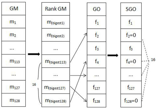
Figure 3.
The main steps of suppressing small gradient magnitudes in a GO-based descriptor (Strategy 3). From left to right, (1): Ranking a GM-based descriptor; (2): Labeling those dimensions which hold 16 smallest values; (3): Finding the corresponding dimensions in the GO-based descriptor; (4): Resetting the values of those labeled dimensions in the GO-based descriptor to zero.
Mathematically, this strategy is expressed as
In the experiments, the following thresholds are tested, including 1/16, 1/8 and 1/4 smallest values of the GM-based descriptor. Empirically, the 1/4 threshold achieves the best performance.
3.3. Incrementing GM-Based Descriptor onto GO-Based Descriptor (Strategy 4)
Unlike the MOG [8], Strategy 4 increments a GM-based descriptor onto the corresponding GO-based descriptor to generate a new descriptor. This strategy puts emphasis on the feature description stage, whereas MOG focuses on refining the keypoint matches. The motivation of this strategy is to verify the effectiveness of building descriptors by utilizing GM and GO in a straightforward way. The merged descriptor is more informative, which can be expressed as
where and denote the GM-based and GO-based descriptors, respectively. More intuitively, the new descriptor can be expressed as
where — denote the GM-based descriptor, — denote the GO descriptor built for the same keypoint.
For the referencing purpose, the following abbreviations are used to denote each of the aforementioned weighting strategies of GM and GO.
- 1.
- NGMD: Normalizing a GM-based descriptor by the entire descriptor (Strategy 1);
- 2.
- NGMH: Normalizing a GM-based descriptor by each orientation histogram (Strategy 2);
- 3.
- SGO: Suppressing a GO-based descriptor by ignoring the corresponding dimensions of small values in the GM-based descriptor (Strategy 3);
- 4.
- IMOG: Incrementing a GM-based descriptor onto a GO-based descriptor (Strategy 4).
4. Performance Study
For the purpose of performance comparisons, IS-SIFT and GO-IS-SIFT [8] are used for building the GM-based and GO-based descriptors, respectively. The proposed strategies of weighting GM and GO, i.e., NGMD, NGMH, SGO and IMOG, are evaluated against GM, GO and MOG [8] in registering multi-modal images.
4.1. Evaluation Metrics
The accuracy of an image registration technique depends highly on the matching accuracy. The higher the matching accuracy is, the more accurate the final registration will be [8]. Thus, the proposed strategies of weighting GM and GO are evaluated by
Moreover, recall vs 1-precision [20,38,39] is used for performance comparisons. The recall vs 1-precision is defined as
where is the ground-truth number of matches. The in Equation (10) is simply the equivalent of defined in Equation (8). The recall vs 1-precision curve is generally plotted for a particular image pair [6,20]. To make statistics on a set of image pairs, the area under the recall vs 1-precision curve [38] will be used.
The ground-truths of test image pairs are all known or provided. A maximum of four pixels error is considered when deciding whether a match is correct or not, which is consistent with existing literature [5,8,40].
4.2. Test Datasets
The following five datasets are tested. The first dataset consists of 18 NIR (Near Infra-Red) vs EO (Electro-Optical) image pairs from several sources [20,21,41,42] (Dataset 1). The second and third datasets are transverse and coronal T1 vs T2 weighted MRI brain images respectively (Datasets 2 and 3). These two datasets were collected from McConnell Brain Imaging Center (McConnell Brain Imaging Center: https://www.mcgill.ca/bic/home). There are 87 and 101 image pairs in Datasets 2 and 3 respectively. The fourth dataset consists of 32 pairs of satellite images from different bands and can be downloaded on this website (https://serc.carleton.edu/index.html). The fifth dataset is SYM dataset that consists of 46 image pairs involving different depictions (drawing vs. photo), different time periods (modern vs. historical), and different illuminations (day vs. night) [43] (Dataset 5). In total, 284 image pairs are tested. Sample image pairs of these five datasets are shown in Figure 4.
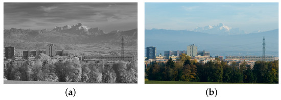
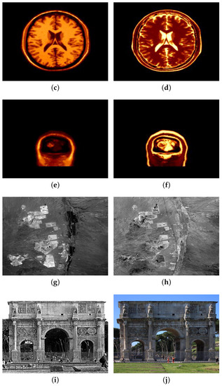
Figure 4.
Sample image pairs of Datasets 1 to 5. (a,b) NIR vs EO (Dataset 1). (c,d) transverse T1 vs T2 MRI (Dataset 2). (e,f) coronal T1 vs T2 MRI (Dataset 3). (g,h) satellite images from different bands (Dataset 4). (i,j) SYM dataset (Dataset 5).
4.3. Experimental Results
For a clear comparison, the average accuracy achieved by each compared technique for each dataset is listed in Table 2. Overall, the following trends can be derived from Table 2. First, GO-based descriptors generally achieve higher accuracy as compared to GM-based descriptor, which has also been reported in [8,36]. Second, the proposed NGMD (16 levels) achieves an overall matching accuracy that is close to what MOG obtains. These two techniques outperform the others in terms of matching accuracy. However, it is noted that MOG only refines the matching result and does not generate new descriptors, as stated in Section 2.3. In contrast, each of the proposed strategies builds new SIFT-like descriptors by appropriately weighting GM and GO. Third, each of the proposed strategies achieves higher accuracy as compared to both GM and GO. This indicates that these three proposed strategies are more robust to gradient changes between multi-modal images and have higher discriminative power as compared to GM and GO.
Table 2.
Comparisons in average accuracy between the compared techniques on each dataset. The horizontal line below MOG separates three existing techniques and the proposed strategies of weighting GM and GO. The accuracy in the last column is obtained by doing the average on all five datasets.
Figure 5 shows an example of matching results when registering the sample image pair shown in Figure 4e,f. Among these compared techniques, NGMH comes first with a 100% accuracy. The proposed NGMD(4 levels), NGMD(8 levels), NGMD(16 levels), NGMH and SGO achieve higher accuracy as compared to the existing GM, GO and MOG. The proposed IMOG outperforms both GM and GO, but performs slightly worse as compared to MOG.
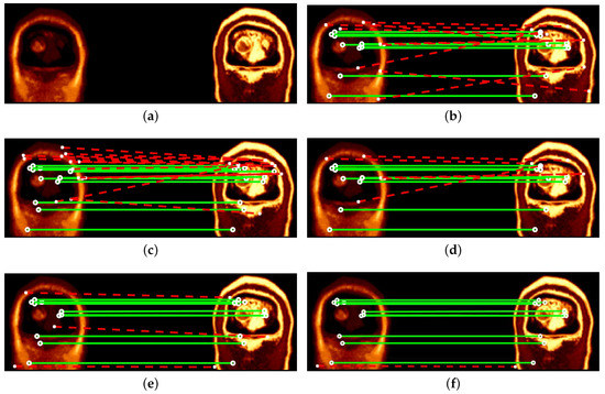
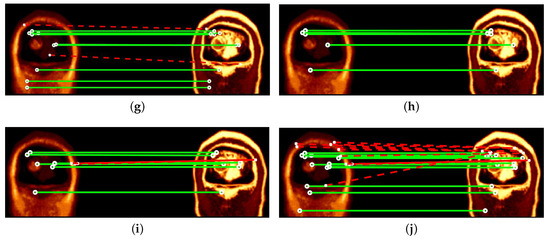
Figure 5.
Comparisons in matching results for a pair of coronal T1 vs T2 weighted MRI brain images from Dataset 3. Green (solid) and red (dashed) lines indicate correct and incorrect matches respectively. (a) Original image pair. (b) GM: 9/18 = 50.00%. (c) GO: 12/26 = 46.15%. (d) MOG: 8/13 = 61.54%. (e) NGMD(4 levels): 11/14 = 78.57%. (f) NGMD(8 levels): 11/12 = 91.67%. (g) NGMD(16 levels): 9/11 = 81.82%. (h) NGMH: 5/5 = 100%. (i) SGO: 7/9 = 77.78%. (j) IMOG: 13/24 = 54.17%.
Moreover, Figure 6 compares the recall results of the seven compared techniques on Datasets 1 to 5. Figure 6b only shows the recall results of 18 image pairs that have been randomly sampled from Datasets 2 and 3. Similarly, Figure 6c,d show the recall results of 16 and 23 image pairs that have been sampled from Datasets 4 and 5, respectively. Apart from these sample image pairs, the recall results of the remaining pairs show a similar trend as Figure 6b–d, which is because all image pairs of the same dataset have similar characteristics. Showing a part of recall results in Figure 6b–d is to make a better illustration between the compared techniques. In order to clearly compare the recall results of the compared methods, Figure 7 plots the recall vs precision curves of five image pairs that have been randomly selected from each dataset. Table 3 compares the area under the recall vs 1-precision curve achieved by the seven compared techniques. By analyzing the results presented in Figure 6 and Figure 7 and Table 3, the following trends can be drawn.
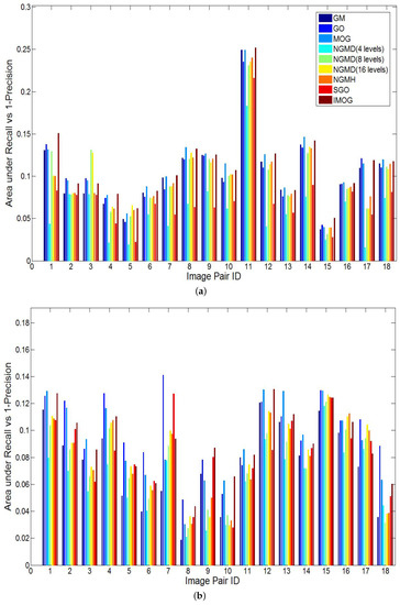
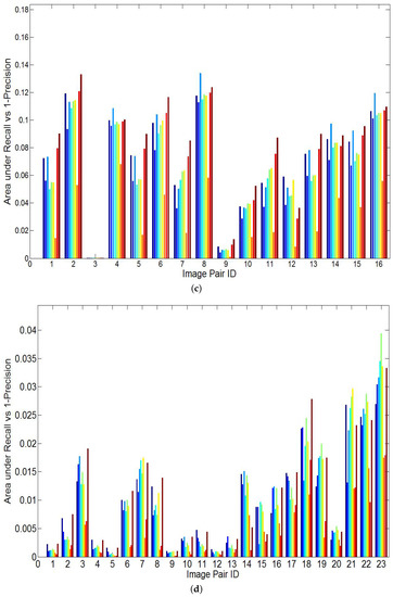
Figure 6.
Comparisons in the area under the recall vs 1-precision curve. (a) NIR vs EO (Dataset 1). (b) Sample pairs of transverse and coronal T1 vs T2 MRI (Datasets 2 and 3). (c) Sample pairs of satellite images from different bands (Dataset 4). (d) Sample pairs of SYM dataset (Dataset 5).
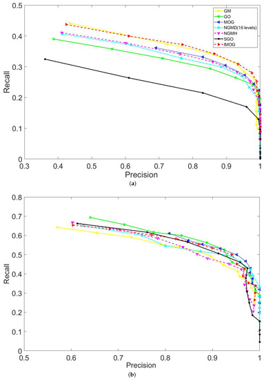
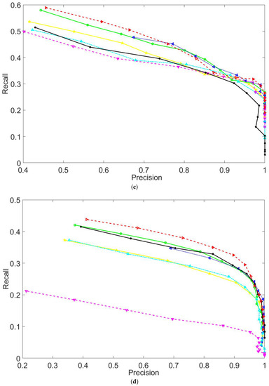
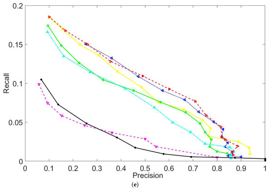
Figure 7.
Comparisons in the recall vs precision curves. (a–e) show the recall vs precision curves for sample image pairs that are randomly selected from Datasets 1 to 5, respectively.
Table 3.
Comparisons in the area under the recall vs 1-precision curve for Datasets 1 to 5. Randomly sampled image pairs of Datasets 1 to 5 are tested. Higher results are better.
Overall, the proposed IMOG achieves the best recall results among all compared techniques. The proposed NGMH achieves the lowest recall results. This strategy of weighting GM and GO actually obtains a high matching accuracy by preserving a small set of keypoint matches, which can be seen from the example of matching results shown in Figure 5.
4.4. Efficiency Comparison
The experiments were implemented in Matlab R2014b on a Windows 7 PC with Intel i7 CPU of 3.4 GHz and 8 GB memory. Figure 8 compares the runtime of all seven compared techniques when registering coronal T1 vs T2 weighted MRI brain images (Dataset 3). Note that the runtime for the four Datasets show a similar trend as Figure 8. For all five datasets, the average runtime for GM, GO, MOG, NGMD(4 levels), NGMD(8 levels), NGMD(16 levels), NGMH, SGO, IMGO are 7.30, 7.43, 15.70, 7.53, 7.38, 7.36, 7.23, 8.08 and 11.24 seconds, respectively. Obviously, MOG is the most time-consuming one among all compared techniques as it needs to build and match GM-based and GO-based descriptors individually.
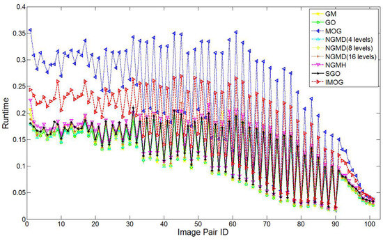
Figure 8.
Efficiency comparison on Dataset 3.
4.5. Discussions
Despite the fact that it has been found that GM and GO are complementary gradient information [8], to the best of our knowledge, there exists no literature which builds new SIFT-like descriptors by taking into account both GM and GO. This paper aims to address this issue. In the cases there exist substantial gradient changes between corresponding parts of the multi-modal image, GM-based local descriptors usually perform poorly in registering this kind of images. It has been pointed out that GO also has limitations in building local descriptors [8]. Both GM and GO are important and these two types of gradient information are complementary [8]. Based on this analysis, a strategy of combining GM and GO has been proposed in [8], which is achieved by intersecting the keypoint matches which are obtained by matching GM-based and GO-based descriptors individually. In this paper, four novel strategies of weighting GM and GO are proposed to build new SIFT-like descriptors, thereby achieving greater robustness to gradient changes across multi-modal images.
Experimental results can be briefly summarized as follows.
- (1)
- From the perspective of building new descriptors, each of the proposed strategies of weighting GM and GO achieves higher accuracy as compared to both GM and GO. Overall, the proposed NGMD that normalizes GM-based descriptors by 16 levels achieves the highest matching accuracy, while excluding MOG. It should be noted that each of the proposed strategies of weighting GM and GO creates new SIFT-like descriptors, whereas MOG only intersects the keypoint matches obtained by GM-based and GO-based descriptors.
- (2)
- In terms of recall performance, the proposed IMOG achieves the best recall results, whereas the proposed NGMH obtains the lowest recall performance among the seven compared techniques.
- (3)
- With regards to efficiency, MOG is the least efficient one as it builds and matches GM-based and GO-based descriptors individually, and then intersects two sets of keypoint matches. Compared with MOG, the proposed IMOG is more efficient in that it only increments GM-based descriptors onto GO-based descriptors, thereby doubling the dimensionality of descriptors. The other compared techniques take comparable runtime, and are far more efficient as compared to MOG and IMOG.
5. Conclusions
This paper explores the utilization of two types of gradient information, i.e., GM and GO. Four novel strategies of weighting GM and GO have been presented and extensively evaluated using five image registration datasets. The experimental results have shown the effectiveness of the proposed techniques. From the perspective of building new descriptors, the proposed NGMD (16 levels) is recommended as the best choice for multi-modal image registration, when taking into account both matching accuracy and recall.
On the basis of GM-based and GO-based descriptors, the proposed weighting strategies lead to novel local descriptors. Without loss of generality, these novel local descriptors are applicable to those research problems that demand local image representation.
Author Contributions
G.D. and H.Y. performed the experiments, wrote and revised the manuscript; G.L. conceived the work, designed the experiments, guided and revised the manuscript; X.D. analyzed the experimental results. All authors read and approved the final manuscript.
Funding
This work was supported by the Natural Science Foundation of Shandong Province (Grant No. ZR2017LF005) and the National Natural Science Foundation of China (Grant No. 61802212, No. 61802213).
Conflicts of Interest
The authors declare no conflict of interest.
References
- Mikolajczyk, K.; Tuytelaars, T. Local image features. Encycl. Biom. 2009, 939–943. [Google Scholar] [CrossRef]
- Lowe, D.G. Distinctive image features from scale-invariant keypoints. Int. J. Comput. Vis. 2004, 60, 91–110. [Google Scholar] [CrossRef]
- Dubey, S.R.; Singh, S.K.; Singh, R.K. Local wavelet pattern: A new feature descriptor for image retrieval in medical CT databases. IEEE Trans. Image Process. 2015, 24, 5892–5903. [Google Scholar] [CrossRef] [PubMed]
- Lv, G. “ℓmp: A novel similarity measure for matching local image descriptors. IEEE Access 2018, 6, 55315–55325. [Google Scholar] [CrossRef]
- Lv, G. A novel correspondence selection technique for affine rigid image registration. IEEE Access 2018, 6, 32023–32034. [Google Scholar] [CrossRef]
- Lv, G.; Teng, S.W.; Lu, G. Enhancing image registration performance by incorporating distribution and spatial distance of local descriptors. Pattern Recognit. Lett. 2018, 103, 46–52. [Google Scholar] [CrossRef]
- Lv, G.; Teng, S.W.; Lu, G. COREG: A corner based registration technique for multimodal images. Multimed. Tools Appl. 2018, 77, 12607–12634. [Google Scholar] [CrossRef]
- Lv, G.; Teng, S.W.; Lu, G. Enhancing SIFT-based image registration performance by building and selecting highly discriminating descriptors. Pattern Recognit. Lett. 2016, 84, 156–162. [Google Scholar] [CrossRef]
- Zitova, B.; Flusser, J. Image registration methods: A survey. Image Vis. Comput. 2003, 21, 977–1000. [Google Scholar] [CrossRef]
- Oliveira, F.P.; Tavares, J.M.R. Medical image registration: A review. Comput. Methods Biomech. Biomed. Eng. 2014, 17, 73–93. [Google Scholar] [CrossRef]
- Lv, G. Self-Similarity and symmetry with SIFT for multi-modal image registration. IEEE Access 2019, 7, 52202–52213. [Google Scholar] [CrossRef]
- Ma, J.; Jiang, J.; Zhou, H.; Zhao, J.; Guo, X. Guided locality preserving feature matching for remote sensing image registration. IEEE Trans. Geosci. Remote Sens. 2018, 56, 4435–4447. [Google Scholar] [CrossRef]
- Fu, Z.; Qin, Q.; Luo, B.; Sun, H.; Wu, C. HOMPC: A local feature descriptor based on the combination of magnitude and phase congruency information for multi-sensor remote sensing images. Remote Sens. 2018, 10, 1234. [Google Scholar] [CrossRef]
- Lv, G. Robust and Effective Techniques for Multi-Modal Image Registration. Ph.D. Thesis, Monash University, Melbourne, VIC, Australia, 2015. [Google Scholar]
- Yang, K.; Pan, A.; Yang, Y.; Zhang, S.; Ong, S.; Tang, H. Remote sensing image registration using multiple image features. Remote Sens. 2017, 9, 581. [Google Scholar] [CrossRef]
- Hossain, M.T. An Effective Technique for Multi-Modal Image Registration. Ph.D. Thesis, Monash University, Melbourne, VIC, Australia, 2012. [Google Scholar]
- Han, X.H.; Chen, Y.W.; Xu, G. High-order statistics of weber local descriptors for image representation. IEEE Trans. Cybern. 2015, 45, 1180–1193. [Google Scholar] [CrossRef] [PubMed]
- Mandal, B.; Wang, Z.; Li, L.; Kassim, A.A. Performance evaluation of local descriptors and distance measures on benchmarks and first-person-view videos for face identification. Neurocomputing 2016, 184, 107–116. [Google Scholar] [CrossRef]
- Turan, C.; Lam, K.M. Histogram-based local descriptors for facial expression recognition (FER): A comprehensive study. J. Vis. Commun. Image Represent. 2018, 55, 331–341. [Google Scholar] [CrossRef]
- Mikolajczyk, K.; Schmid, C. A performance evaluation of local descriptors. IEEE Trans. Pattern Anal. Mach. Intell. 2005, 27, 1615–1630. [Google Scholar] [CrossRef]
- Kelman, A.; Sofka, M.; Stewart, C.V. Keypoints descriptors for matching across multiple image modalities and non-linear intensity variations. In Proceedings of the 2007 IEEE Conference on Computer Vision and Pattern Recognition, Minneapolis, MN, USA, 17–22 June 2007; pp. 1–7. [Google Scholar]
- Chen, J.; Tian, J. Real-time multi-modal rigid registration based on a novel symmetric-SIFT descriptor. Prog. Nat. Sci. 2009, 19, 643–651. [Google Scholar] [CrossRef]
- Chen, J.; Tian, J.; Lee, N.; Zheng, J.; Smith, R.T.; Laine, A.F. A partial intensity invariant feature descriptor for multimodal retinal image registration. IEEE Trans. Biomed. Eng. 2010, 57, 1707–1718. [Google Scholar] [CrossRef]
- Ghassabi, Z.; Shanbehzadeh, J.; Sedaghat, A.; Fatemizadeh, E. An efficient approach for robust multimodal retinal image registration based on UR-SIFT features and PIIFD descriptors. EURASIP J. Image Video Process. 2013, 1, 1–16. [Google Scholar] [CrossRef]
- Saleem, S.; Sablatnig, R. A robust SIFT descriptor for multispectral images. IEEE Signal Process. Lett. 2014, 21, 400–403. [Google Scholar] [CrossRef]
- Teng, S.W.; Hossain, M.T.; Lu, G. Multimodal image registration technique based on improved local feature descriptors. J. Electron. Imaging 2015, 24, 013013-1–013013-17. [Google Scholar] [CrossRef]
- Zhang, S.; Tian, Q.; Lu, K.; Huang, Q.; Gao, W. Edge-SIFT: Discriminative binary descriptor for scalable partial-duplicate mobile search. IEEE Trans. Image Process. 2013, 22, 2889–2902. [Google Scholar] [CrossRef]
- Ma, W.; Wen, Z.; Wu, Y.; Jiao, L.; Gong, M.; Zheng, Y.; Liu, L. Remote sensing image registration with modified SIFT and enhanced feature matching. IEEE Geosci. Remote Sens. Lett. 2017, 14, 3–7. [Google Scholar] [CrossRef]
- Li, Y.; Stevenson, R.L. Incorporating global information in feature-based multimodal image registration. J. Electron. Imaging 2014, 23, 023013. [Google Scholar] [CrossRef]
- Heinrich, M.P.; Jenkinson, M.; Bhushan, M.; Matin, T.; Gleeson, F.V.; Brady, M.; Schnabel, J.A. MIND: Modality independent neighbourhood descriptor for multi-modal deformable registration. Med. Image Anal. 2012, 16, 1423–1435. [Google Scholar] [CrossRef]
- Addison Lee, J.; Cheng, J.; Hai Lee, B.; Ping Ong, E.; Xu, G.; Wing Kee Wong, D.; Liu, J.; Laude, A.; Han Lim, T. A low-dimensional step pattern analysis algorithm with application to multimodal retinal image registration. In Proceedings of the 28th IEEE Conference on Computer Vision and Pattern Recognition, Boston, MA, USA, 7–12 June 2015; pp. 1046–1053. [Google Scholar]
- Hossain, M.T.; Teng, S.W.; Lu, G.; Lackmann, M. An enhancement to SIFT-Based techniques for image registration. In Proceedings of the 2010 International Conference on Digital Image Computing: Techniques and Applications, Sydney, NSW, Australia, 1–3 December 2010; pp. 166–171. [Google Scholar]
- Bay, H.; Ess, A.; Tuytelaars, T.; Van Gool, L. Speeded-up robust features (SURF). Comput. Vis. Image Underst. 2008, 110, 346–359. [Google Scholar] [CrossRef]
- Morel, J.M.; Yu, G. ASIFT: A new framework for fully affine invariant image comparison. SIAM J. Imaging Sci. 2009, 2, 438–469. [Google Scholar] [CrossRef]
- Liu, C.; Yuen, J.; Torralba, A. SIFT Flow: Dense correspondence across scenes and its applications. IEEE Trans. Pattern Anal. Mach. Intell. 2011, 33, 978–994. [Google Scholar] [CrossRef]
- Hossain, M.T.; Lv, G.; Teng, S.W.; Lu, G.; Lackmann, M. Improved symmetric-SIFT for multi-modal image registration. In Proceedings of the 2011 International Conference on Digital Image Computing: Techniques and Applications, Noosa, QLD, Australia, 6–8 December 2011; pp. 197–202. [Google Scholar]
- Wachinger, C.; Navab, N. Entropy and laplacian images: Structural representations for multi-modal registration. Med. Image Anal. 2012, 16, 1–17. [Google Scholar] [CrossRef]
- Levi, G.; Hassner, T. LATCH: Learned arrangements of three patch codes. In Proceedings of the 2016 IEEE Winter Conference on Applications of Computer Vision (WACV), Lake Placid, NY, USA, 7–10 March 2016; pp. 1–9. [Google Scholar]
- Fan, J.; Wu, Y.; Wang, F.; Zhang, P.; Li, M. New point matching algorithm using sparse representation of image patch feature for SAR image registration. IEEE Trans. Geosci. Remote Sens. 2017, 55, 1498–1510. [Google Scholar] [CrossRef]
- Yang, G.; Stewart, C.V.; Sofka, M.; Tsai, C.L. Registration of challenging image pairs: Initialization, estimation, and decision. IEEE Trans. Pattern Anal. Machine Intell. 2007, 29, 1973–1989. [Google Scholar] [CrossRef]
- Kim, Y.S.; Lee, J.H.; Ra, J.B. Multi-sensor image registration based on intensity and edge orientation information. Pattern Recognit. 2008, 41, 3356–3365. [Google Scholar] [CrossRef]
- Fredembach, C.; Susstrunk, S. Illuminant estimation and detection using near infrared. In Proceedings of the Digital Photography V, IS&T-SPIE Electronic Imaging Symposium, San Jose, CA, USA, 19 January 2009; p. 72500E. [Google Scholar]
- Hauagge, D.C.; Snavely, N. Image matching using local symmetry features. In Proceedings of the 2012 IEEE Conference on Computer Vision and Pattern Recognition, Providence, RI, USA, 16–21 June 2012; pp. 206–213. [Google Scholar]
© 2019 by the authors. Licensee MDPI, Basel, Switzerland. This article is an open access article distributed under the terms and conditions of the Creative Commons Attribution (CC BY) license (http://creativecommons.org/licenses/by/4.0/).