A Novel Noise Suppression Channel Estimation Method Based on Adaptive Weighted Averaging for OFDM Systems

Abstract

Orthogonal frequency division multiplexing (OFDM) systems have inherent symmetric properties, such as coding and decoding, constellation mapping and demapping, inverse fast Fourier transform (IFFT) and fast Fourier transform (FFT) operations corresponding to multi-carrier modulation and demodulation, and channel estimation is a necessary module to resist channel fading in the OFDM system. However, the noise in the channel will significantly affect the accuracy of channel estimation, which further affects the recovery quality of the final received signals. Therefore, this paper proposes an efficient noise suppression channel estimation method for OFDM systems based on adaptive weighted averaging. The basic idea of the proposed method is averaging the last few channel coefficients obtained from coarse estimation to suppress the noise effect, while the average frame number is adaptively adjusted by combining Doppler spread and signal-to-noise ratio (SNR) information. Meanwhile, to better combat the negative effect brought by Doppler spread and inter-carrier interference (ICI), the proposed method introduces a weighting factor to correct the weighted value of each frame in the averaging process. Simulation results show that the proposed channel estimation method is effective and provides better performance compared with other conventional channel estimation methods.

1. Introduction

Orthogonal frequency division multiplexing (OFDM) technology is widely used in modern communication systems for its superior performance and high spectral efficiency [1,2]. The cyclic prefix (CP) is inserted between the adjacent OFDM symbols as a guard interval (GI), which not only reduces the inter-symbol interference (ISI) largely, but also simplifies the design of the frequency-domain equalizer [3]. For these reasons, OFDM technology has been applied to many transmission standards such as digital video broadcasting-terrestrial (DVB-T) and wireless local area network (WLAN) [4]. In recent years, the applications of the OFDM system in underwater acoustic communication, smart grid, vehicular ad-hoc network and other fields have also received extensive attention and research [5,6,7]. The transmission reliability of OFDM systems can be further enhanced by using the multiple-input multiple-output (MIMO) technique without increasing the bandwidth [8,9]. Offset quadrature amplitude modulation (OQAM) can also be combined with OFDM to make the system have lower spectral sidelobes by using the pulse shaping filters, which is a candidate technology for 5G communication [10,11]. In OFDM systems, channel estimation is an important module for coherent detection and frequency-domain equalization, and the accuracy of channel estimation directly affects the recovery quality of the final received OFDM signals [12,13]. However, channel estimation is a challenging technology in wireless systems due to the noise effect and time variance of wireless channels [14,15].

There have been many researches on channel estimation in OFDM systems. In general, channel estimation methods can be divided into three categories: pilot-based channel estimation, blind channel estimation, and semi-blind channel estimation [16]. Blind and semi-blind estimation perform channel estimation with non-pilot and few pilots, respectively, and thus have higher spectral efficiency. However, these two methods suffer from high computational complexity and are not preferred in practice. Due to reliability and simplicity, the pilot-based channel estimation is more attractive in practical applications [12]. Pilot-based channel estimation method estimates the channel impulse response (CIR) or channel frequency response (CFR) by multiplexing the known pilot sequences into OFDM symbols. In practice, pilot symbols are inserted in various patterns, such as block-type, comb-type, and scatter-type, to adapt to different channel environments [16]. In this paper, comb-type pilot-based channel estimation is used in OFDM systems since comb-type pilot is more robust to a time-varying channel with low to high Doppler spread.

To suppress the noise effect in the channel and obtain more accurate channel estimation results, this paper proposes an adaptive weighted averaging (AWA)-based noise suppression channel estimation method. The essence of the proposed method is to average the last few channel coefficients obtained from coarse estimation to suppress the noise effect, while the average frame number is adaptively adjusted by combining Doppler spread and signal-to-noise ratio (SNR) information. Moreover, to better combat the negative effect of the Doppler spread and inter-carrier interference (ICI), this paper introduces a weighting factor to correct the weighted value of each frame in the averaging process. Simulation results show that the proposed method outperforms the conventional counterparts in terms of bit error rate (BER) and normalized mean square error (NMSE).

The remainder of this paper is organized as follows. Section 2 illustrates the related work and the system model is presented in Section 3. Section 4 introduces three conventional channel estimation methods. Section 5 details the proposed AWA-based noise suppression channel estimation method. The experimental results of the proposed method are presented in Section 6. Conclusions are presented in Section 7.

2. Related Work

There have been many conventional pilot-based channel estimation methods for OFDM systems, such as the least squares (LS) method [17], minimum mean square error (MMSE) method [18], and linear MMSE (LMMSE) method [19,20]. The LS method is the simplest channel estimation method and has been widely used for many years. However, the LS method ignores the noise effect, which greatly reduces its performance [17]. The MMSE method has good estimation performance by utilizing the channel statistic, but this method involves the inverse operation of the matrix, so its computational complexity is high [18]. To reduce the computational complexity of the MMSE method, the LMMSE method is implemented for channel estimation in the receiver of the OFDM system [19]. However, the LMMSE method requires a priori information to calculate the channel autocorrelation matrix and its implementation is somewhat difficult in fast fading channels.

In recent years, researchers have proposed some new channel estimation methods. Combining channel soft information and Turbo decoding in an iterative way can greatly improve the accuracy of channel estimation, which can be realized by the expectation maximization (EM) algorithm or belief propagation (BP) algorithm [21,22]. In [22], an iterative channel estimation based on a factor graph is proposed; this method iteratively passes soft information between the channel estimation and data decoding stages through the BP algorithm. The main disadvantage of this method is the high computational complexity caused by multiple iterations. Moreover, the EM algorithm is also widely used in fast fading channel estimation [21]. Based on the strong performance of deep learning, the deep learning-based channel estimation method is promising [23]. Different from existing OFDM receivers that first estimate channel state information (CSI) explicitly and then recover the transmitted symbols using the estimated CSI, the deep learning-based method estimates CSI implicitly and recovers the transmitted symbols directly, which has similar performance compared with the MMSE method and is more robust than conventional methods. However, the deep learning-based method requires massive amounts of training data samples, which is often difficult to obtain in practice [23].

The additive white Gaussian noise (AWGN) existing in wireless communication systems will significantly reduce the accuracy of channel estimation [24]. In recent years, researchers have put forward some noise suppression channel estimation methods. To suppress the noise effect, a threshold, which is often obtained through noise variance estimation, is applied at the LS estimation of the CIR to find the positions of the most significant taps (MSTs) [16,25]. However, a fixed threshold often cannot distinguish the paths with smaller energy from the noise. Linear filter in time domain is also an effective way to mitigate the noise effect, but it is not easy to determine the parameters of the linear filter in practical implementation [26]. In [27], an improved MMSE (IMMSE) channel estimation method is proposed. This method inherits the noise resistance of the MMSE method and simplifies the matrix calculation. However, this method suffers from a loss of the partial path energy while suppressing the noise, which decreases the estimation accuracy at high SNR scenarios. Moreover, for some wideband wireless channels, researchers have proved that the CIR often presents a sparse structure (i.e., the CIR indeed contain only a small proportion of nonzero valued coefficients) [28]. Such channels occur in radio [29] and underwater [30] communications. Some recent works exploit the channel sparsity to discard most of the noise effect in the zero-value taps, which can significantly improve the accuracy of the channel estimation [28,29,30].

Moreover, some researchers utilize the averaging of AWGN to further suppress the noise effect, which can be combined with the above-mentioned conventional noise suppression method [16,27,28,29,30]. In [31], a simple noise suppression channel estimation method based on inter-frame pilot averaging is proposed. This method can provide more accurate interpolation results because the noise power at the pilot position is suppressed by averaging adjacent frames. Meanwhile, a similar noise reduction method by averaging the channel coefficients of LS estimation in two or more OFDM frames is proposed in [32,33]. These averaging methods in [31,32,33], which use a fixed average frame number, can be implemented on time invariant channels and are very simple to implement in practice. However, it cannot be applied directly to dynamic channels, because the Doppler spread and the ensuing ICI in dynamic channels will bring Doppler distortion in the averaging process. With the increase of the Doppler spread, the estimation accuracy of the averaging method using a fixed average frame number deteriorates significantly. In [34,35], a more sophisticated adaptive averaging channel estimation method is proposed, which adjusts the average frame number according to the Doppler spread. However, the method in [34,35] does not further consider the relationship between the average frame number and SNR, so its performance is unstable under different SNR scenarios. On the other hand, a weighted inter-frame averaging method for coherent optical OFDM (CO-OFDM) system is proposed in [36], which uses a weighting factor between 0 and 1 to resist the phase rotation. Inspired by this method, this paper also introduces a weighting factor in the averaging process to resist the Doppler distortion.

To keep the performance of the averaging method optimal under different Doppler spread and SNR scenarios, this paper proposes an AWA-based noise suppression channel estimation method. As a unique feature of the averaging method, the proposed AWA method can be combined with other conventional noise suppression methods to further improve the noise suppression effect. In this paper, the proposed method is combined with the threshold value method [25] (i.e., taking threshold value estimation as the coarse estimation). This paper is novel in three points: First, it studies and analyzes the influence of Doppler spread and SNR on the averaging method and uses the combination of Doppler spread and SNR to adaptively determine the average frame number. Second, it introduces a weighting factor into the averaging process, which can improve the robustness against Doppler spread and ICI. Third, it combines the proposed method with the threshold value method to further suppress the noise in the MSTs.

In [37], researchers committed to determine the positions of the MSTs by counting the number of positive and negative CIR coefficients of multiple frames, which was consistent with the goal of the threshold value method. Therefore, the proposed method is different from the multi-frame statistical channel estimation method in [37]. Moreover, the proposed method can be further improved by combining the multi-frame statistical channel estimation method. To facilitate further research, channel model and some simulation parameters, the same as [37], are selected in this paper.

3. System Model

A CP-OFDM system [37] with $N$ subcarriers and utilizing the proposed channel estimation method, is presented in Figure 1, where $N_{\mathrm{P}}\le N$ uniformly spaced subcarriers are used as comb-type pilots. The pilots position arranged in ascending order is denoted as $P_1,P_2,\cdots ,P_{N_{\mathrm{P}}}$. This paper assumes that the system is perfectly synchronized and that the CP length $N_{\mathrm{G}}$ should be longer than the maximum channel delay spread $L$ (in terms of samples) to avoid the ISI problem. In the frequency selective channel, the pilot subcarriers spacing should not exceed the coherent bandwidth, which can be transformed to $N_{\mathrm{P}}\ge L$ [30]. Since $L$ is unknown, this paper chooses $N_{\mathrm{P}}\ge N_{\mathrm{G}}$ which guarantees that the above constraint is respected.

At the receiver, the fast Fourier transform (FFT) output of the pilot symbols is expressed as [22]:

$${\mathit{Y}}_{\mathrm{P}}={\mathit{X}}_{\mathrm{P}}{\mathit{F}}_{\mathrm{P}}\mathit{h}+\mathit{n},$$

(1)

where ${\mathit{Y}}_{\mathrm{P}}={[Y_1,Y_2,\cdots ,Y_{N_{\mathrm{P}}}]}^{\mathrm{T}}$ is the demodulated signal over the pilot subcarriers. ${\mathit{X}}_{\mathrm{P}}$ is a $N_{\mathrm{P}}\times N_{\mathrm{P}}$ diagonal matrix containing the pilot symbols and ${\mathit{F}}_{\mathrm{P}}$ is a $N_{\mathrm{P}}\times L$ Fourier submatrix indexed by $[P_1,P_2,\cdots ,P_{N_{\mathrm{P}}}]$ in row and $[1,2,\cdots ,L]$ in column, obtained from the standard $N\times N$ FFT matrix $\mathit{F}$ with entries ${\mathit{F}}_{l,m}={\mathrm{e}}^{-\mathrm{j}2\pi (l-1)(m-1)/N}$, where $l,m=1,2,\cdots ,N$. $\mathit{h}={[h_1,h_2,\cdots ,h_L]}^{\mathrm{T}}$ is the sampled equivalent CIR and $\mathit{n}={[n_1,n_2,\cdots ,n_{N_{\mathrm{P}}}]}^{\mathrm{T}}$ is the zero-mean complex AWGN with covariance matrix ${\sigma }^2{\mathit{I}}_{N_{\mathrm{P}}}$, i.e., $\mathit{n}~\mathcal{C}\mathcal{N}(0,{\sigma }^2{\mathit{I}}_{N_{\mathrm{P}}})$. After FFT transformation, the estimated CSI is obtained in the channel estimation block. The AWGN existing in the estimated channel coefficients is further suppressed in the adaptively weighted averaging block, which is detailed in Section 5.

4. Conventional Channel Estimation Methods

4.1. Time-Domain LS Channel Estimation

The LS method is the simplest channel estimation method for OFDM systems [17,38], and the CFR at the pilot subcarriers estimated by the LS method can be represented as:

$${\widehat{\mathit{H}}}_{\mathrm{P}}={\mathit{X}}_{\mathrm{P}}^{-1}{\mathit{Y}}_{\mathrm{P}}={\mathit{F}}_{\mathrm{P}}\mathit{h}+{\mathit{X}}_{\mathrm{P}}^{-1}\mathit{n}.$$

(2)

Ignoring the effects of the noise item ${\mathit{X}}_{\mathrm{P}}^{-1}\mathit{n}$, the CIR estimated by the LS method can be expressed as:

$${\widehat{\mathit{h}}}_{\mathrm{LS}}={\mathit{F}}_{\mathrm{P}}^{+}{\widehat{\mathit{H}}}_{\mathrm{P}}={\mathit{F}}_{\mathrm{P}}^{+}{\mathit{F}}_{\mathrm{P}}\mathit{h}+{\mathit{F}}_{\mathrm{P}}^{+}{\mathrm{X}}_{\mathrm{P}}^{-1}\mathit{n},$$

(3)

where ${\mathit{F}}_{\mathrm{P}}^{+}$ represents the pseudo-inverse matrix of ${\mathit{F}}_{\mathrm{P}}$, and ${\mathit{F}}_{\mathrm{P}}^{+}={({\mathit{F}}_{\mathrm{P}}^H{\mathit{F}}_{\mathrm{P}})}^{-1}{\mathit{F}}_{\mathrm{P}}^{\mathrm{H}}=(1/N_{\mathrm{P}}){\mathit{F}}_{\mathrm{P}}^H$. ${\mathit{F}}_{\mathrm{P}}^{\mathrm{H}}$ is the conjugate transposition of ${\mathit{F}}_{\mathrm{P}}$. Since $L$ is unknown, $N_{\mathrm{P}}$ replaces $L$ to guarantee that the estimated CIR length is longer than the actual CIR length. Thus, Equation (3) can be re-written as:

$${\widehat{\mathit{h}}}_{\mathrm{LS}}=\frac{1}{N_{\mathrm{P}}}{\mathit{F}}_{\mathrm{PS}}^H{\widehat{\mathit{H}}}_{\mathrm{P}}={\mathit{h}}_{\mathrm{S}}+\frac{1}{N_{\mathrm{P}}}{\mathit{F}}_{\mathrm{PS}}^H{\mathit{X}}_{\mathrm{P}}^{-1}\mathit{n},$$

(4)

where ${\mathit{h}}_{\mathrm{S}}={[h_1,h_2,\cdots ,h_L,{\mathbf{0}}_{N_{\mathrm{P}}-L}]}^{\mathrm{T}}$ is the zero expansion of the actual CIR and ${\mathit{F}}_{\mathrm{PS}}$ is a $N_{\mathrm{P}}\times N_{\mathrm{P}}$ Fourier submatrix indexed by $[P_1,P_2,\cdots ,P_{N_{\mathrm{P}}}]$ in row and $[1,2,\cdots ,N_{\mathrm{P}}]$ in column, obtained from $\mathit{F}$. Finally, the estimated CFR at all subcarriers can be obtained by applying $N$ points FFT operation to ${\widehat{\mathit{h}}}_{\mathrm{LS}}$, which avoids the interpolation in frequency domain.

4.2. IMMSE Channel Estimation

The LS channel estimation method is easy to implement in practice, but it is susceptible to the noise effect. The IMMSE channel estimation method based on the LS method is an effective noise suppression method [27], and the estimated de-noise CIR ${\widehat{\mathit{h}}}_{\mathrm{IMMSE}}$ obtained from the IMMSE method can be expressed as:

$${\widehat{\mathit{h}}}_{\mathrm{IMMSE}}(n)=\frac{{\widehat{\mathit{h}}}_{\mathrm{LS}}(n)\times {\left|{\widehat{\mathit{h}}}_{\mathrm{LS}}(n)\right|}^2}{\alpha {\left|{\widehat{\mathit{h}}}_{\mathrm{LS}}(n)\right|}^2+(1-\alpha )A^2},0\le n\le N_{\mathrm{P}},$$

(5)

where $A=\underset{0\le N\le N_{\mathrm{P}}}{\max }(\left|{\widehat{\mathit{h}}}_{\mathrm{LS}}(n)\right|)$ and $\alpha$ is the suppression factor, which is usually selected in the region of [0.99, 1] [37]. The main disadvantage of the IMMSE method is that it suffers from a loss of the partial path energy while suppressing the noise effect, which decreases the estimation accuracy at high SNR scenarios.

4.3. Threshold Value Channel Estimation

The threshold value method based on the LS method is also a commonly used noise suppression channel estimation method for OFDM systems. The essence of this method is to eliminate the noise taps and keep the MSTs in the estimated CIR. The performance of this method is very sensitive to the threshold, and a simple threshold proposed in [30] is expressed as:

$${\widehat{\sigma }}_{\mathrm{n}}^2=\frac{1}{N_{\mathrm{P}}-N_{\mathrm{G}}}{\displaystyle \sum _{i=N_{\mathrm{G}}+1}^{N_{\mathrm{P}}}{\left|{\widehat{\mathit{h}}}_{\mathrm{LS}}(i)\right|}^2},$$

(6)

where ${\widehat{\sigma }}_{\mathrm{n}}^2$ is the estimated variance of the noise in the LS CIR estimate. Considering $N_{\mathrm{G}}>L$, the threshold value channel estimation results ${\widehat{\mathit{h}}}_{\mathrm{T}}(n)$ after noise suppression can be expressed as [30]:

$${\widehat{\mathit{h}}}_{\mathrm{T}}(n)=\{\begin{array}{ll}{\widehat{\mathit{h}}}_{\mathrm{LS}}(n),& {\left|{\widehat{\mathit{h}}}_{\mathrm{LS}}(n)\right|}^2\ge {\widehat{\sigma }}_{\mathrm{n}}^2\\ 0,& {\left|{\widehat{\mathit{h}}}_{\mathrm{LS}}(n)\right|}^2<{\widehat{\sigma }}_{\mathrm{n}}^2\end{array},0\le n\le N_{\mathrm{G}}.$$

(7)

The disadvantage of this method is that it cannot distinguish the paths with smaller energy from the noise. To prevent the loss of path energy, the threshold cannot be set too high, which will reduce the noise suppression ability of the threshold value method.

5. The Proposed Adaptive Weighted Averaging Channel Estimation Method

To improve the estimation accuracy of threshold value channel estimation method and keep simple implementation, this paper proposes an AWA-based noise suppression channel estimation method. In the proposed method, the residual noise existing in the coarse channel estimation results can be further suppressed by averaging the estimated channel coefficients of the last few frames, which utilizes the statistical characteristic of AWGN.

Let ${\widehat{\mathit{H}}}_{\mathrm{T}}(\mathrm{k},n)$ be the CFR estimated from the threshold value method for the k-th subcarrier in the n-th signal frame, and the averaging of multi-frame CFR can be expressed as [33]:

$${\widehat{\mathit{H}}}_{\mathrm{A}}(\mathrm{k},n)=\frac{1}{B}{\displaystyle \sum _{i=n-B+1}^n{\widehat{\mathit{H}}}_{\mathrm{T}}(k,i)}=\frac{1}{B}{\displaystyle \sum _{i=n-B+1}^N\left[\mathit{H}(k,i)+\mathit{W}(k,i)\right]},\hspace{1em}1\le k\le N,\hspace{0.17em}1\le N\le N_t,$$

(8)

where $B$ is the average frame number and $N_{\mathrm{t}}$ is the total number of transmitted OFDM symbols. $\mathit{H}(k,n)$ and ${\widehat{\mathit{H}}}_{\mathrm{A}}(k,n)$ are the actual CFR and the further denoising CFR by averaging, respectively. $\mathit{W}(k,n)$ is the residual complex AWGN with covariance matrix ${\sigma }_{\mathrm{r}}^2/{\mathit{I}}_N$, which exists in the threshold value channel estimation results. For the static channel, the CFR does not change with time, i.e., $\mathit{H}(k,i)=\mathit{H}(k,n)$ for $i=1,2,\cdots ,N_{\mathrm{t}}$. Therefore, Equation (8) can be re-written as [33]:

$${\widehat{\mathit{H}}}_{\mathrm{A}}(k,n)=\mathit{H}(k,n)+\frac{1}{B}{\displaystyle \sum _{i=n-B+1}^N\mathit{W}(k,i)},\hspace{1em}1\le k\le N,\hspace{0.17em}1\le n\le N_{\mathrm{t}}.$$

(9)

According to Equation (9), the variance of the noise term is ${\sigma }_{\mathrm{r}}^2/B$. Thus, theoretically, the noise suppression effect of the averaging method increases with the increase of the average frame number in the static channel environment.

However, there is no perfect static channel in practice. For dynamic channel, although this paper assumes that the channel is quasi-static within an OFDM symbol period, due to the influence of the Doppler spread and the ensuing ICI, the prior condition $\mathit{H}(k,i)=\mathit{H}(k,n)$ is not satisfied and converted to $\mathit{H}(k,i)\approx \mathit{H}(k,n)$ for $i=1,2,\cdots ,N_{\mathrm{t}}$. Therefore, Equation (8) should be re-written as:

$${\widehat{\mathit{H}}}_{\mathrm{A}}(k,n)=\mathit{H}(k,n)+\frac{1}{B}{\displaystyle \sum _{i=n-B+1}^n\mathit{W}(k,i)}+\mathit{d}(k,n),\hspace{1em}1\le k\le N,\hspace{0.17em}1\le n\le N_{\mathrm{t}},$$

(10)

where $\mathit{d}$ represents the Doppler distortion caused by the approximation due to the Doppler spread and the ensuing ICI, and the distortion increases with the $B$ and Doppler spread $f_{\mathrm{d}}$. To ensure that the improvement of channel estimation accuracy brought by averaging is far greater than the negative impact of $\mathit{d}$, $B$ must be adaptively adjusted by combining $f_{\mathrm{d}}$ and SNR $R$. Meanwhile, considering that the correlation between two frames is inversely proportional to the distance, a weighting factor can be introduced to correct the weighted value of each frame in the averaging process, which can better combat the negative effect of the Doppler spread and ICI. Therefore, this paper proposes an AWA-based noise suppression channel estimation method, which can estimate $f_{\mathrm{d}}$ and $R$, and further determine the averaging frames adaptively. The specific processes of the proposed channel estimation method are shown in Figure 2.

The yellow filling blocks in Figure 2 represent the core of the proposed channel estimation method, which is the determination of the average frames and the process of weighted averaging. Next, this paper will illustrate these two parts in detail.

5.1. Determination of the Average Frames

To adaptively determine the average frame number, $f_{\mathrm{d}}$ and $R$ must be known. Therefore, this paper uses two simple methods to estimate $f_{\mathrm{d}}$ and $R$, respectively.

5.1.1. Estimation of the SNR

Let $\mathit{Y}(k,n)$ be the received OFDM signal in frequency domain corresponding to the k-th subcarrier in the n-th frame, and the actual received signal power $S(n)$ for the n-th frame OFDM signal can be calculated as [39]:

$$S(n)=\frac{1}{N}{\displaystyle \sum _{i=1}^N{\left|\mathit{Y}(i,n)\right|}^2}=S_{\mathrm{p}}(n)+S_{\mathrm{n}}(n),\hspace{1em}1\le n\le N_{\mathrm{t}},$$

(11)

where $S_{\mathrm{p}}(n)$ and $S_{\mathrm{n}}(n)$ represent the pure signal power and the noise power in the n-th frame OFDM signal, respectively. Then, for the n-th frame OFDM signal, its received SNR in decibel form can be expressed as:

$$R(n)=10{\log }_{10}\left[S_{\mathrm{p}}(n)/S_{\mathrm{n}}(n)\right]=10{\log }_{10}\left[\left(S(n)-S_{\mathrm{n}}(n)\right)/S_{\mathrm{n}}(n)\right],\hspace{1em}1\le n\le N_{\mathrm{t}}.$$

(12)

Therefore, the estimation of the SNR can be realized only by the noise power of the received signal. According to Equation (1), the noise $\mathit{n}$ contained in the received pilot signal ${\mathit{Y}}_{\mathrm{P}}$ is the zero-mean complex AWGN with covariance matrix ${\sigma }^2{\mathit{I}}_{N_{\mathrm{P}}}$. Therefore, the noise power of the n-th frame OFDM signal is $S_{\mathrm{n}}(n)={\sigma }^2$.

Meanwhile, according to Equation (4), the noise item of the CIR obtained by the LS method is also the zero-mean complex AWGN, and its covariance matrix ${\sigma }_{\mathrm{n}}^2{\mathit{I}}_{N_{\mathrm{P}}}$ can be expressed as:

$${\sigma }_{\mathrm{n}}^2{\mathit{I}}_{N_{\mathrm{P}}}=\frac{{\sigma }^2}{N_{\mathrm{P}}^2}{\mathit{F}}_{\mathrm{PS}}^{\mathrm{H}}{\mathit{X}}_{\mathrm{P}}^{-1}{\mathit{I}}_{N_{\mathrm{P}}}{({\mathit{F}}_{\mathrm{PS}}^{\mathrm{H}}{\mathit{X}}_{\mathrm{P}}^{-1})}^{\mathrm{H}}=\frac{{\sigma }^2}{N_{\mathrm{P}}^2}\frac{1}{{\left|\mathit{X}(P_i)\right|}^2}{\mathit{F}}_{\mathrm{PS}}^{\mathrm{H}}{\mathit{F}}_{\mathrm{PS}}{\mathit{I}}_{N_{\mathrm{P}}},$$

(13)

where $\mathit{X}(P_i)$ represents the quadrature phase shift keying (QPSK) signal at the pilot position, and thus ${|\mathit{X}(P_i)|}^2=2$. Meanwhile, considering ${\mathit{F}}_{\mathrm{PS}}^{\mathrm{H}}{\mathit{F}}_{\mathrm{PS}}=N_{\mathrm{P}}{\mathit{I}}_{N_{\mathrm{P}}}$, Equation (13) can be re-written as:

$${\sigma }_n^2{\mathit{I}}_{N_{\mathrm{P}}}={\sigma }^2/(2N_{\mathrm{P}})\times {\mathit{I}}_{N_{\mathrm{P}}}.$$

(14)

Therefore, $S_{\mathrm{n}}(n)={\sigma }^2=2N_{\mathrm{P}}{\sigma }_{\mathrm{n}}^2$, and ${\sigma }_{\mathrm{n}}^2$ can be estimated by Equation (6). Finally, the estimation of the received SNR in decibel form can be expressed as:

$$\widehat{R}(n)=10\cdot {\log }_{10}\left[(S(n)-2N_{\mathrm{P}}{\sigma }_{\mathrm{n}}^2)/(2N_{\mathrm{P}}{\sigma }_{\mathrm{n}}^2)\right],\hspace{1em}1\le n\le N_{\mathrm{t}}.$$

(15)

5.1.2. Estimation of the Doppler Spread

The estimation of $f_{\mathrm{d}}$ in this paper is based on the fact that the autocorrelation function of the received pilot symbols in time domain can be expressed as a Bessel function [34], i.e.,

$$r(\Delta i)={\mathrm{J}}_0(2\pi f_{\mathrm{d}}\Delta iT),$$

(16)

where ${\mathrm{J}}_0(\cdot )$ is the first type of zero-order Bessel function and $\Delta i$ is the difference in the OFDM symbol number. $T$ is the OFDM symbol duration. Then search for the first negative value of $r(\Delta i)$ and let that $\Delta i$ be $z$. The first zero crossing point $z_0$ of $r(\Delta i)$ can be determined by linear interpolation as follows [34]:

$${\widehat{z}}_0=\frac{r(z)}{r(z-1)-r(z)}+z,$$

(17)

where the autocorrelation $r(\cdot )$ is estimated as follows:

$$\widehat{r}(\Delta i)=\frac{1}{N_{\mathrm{t}}-\left|\Delta i\right|}{\displaystyle \sum _{n=1}^{N_{\mathrm{t}}-\left|\Delta i\right|}(y_n}\times y_{n+\Delta i}^{*}),$$

(18)

where $y_n$ represents the received n-th frame OFDM signal in the time domain. The first zero crossing point of ${\mathrm{J}}_0(x)$ is $x=2.405$ [34]. That is, $r(\Delta i)$ becomes zero for the first time when $2\pi f_{\mathrm{d}}\Delta iT=2.405$. Thus, using the estimated zero crossing point z₀, the Doppler spread can be estimated as [34]:

$${\widehat{f}}_{\mathrm{d}}=\frac{2.405}{2\pi T{\widehat{z}}_0}.$$

(19)

5.1.3. Determine the Average Frames Adaptively

In the proposed channel estimation method, $B$ is a key parameter for the dynamic channel, and it should be adaptively adjusted by combining $\widehat{R}$ and ${\widehat{f}}_{\mathrm{d}}$ which are obtained from Equations (15) and (19), respectively. As the duration of each OFDM frame is $T$, the duration of the averaging frames is equal to $T_{\mathrm{B}}=B\times T$.

To make the distortion $\mathit{d}$ in Equation (10) small, there should be a strong correlation between the frames used for averaging (i.e., the channel is almost flat within the time interval $T_{\mathrm{B}}$). Considering the channel coherence time $T_{\mathrm{C}}$ can be expressed as [40]:

$$T_{\mathrm{C}}=\frac{9}{16\pi f_{\mathrm{d}}}\approx \frac{0.179}{f_{\mathrm{d}}},$$

(20)

and the coherence time $T_{\mathrm{C}}$ should be much larger than $T_{\mathrm{B}}$, which can be expressed as:

$$T_{\mathrm{B}}=\frac{T_{\mathrm{C}}}{\gamma },$$

(21)

where $\gamma \gg 1$ is a correction factor. Combining Equations (20) and (21), $B$ can be determined as:

$$B=\mathrm{floor}(\frac{0.179}{\gamma {\widehat{f}}_{\mathrm{d}}T}),$$

(22)

where $\mathrm{floor}(\cdot )$ is a rounding down function.

In Equation (22), $\gamma$ is a key and unknown parameter that determines the average frame number. At different SNR levels, the distortion that can be allowed is different (i.e., the larger the SNR is, the more obvious the negative effect of the distortion will be, and the stronger the correlation between the frames used for averaging should be). Meanwhile, the distortion increases with the increase of $f_{\mathrm{d}}$. Therefore, $\gamma$ should be related to $R$ and $f_{\mathrm{d}}$.

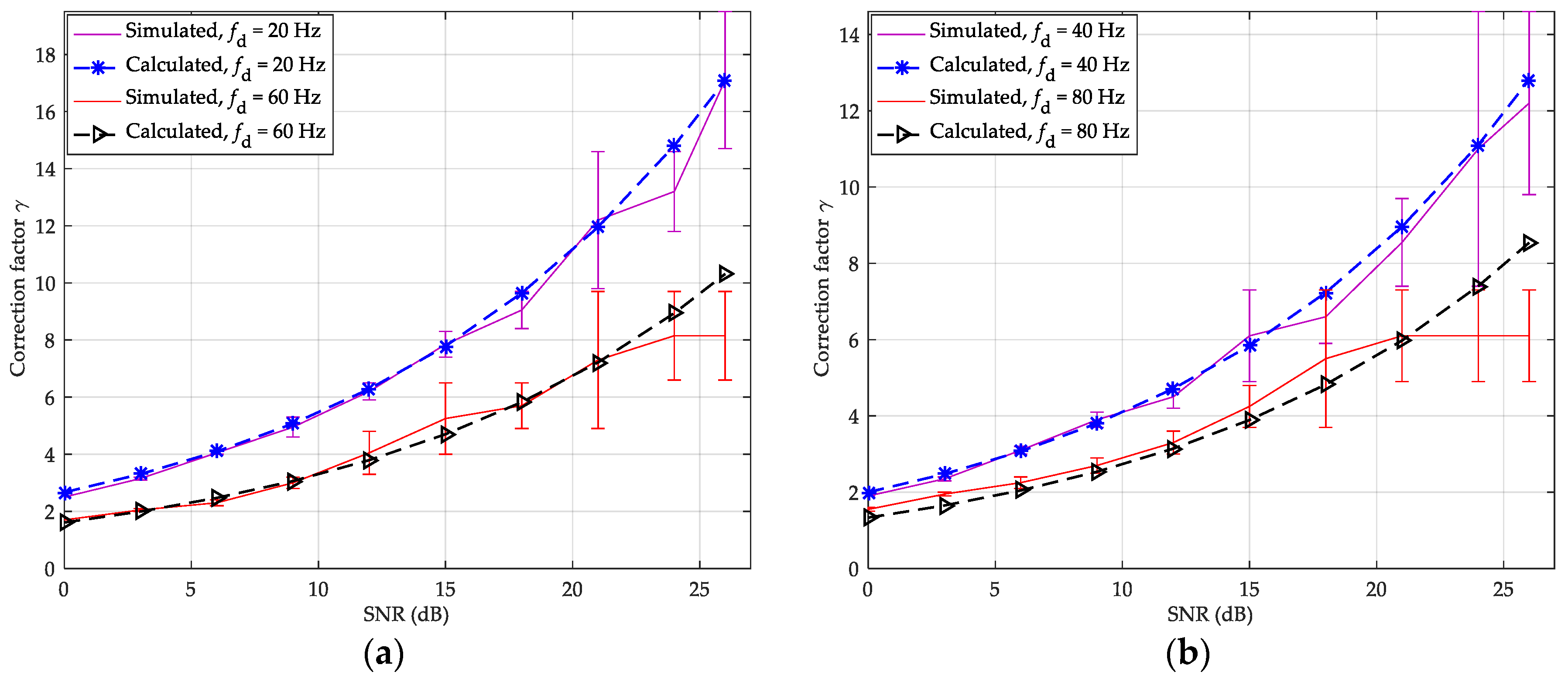
Since $\mathrm{floor}(\cdot )$ is used in Equation (22), the optimal value of $\gamma$ corresponding to different $R$ and $f_{\mathrm{d}}$ is not limited to a strictly accurate number, but a fluctuation range, which relaxes the requirement for the estimation accuracy of $R$ and $f_{\mathrm{d}}$. This can be expressed as Figure 3, whereby the fluctuation range of the optimal value of $\gamma$ corresponding to different $R$ and $f_{\mathrm{d}}$ are indicated by the vertical bars. Noted that the optimal value of $\gamma$ simulated in Figure 3 (solid line) is obtained by searching step by step with step length 0.1 according to Equation (22). It can be observed that there is an approximate exponential function relationship between $\gamma$ and $R$, and the exponential curve shifts up and down with the increase and decrease of $f_{\mathrm{d}}$. Therefore, after data fitting, this paper uses Equation (23) to fit the exponential function relationship, and it is fine-tuned by $f_{\mathrm{d}}$. Thus $\gamma$ can be expressed as:

$$\gamma =\rho {\mathrm{e}}^{\frac{R}{14}}\left[1+\frac{1}{3}{\log }_2(\frac{40}{f_{\mathrm{d}}})\right],$$

(23)

where ρ is a parameter related to the weight of the averaging frames and it is selected as $\rho =2$ for the proposed AWA method.

In Figure 3, the legend of “Calculated” means the value of $\gamma$ calculated from Equation (23). It can be seen that the Equation (23) can be acceptable for $R\in [0,25]\hspace{0.17em}\mathrm{dB}$ and low to medium Doppler spread conditions according to simulation. Therefore, combining Equations (22) and (23), the average frame number $B$ can be determined as:

$$B=\mathrm{floor}\left[\frac{0.537}{\rho {\widehat{f}}_{\mathrm{d}}T}{\mathrm{e}}^{-\frac{\widehat{R}}{14}}{\log }_2(\frac{{\widehat{f}}_{\mathrm{d}}}{320})\right].$$

(24)

5.2. The Process of Weighted Averaging

Through a large number of simulation experiments, if the weight of each frame for averaging is always one (i.e., unweighted), the parameter $\rho$ in Equation (23) should be $\rho =2.6$. The adaptive unweighted averaging (AUA) of multi-frame channel coefficients can be expressed as:

$${\widehat{\mathit{H}}}_{\mathrm{U}}(k,n)=\frac{1}{M_1}{\displaystyle \sum _{i=n-M_1+1}^{M_1}{\widehat{\mathit{H}}}_{\mathrm{T}}(k,i)},\hspace{1em}1\le k\le N,\hspace{0.17em}1\le n\le N_{\mathrm{t}},$$

(25)

where $M_1=\min [{\mathrm{B}}_1,n]$, $B_1$ is obtained by putting $\rho =2.6$ into Equation (24).

Considering that the correlation between two frames is inversely proportional to the distance, a weighting factor can be introduced to correct the weighted value of each frame in the averaging process. The estimated CFR in the AWA channel estimation method can be expressed as:

$${\widehat{\mathit{H}}}_{\mathrm{W}}(k,n)=(1/{\displaystyle \sum _{i=1}^{M_2}i}){\displaystyle \sum _{i=1}^{M_2}[i{\widehat{\mathit{H}}}_{\mathrm{T}}(k,n-M_2+i)]},\hspace{1em}1\le k\le N,\hspace{0.17em}1\le n\le N_{\mathrm{t}},$$

(26)

where $M_2=\min [B_2,n]$, $B_2$ is obtained by putting $\rho =2.0$ into Equation (24). It can be observed from Equation (26) that the frame used for averaging has a greater weight if it is closer to the current frame, which can better combat the negative effect of the Doppler spread and ICI.

In the AWA channel estimation method, since the channel is almost flat within the time interval $T_{\mathrm{B}}=B\times T$, the distortion brought by the Doppler spread and ICI can be neglected, and Equation (26) can be re-written as:

$${\widehat{\mathit{H}}}_{\mathrm{W}}(k,n)=\mathit{H}(k,n)+\frac{2}{M_2(M_2+1)}{\displaystyle \sum _{i=1}^{M_2}\left[i\mathit{W}(k,n-M_2+i)\right]},\hspace{1em}1\le k\le N,\hspace{0.17em}1\le n\le N_{\mathrm{t}}.$$

(27)

Because $\mathit{W}~\mathcal{C}\mathcal{N}(0,{\sigma }_{\mathrm{r}}^2{\mathit{I}}_N)$, the variance of the noise term in Equation (27) can be expressed as:

$${\sigma }_{\mathrm{W}}^2={\sigma }_{\mathrm{r}}^2{\left[1/{\displaystyle \sum _{i=1}^{M_2}i}\right]}^2{\displaystyle \sum _{i=1}^{M_2}{i}^2}=\frac{{\sigma }_{\mathrm{r}}^2(4M_2+2)}{3M_2(M_2+1)}.$$

(28)

Since $B_2\ll N_{\mathrm{t}}$ in practice, the assumption $M_2=B_2$ can be accepted and the noise suppression ratio of the AWA method is approximately equal to $(4B_2+2)/[3B_2(B_2+1)]$.

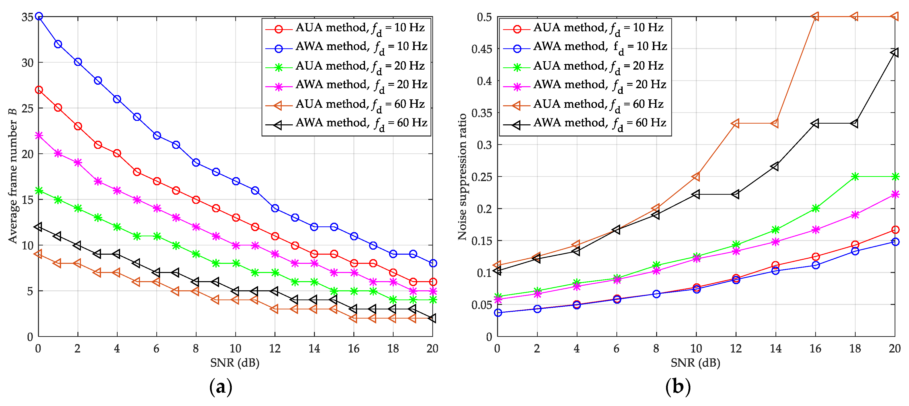
In the same way, the noise suppression ratio of the AUA method can be obtained from Equation (25), and it is approximately equal to $1/B_1$. The theoretical average frame number $B$ and noise suppression ratio of the AWA and AUA methods under different SNR and Doppler spread are presented in Figure 4.

In Figure 4a, with the increase of the SNR and Doppler spread, the theoretical average frame number of the AWA and AUA methods is all decreasing. Under the same condition, the AWA method has a more average frame number than the AUA method. Therefore, although the noise suppression effect of the AWA method is slightly worse under the same average frame number, its final noise suppression effect is stronger than the AUA method, which can be seen from Figure 4b. At the noise suppression ratio of 0.1, 0.2, and 0.3, the AWA method has about 0.6 dB, 2.5 dB, and 3.8 dB SNR gains compared with AUA method for $f_{\mathrm{d}}$ equal to 10 Hz, 20 Hz, and 60 Hz, respectively. It can be seen that the SNR gains increase with the increase of Doppler spread, which is because the AWA method can better combat the negative effect of the Doppler spread and ICI.

According to Equation (27), the proposed method mainly increases the addition operation and storage resources, so its computational complexity is in the same order as the threshold value method. Therefore, the proposed method is convenient for hardware implementation in practice.

6. Simulation Results and Performance Analysis

In this section, the simulation experiments are presented to demonstrate the performance of the proposed AWA-based noise suppression channel estimation method. The simulation is performed in static and dynamic multipath environments, respectively. The multipath channel models are China digital television (DTV) Test 1st (CDT1), CDT6, Brazil A, Brazil B, and Brazil D, where CDT1 and CDT6 channels are from the field tests for digital terrestrial television broadcasting (DTTB) in China and Brazil A, Brazil B, and Brazil D [19] channels are from the field tests for DTTB in Brazil [33]. These five channels are typical multipath broadcasting channel models, and all belong to the Rayleigh fading channel. CDT1 and Brazil A channels have slight frequency selectivity; CDT6, Brazil B, and Brazil D channels have stronger frequency selectivity.

The profiles for the Brazil A, Brazil B, and Brazil D channel models are shown in

Table 1. Profiles for Brazil A, Brazil B, and Brazil D channel models.

Tap	Brazil A		Brazil B		Brazil D
	Delay (μs)	Power (dB)	Delay (μs)	Power (dB)	Delay (μs)	Power (dB)
1	0	0	0	0	0	−0.10
2	0.15	−13.80	0.30	−12	0.48	−3.90
3	2.22	−16.20	3.50	−4	2.07	−2.60
4	3.05	−14.90	4.40	−7	2.90	−1.30
5	5.86	−13.60	9.50	−15	5.71	0
6	5.93	−16.40	12.70	−22	5.78	−2.80

. The profiles for the CDT1 and CDT6 channel models are shown in

Table 2. Profiles for China digital television (DTV) Test 1st (CDT1) and CDT6 channel models.

Tap	CDT1		CDT6
	Delay (μs)	Power (dB)	Delay (μs)	Power (dB)
1	0	0	0	0
2	−1.8	−20	−18	−10
3	0.15	−20	−1.80	−20
4	1.80	−10	0.15	−20
5	5.70	−14	1.80	−10
6	18	−18	5.70	−14

. The main simulation parameters for the OFDM system are presented in

Table 3. Simulation parameters of the OFDM system.

Parameters	Specifications
System model	CP-OFDM
Baseband symbol rate	7.56 × 106 symbols per second (SPS)
Modulation mode	QPSK
The number of OFDM frame	400
Subcarrier number	1152
CP length (subcarriers)	192
Pilot interval (subcarriers)	3
Doppler spread	20/40/60/80 Hz
Suppression factor $\alpha$	0.997 (20/40 Hz)/0.999 (60/80 Hz)

.

The performance of channel estimation is evaluated in terms of BER and NMSE, and the NMSE is defined as [26]:

$$\mathrm{NMSE}=\sqrt{{\displaystyle \sum _{n=1}^L{\left[{\hat{\mathit{h}}}_i(n)-{\mathit{h}}_i(n)\right]}^2}/{\displaystyle \sum _{n=1}^L{\left[{\mathit{h}}_i(n)\right]}^2}},$$

(29)

where ${\widehat{\mathit{h}}}_i(n)$ and ${\mathit{h}}_i(n)$ represent the estimated CIR by various channel estimation methods and real CIR in the i-th frame, respectively. BER reflects the overall performance of the wireless communication system, NMSE reflects the estimation accuracy of various channel estimation methods. They are the two most commonly used indicators in the field of channel estimation.

The conventional LS, threshold value, IMMSE, and the proposed AWA and AUA channel estimation methods are presented in the CP-OFDM system. Moreover, an ideal channel estimation (ICE) method is given in the simulation results, which is the channel estimation with the known channel coefficients, as a reference. In the CP-OFDM system, the number of total subcarriers is 1152, and the CP occupies 192 subcarriers. Therefore, the total number of actual application subcarriers including pilot and data is $N=1152-192=960$, where $N_{\mathrm{P}}=N/4=240$ comb-type pilot subcarriers are employed. For both pilots and data, the symbols are drawn from a QPSK constellation. The baseband symbol rate of the CP-OFDM system is $7.56\times {10}^6$ symbols per second and the duration of each OFDM frame is $\mathrm{T}=1152/7.56\times {10}^{-6}\hspace{0.17em}\mathrm{s}=152.38\hspace{0.17em}\mathsf{\mu }\mathrm{s}$. In dynamic multipath environments, Doppler spread is chosen to be 20 Hz, 40 Hz, 60 Hz, and 80 Hz, respectively. According to [27], the suppression factor $\alpha$ in the IMMSE method is 0.997 for a Doppler spread equal to 20 Hz or 40 Hz and 0.999 for a Doppler spread equal to 60 Hz or 80 Hz, which can suppress the AWGN effectively with a smaller loss of the partial path energy. For a better study of the performance of the proposed method, neither interleaving methods nor any channel coding techniques are used.

6.1. The Performance in Static Channel

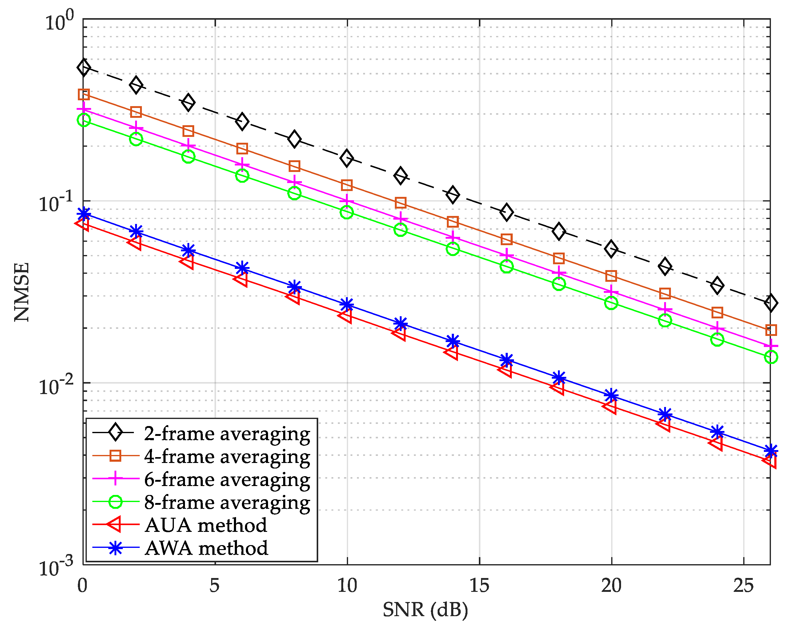
The NMSE performance of fixed and adaptive multi-frame averaging methods under a static CDT1 channel is shown in Figure 5. The BER and NMSE performance of LS, threshold value, IMMSE, and the proposed channel estimation methods under static CDT6 channel are shown in Figure 6 and Figure 7, respectively.

As can be seen from Figure 5, the NMSE of the six channel estimation curves all decreases with the increase of the SNR. For fixed multi-frame averaging method, the NMSE decreases with the increase of the average frame number. In Figure 5, the AUA method has the best NMSE performance, which is slightly better than the AWA method. The reason is that there is no Doppler spread in the static channel, and the advantage of weighted averaging against the negative effect of the Doppler spread and the ensuing ICI cannot be reflected. At the NMSE of $5\times {10}^{-2}$, the proposed AUA method can provide about 0.9 dB and 11.2 dB SNR gains compared with the AWA and fixed 8-frame averaging methods, respectively. Moreover, the gaps of the SNR gain among fixed 8-frame, 6-frame, 4-frame, and 2-frame averaging methods is about 1.2 dB, 1.7 dB, and 3.1 dB at the NMSE of $5\times {10}^{-2}$, respectively. Therefore, under the static CDT1 channel, the proposed adaptive averaging method is much better than the fixed averaging method.

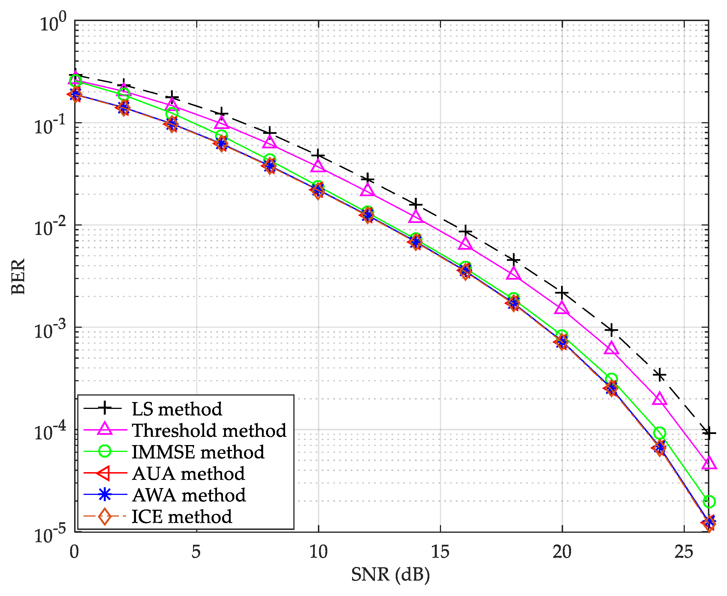
In Figure 6, the proposed AUA and AWA methods have almost the same BER performance, and both of them can improve the channel estimation performance in the overall SNR range similar to the ICE method. The reason is that there is no distortion caused by averaging under the static channel. Compared with the IMMSE, threshold value, and LS methods, the proposed AWA method has about 0.3 dB, 1.6 dB, and 2.6 dB SNR gains at the BER of ${10}^{-3}$. It can be seen that AWGN is the main factor affecting the accuracy of channel estimation, and the noise effect can be significantly suppressed by the proposed AWA method under the static CDT6 channel.

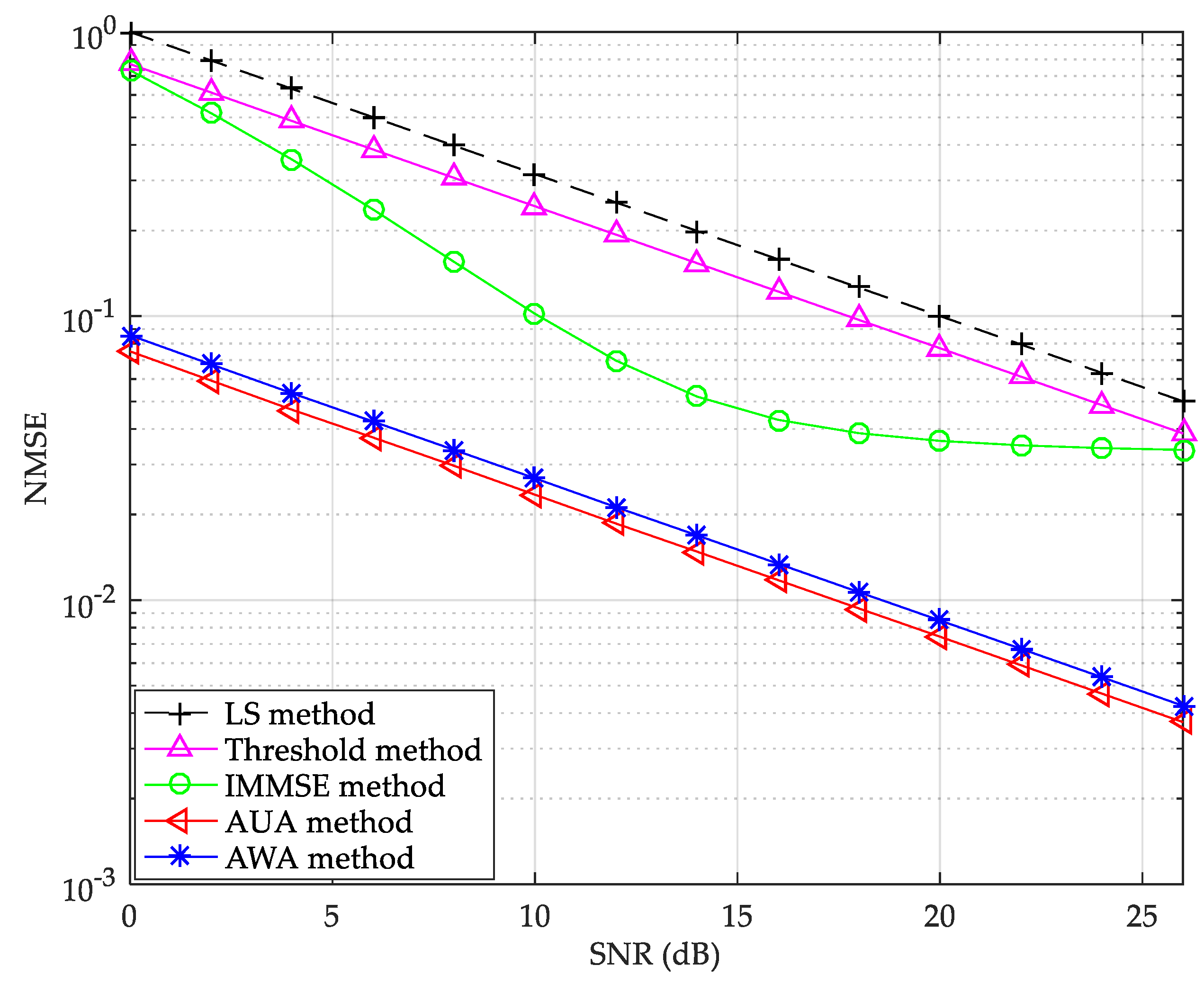
In Figure 7, the proposed AUA method has the best NMSE performance, and it can provide about 0.9 dB and 10.6 dB SNR gains compared with the proposed AWA method and IMMSE method at the target NMSE of $5\times {10}^{-2}$. Meanwhile, the gaps of the SNR gain among the IMMSE, threshold value, and LS methods are about 8.1 dB and 1.1 dB at the NMSE of $5\times {10}^{-2}$, respectively. This is because the average frame number of the AWA method is the same as that of the AUA method under the static channel, and the noise suppression ability of the AWA method is slightly worse under the same average frame number, which can be seen from Equation (28). Although the NMSE performance of the AUA method is slightly better than that of the AWA method in the static CDT6 channel, the BER performance of these two methods is almost identical, which can be seen from Figure 6. Therefore, in the static scenarios, the weight has little influence on the proposed adaptive averaging method.

6.2. The Performance in Dynamic Channel

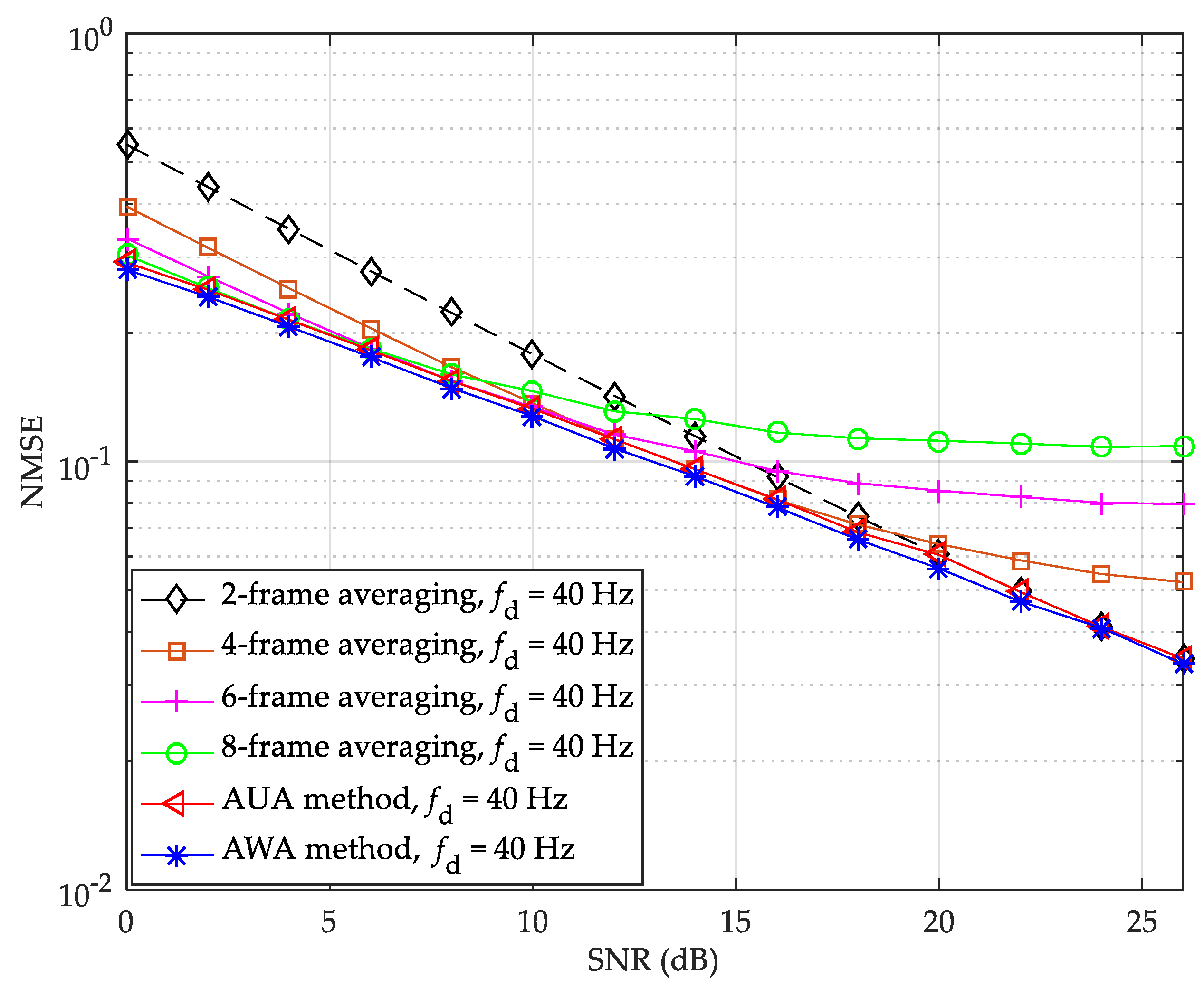
The NMSE performance of fixed and adaptive multi-frame averaging methods under Brazil A channel with Doppler spread 40 Hz is shown in Figure 8. The BER and NMSE performance of the LS, threshold value, IMMSE, and the proposed channel estimation methods under Brazil A channel with Doppler spread 20 Hz are shown in Figure 9 and Figure 10, respectively.

In Figure 8, the proposed AWA method has the best NMSE performance and the fixed multi-frame averaging method is not suitable for dynamic channel scenarios. When the SNR increases, the performance of the fixed multi-frame averaging method in the dynamic channel deteriorates dramatically, and the more frames used in the fixed averaging method, the worse the performance deteriorates. In particular, the NMSE performance of the fixed 8-frame averaging method begins to deteriorate when the SNR is only greater than 10 dB. In the overall SNR range, the AWA method has about 0.5 dB SNR gains compared with the AUA method. This is because the AWA method allows the average frames to be weighted by their distance from the current frame, enabling more relevant average frames to play more dominant roles in the averaging process, and thus better combat the negative effect of the Doppler spread and ICI.

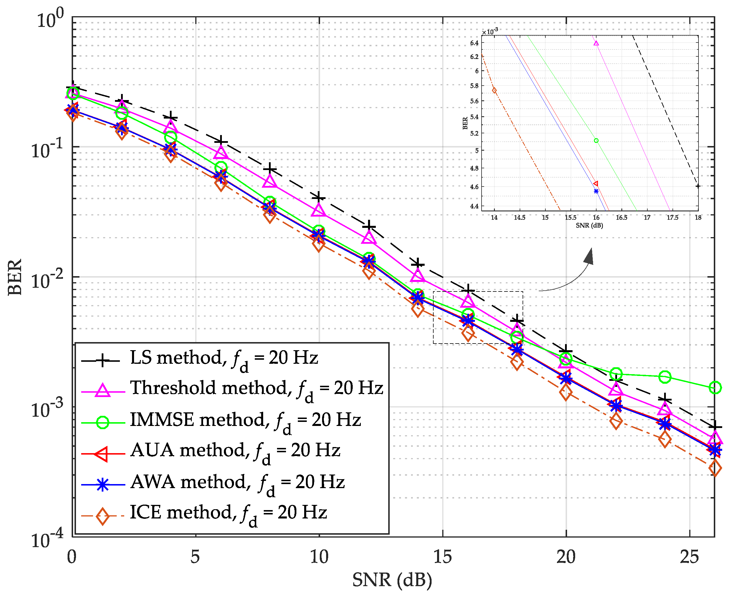
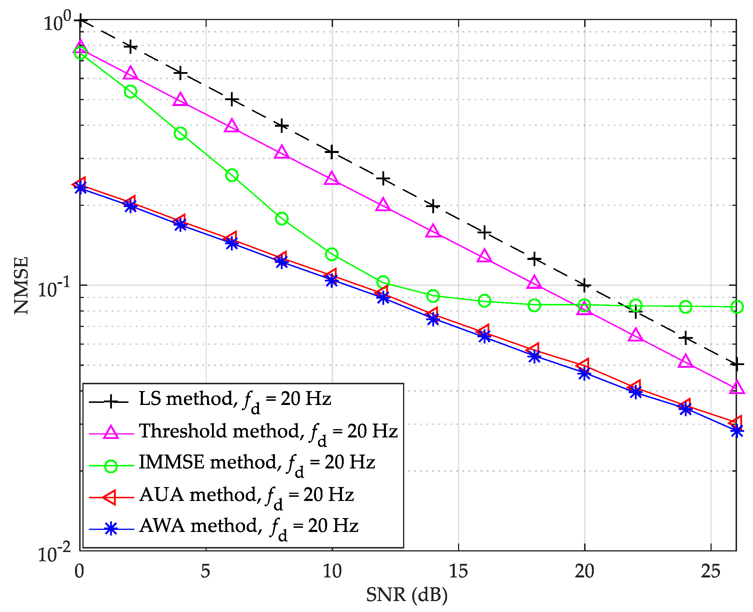
As shown in Figure 9 and Figure 10, the proposed AWA method provides better NMSE performance as well as system BER than the other channel estimation methods except the ICE method. For example, in Figure 9, at the BER of 5 × 10⁻³, compared with the ICE method, the proposed AWA method has about 0.8 dB SNR degradation, compared with the AUA, IMMSE, threshold value, and LS methods, the proposed AWA method has about 0.1 dB, 0.6 dB, 1.4 dB, and 2.1 dB SNR gains, respectively. In Figure 10, at the NMSE of 10⁻¹, compared with the AUA, IMMSE, threshold value, and LS methods, the proposed AWA method has about 0.5 dB, 1.8 dB, 7.4 dB, and 9.3 dB SNR gains, respectively. Thus, the proposed adaptive averaging-based noise suppression channel estimation method works well under Brazil A channel with Doppler spread 20 Hz, and its performance can be further improved by introducing weighting factor to combat the distortion caused by Doppler spread and ICI.

The BER and NMSE performance of the LS, threshold value, IMMSE, and the proposed channel estimation methods under Brazil B channel with Doppler spread 60 Hz are shown in Figure 11 and Figure 12, respectively.

By comparing Figure 9 and Figure 10 with Figure 11 and Figure 12, it can be seen that the performance under Brazil B channel is worse than Brazil A channel, which is because Brazil B channel has stronger frequency selectivity and Doppler spread than Brazil A channel. However, the proposed AWA method still has the best performance among the six channel estimation methods except the ICE method. In Figure 11, the proposed AWA method can provide about 0.2 dB, 0.3 dB, 1.1 dB, and 1.8 dB SNR gains, and has about 1.1 dB SNR degradation, compared with the AUA, IMMSE, threshold value, LS, and ICE methods at the BER of 10⁻², respectively. Therefore, with the increase of Doppler spread, the AWA method has more obvious advantages over the AUA method. In Figure 12, the IMMSE method has bad NMSE performance when the SNR is higher than 18 dB. This is because the IMMSE method suffers from a loss of the partial path energy while suppressing the noise effect. At the NMSE of 10⁻¹, the proposed AWA method has about 0.5 dB, 1.5 dB, 4.1 dB, and 5.6 dB SNR gains compared with the AUA, IMMSE, threshold value, and LS methods, respectively. It can be seen that the proposed AWA method effectively suppresses the residual noise in the threshold value channel estimation and greatly improves the accuracy of channel estimation.

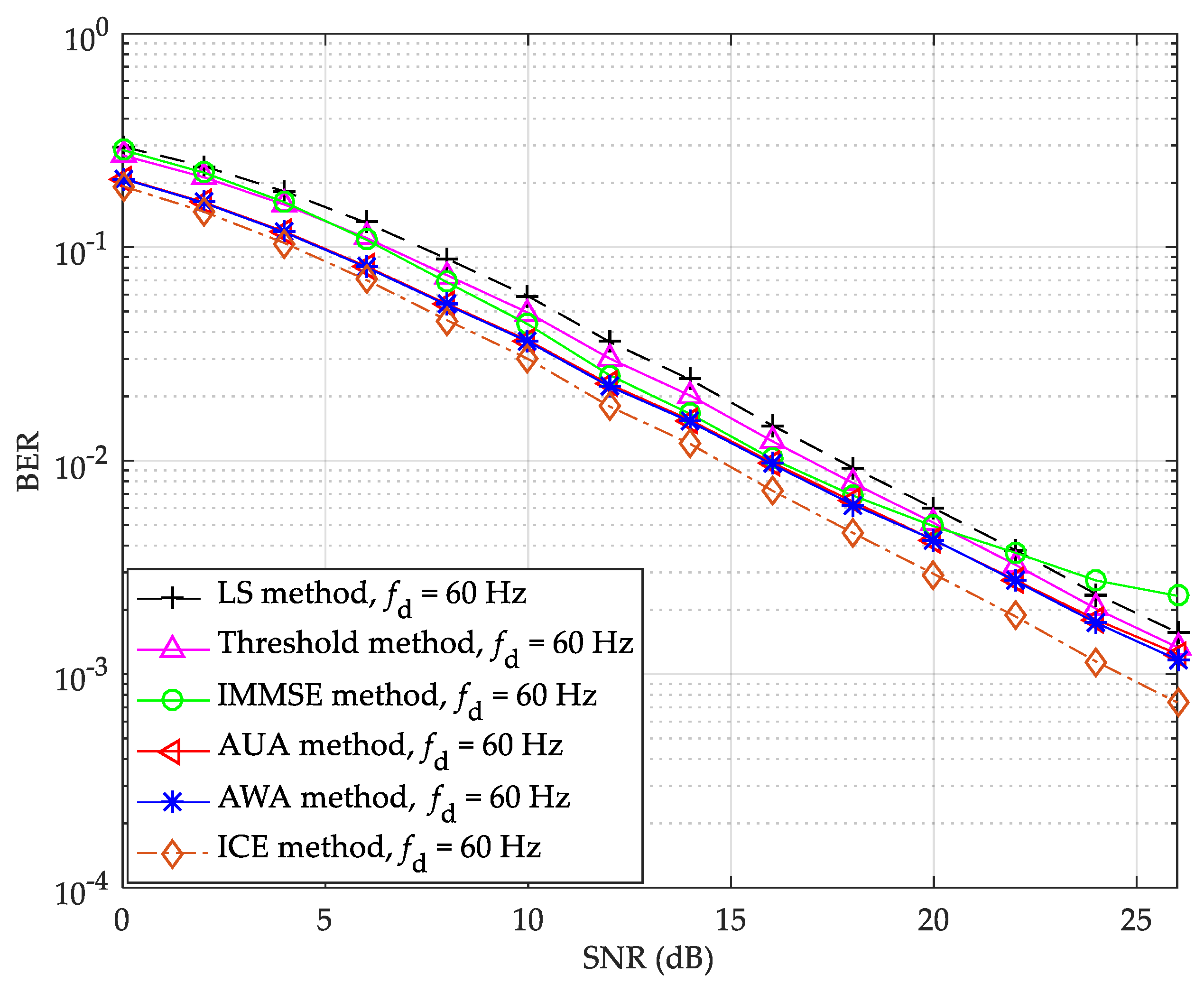
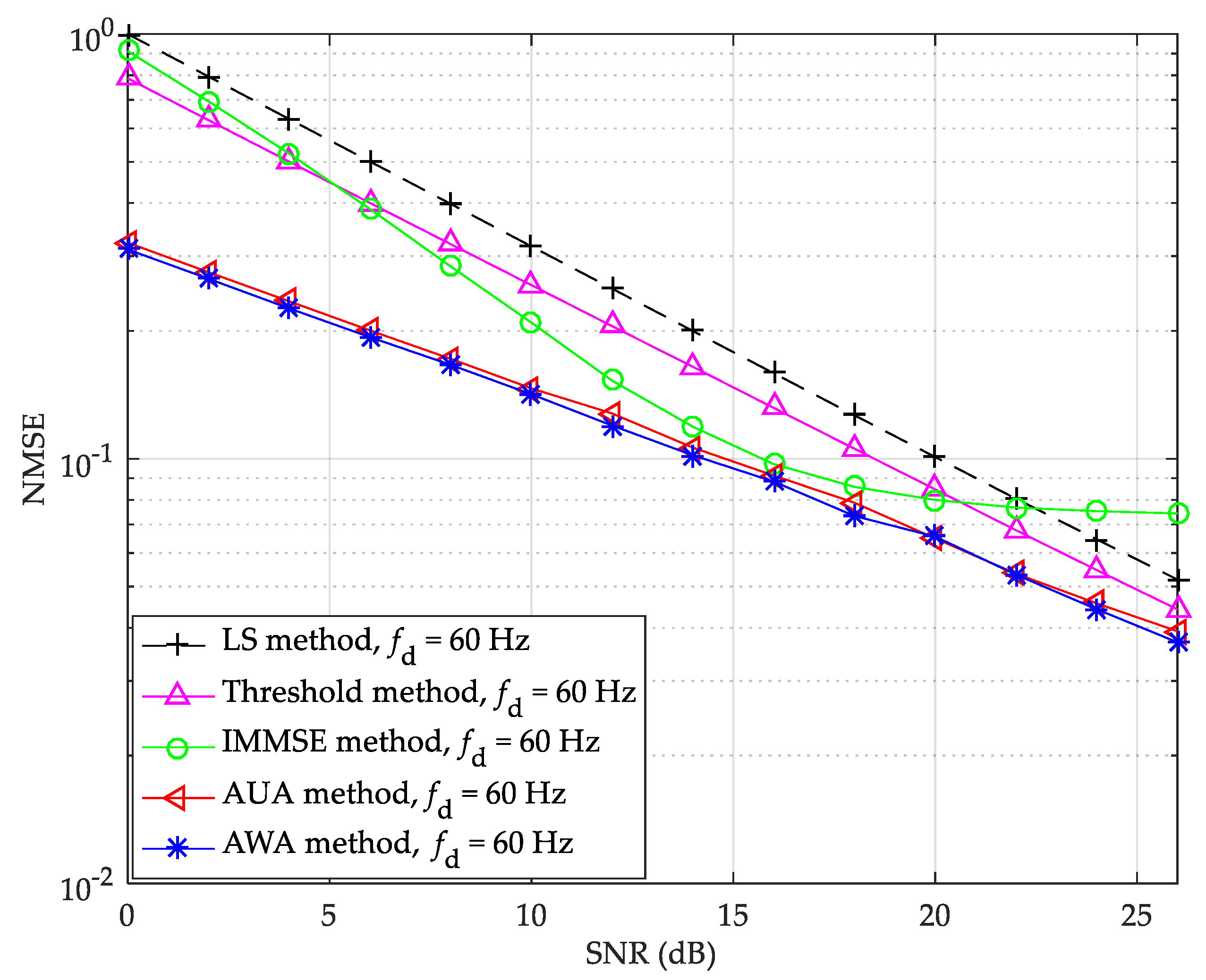
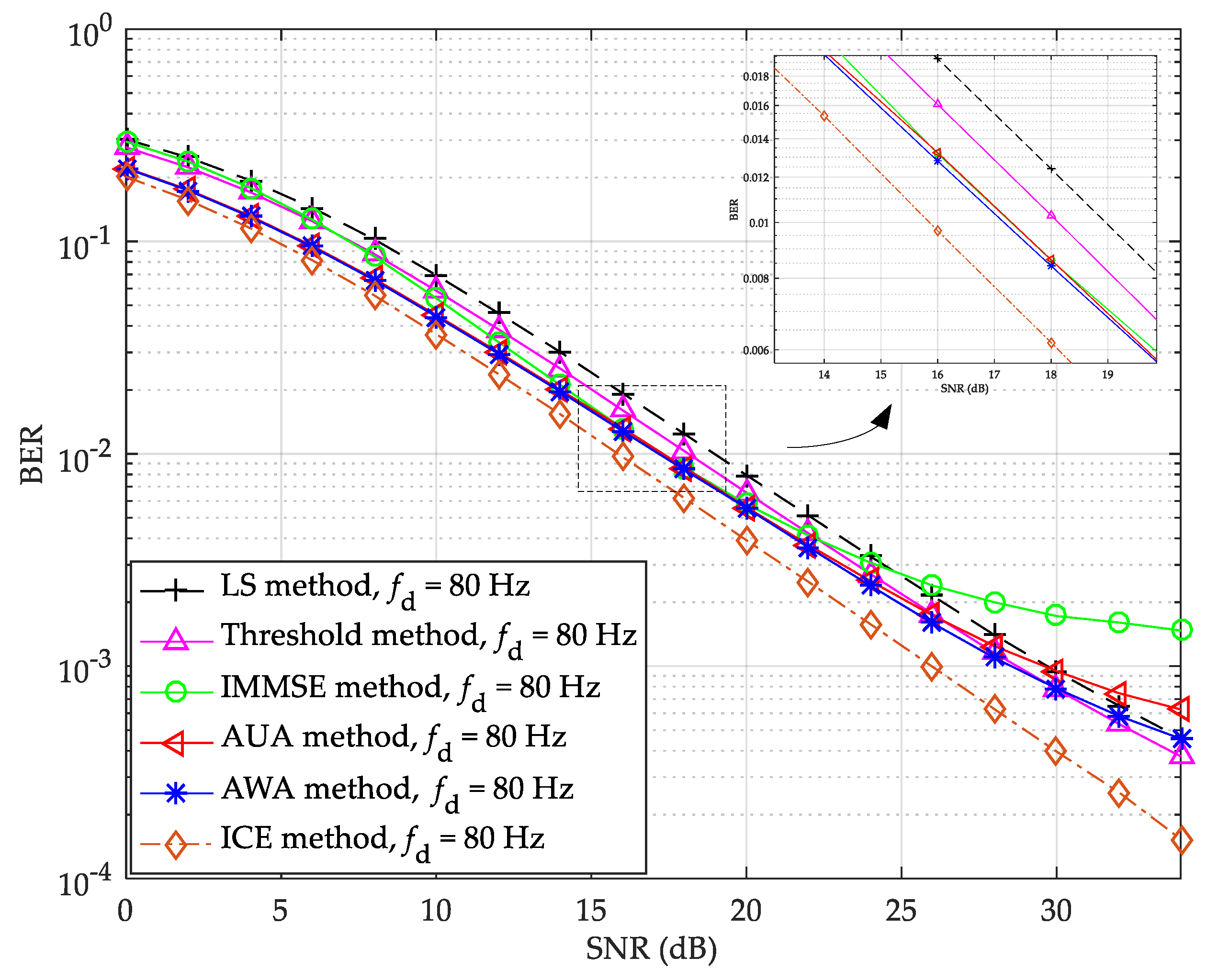
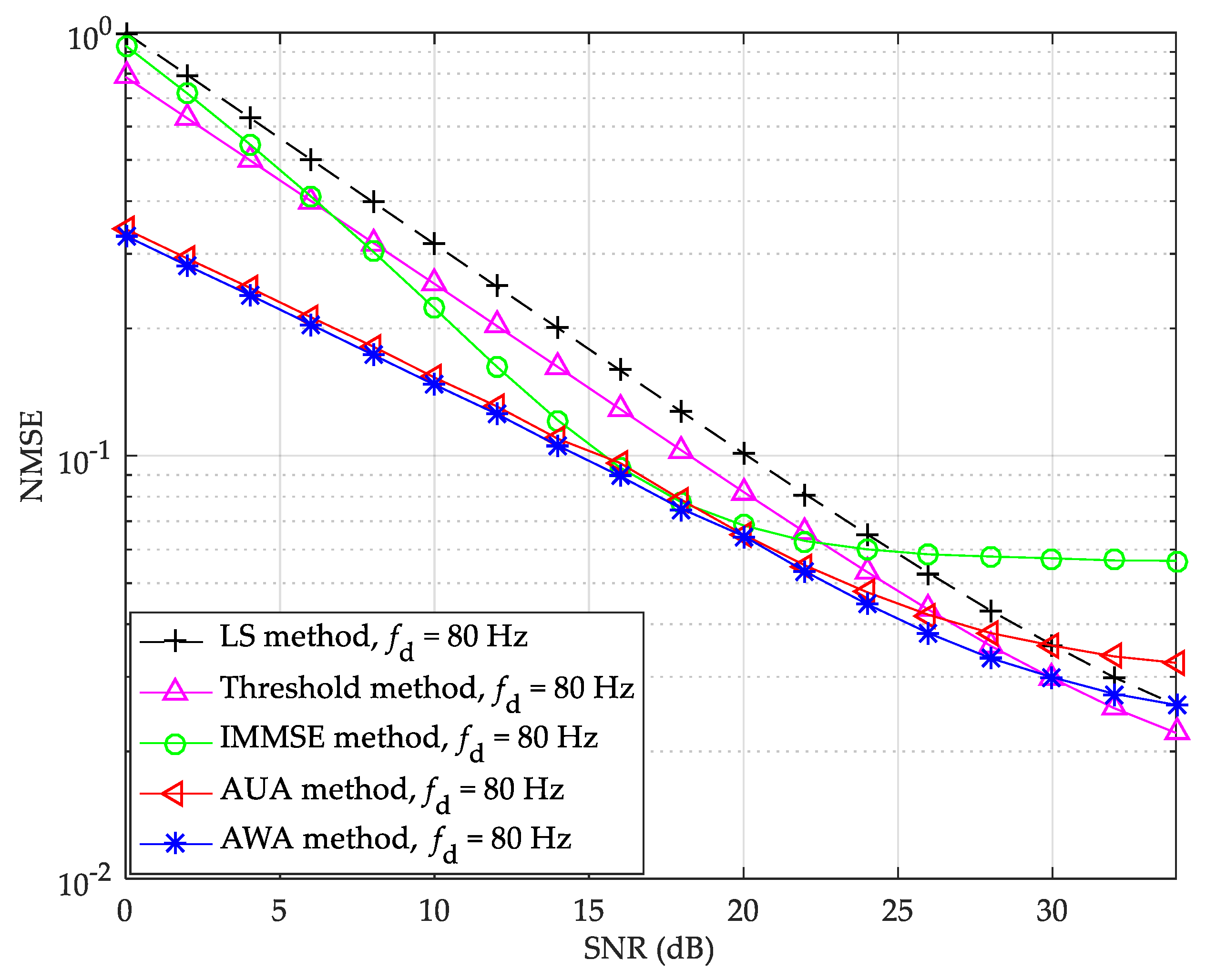
The BER and NMSE performance of the LS, threshold value, IMMSE, and the proposed channel estimation methods under Brazil D channel with Doppler spread 80 Hz are shown in Figure 13 and Figure 14, respectively.

In Figure 13 and Figure 14, the IMMSE method has bad BER and NMSE performance when the SNR is higher than 20 dB, and the proposed AWA method has the best BER and NMSE performance when the SNR is lower than 30 dB. In Figure 13, the proposed AWA method can provide about 0.1 dB, 0.1 dB, 0.9 dB, and 1.7 dB SNR gains, and has about 1.0 dB SNR degradation, compared with the AUA, IMMSE, threshold value, LS, and ICE methods at the BER of 10⁻², respectively. In Figure 14, at the NMSE of 10⁻¹, the proposed AWA method has about 0.8 dB, 0.9 dB, 3.7 dB, and 5.4 dB SNR gains compared with the AUA, IMMSE, threshold value, and LS methods, respectively. However, when the SNR is greater than 30 dB, the performance of the proposed AWA method is no longer optimal. This is because the noise effect is small in the high SNR and Doppler spread scenarios, and the channel distortion brought by the averaging becomes significant.

7. Conclusions

In this paper, we studied the multi-frame averaging scheme in the frequency domain for channel estimation and proposed an adaptive weighted averaging-based noise suppression channel estimation method. Combined with the Doppler spread and SNR information, the proposed method can adaptively select the average frame number, so it can adapt to the dynamic channel. Moreover, the introduction of weights improves the robustness of the proposed method to the Doppler distortion. Specially, the proposed method can be combined with other conventional noise suppression methods, such as the threshold value method in this paper, to further eliminate the residual noise effect existing in the channel estimation results, and significantly improve the channel estimation accuracy. Simulation results show that the proposed channel estimation method can provide a good performance under static and dynamic multipath channels. Yet under the dynamic channels with very large Doppler spread and SNR, the performance of the proposed adaptive weighted averaging method needs to be further improved.

Compared with the conventional LS, IMMSE, and threshold value methods, the proposed adaptive weighted averaging-based noise suppression channel estimation method has the best BER and NMSE performance. Meanwhile, the proposed method has the same order computational complexity as the threshold value method, so it can be easily implemented in practice and has broad market prospects that can be applied in MIMO technique, OQAM technique, and cognitive radio technique.