1. Introduction
The rolling bearings are key components of rotary machines, but harsh working conditions often make them suffer from different failure, which may lead to the breakdown of the whole machinery and huge economic loss [
1,
2]. Therefore, it is of great significance to monitor the condition of the bearing. Vibration analysis has been widely applied to diagnose bearing faults. However, the faulty signal acquired from the bearing is usually weak or submerged in strong noise [
3,
4]. Traditional weak signal detection methods, such as empirical mode decomposition (EMD) [
5], wavelets transform (WT) [
6], singular value decomposition (SVD) [
7], and variational mode decomposition (VMD) [
8], mainly reduced noise to improve signal-to-noise ratio (SNR) and extract fault characteristics, which inevitably weakened useful fault signal characteristic information. In contrast, SR can utilize noise to enhance weak signal energy.
Stochastic resonance (SR) was proposed by Benzi in 1981 [
9], which have been applied in various fields. At present, SR has been used in bearing fault diagnosis. The adiabatic approximation theory of SR requires that the input signal frequency of the SR system is less than 1 Hz, while the fault characteristic frequency of the bearing is much larger than 1 Hz in practical engineering applications. To deal with this limitation, Leng [
10] proposed the re-scaling frequency SR and Tan [
11] presented the frequency-shifted and re-scaling SR. However, beyond that, He [
12] proposed a multi-scale noise tuning technique to overcome the limitation of small parameter requirement of the classical SR, and took advantage of the multiscale noise for an improved SR performance. These methods promoted the application of SR in practical engineering.
Scholars have proposed different SR models and parameter optimization algorithms in the field of the classical first-order SR system. Several bistable potentials have been proposed and applied in the detection of weak signals. Reference [
13] proposed the use of particle swarm optimization to achieve the selection of bistable stochastic resonance system parameters (CSR). Qiao [
14] established a new piecewise bistable potential model to overcome the disadvantage of output saturation of the CSR. Zhang [
15,
16] introduced a joint with Woods–Saxon and Gaussian potential, and step-varying asymmetric stochastic for bearing fault diagnosis. In multistable potentials, Li [
17] presented overdamped multistable SR with a tristable potential to extract the fault characteristics of the rolling mill gearbox and the detection results show that the multistable SR method has better processing effects than the classical bistable SR method for weak signals. Han [
18] proposed a multi-stable SR system for multi-frequency weak signal detection and Liu [
19] improved an adaptive SR with the periodic potential system using a trigonometric function. In short, SR with multistable potential has a better filtering performance than bistable SR. The other intelligent methods are proposed to apply in the field of fault diagnosis [
20,
21,
22].
Most of the research focused on the first-order SR system, however the filtering performance of the underdamped (second-order) SR system is much better than that of the first-order SR system, and the output SNR is higher. Lu [
23] proposed an underdamped step-varying second-order SR method (USSSR), verified the practicability by analyzing a set of defective bearing signals, and confirmed the effectiveness in comparison with a traditional SR method. López [
24] explored the second order SR with a FitzHug–Nagumo potential for weak signal detection. Lei [
25] presented an underdamped SR method with stable-state matching for incipient bearing fault diagnosis. Xia [
26] proposed an improved SR method with an arbitrary stable-state potential for incipient bearing fault diagnosis. Liu [
27] proposed a step-varying vibrational resonance (SVVR) method based on the duffing oscillator nonlinear system and concluded that the SVVR is more effective in extracting weak characteristic information than other methods. All in all, the second-order SR method is able to obtain higher output SNR and better performance than the first-order SR method.
Based on the abovementioned, a new second-order tristable SR method (STSR) method is proposed in this study based on the classical bistable potential and Woods–Saxon potential. This paper uses the re-scaling frequency method to detect large frequency weak signals, in which an R parameter is introduced. Since the parameters of the SR system determines its performance, we can use Seeker Optimization Algorithm (SOA) to solve multiple parameters synchronously. To evaluate the performance of the proposed STSR method, compare this method with traditional SR methods. It is proved by a simulation signal that the STSR method is more conducive to the detection of weak signals than traditional SR methods and obtains larger output SNR. Finally, the proposed method and traditional SR method are applied to fault diagnosis of bearings, respectively.
The remainder of this paper is organized as follows. The STSR model is introduced in
Section 2, the influence of the noise intensity
D and damping ratio
k on the STSR output signal are analyzed, and the process weak fault characteristic extraction based on SOA is presented.
Section 3 and
Section 4 use some data to verify the effectiveness of the proposed method.
Section 5 provides a summary of this paper.
2. STSR System
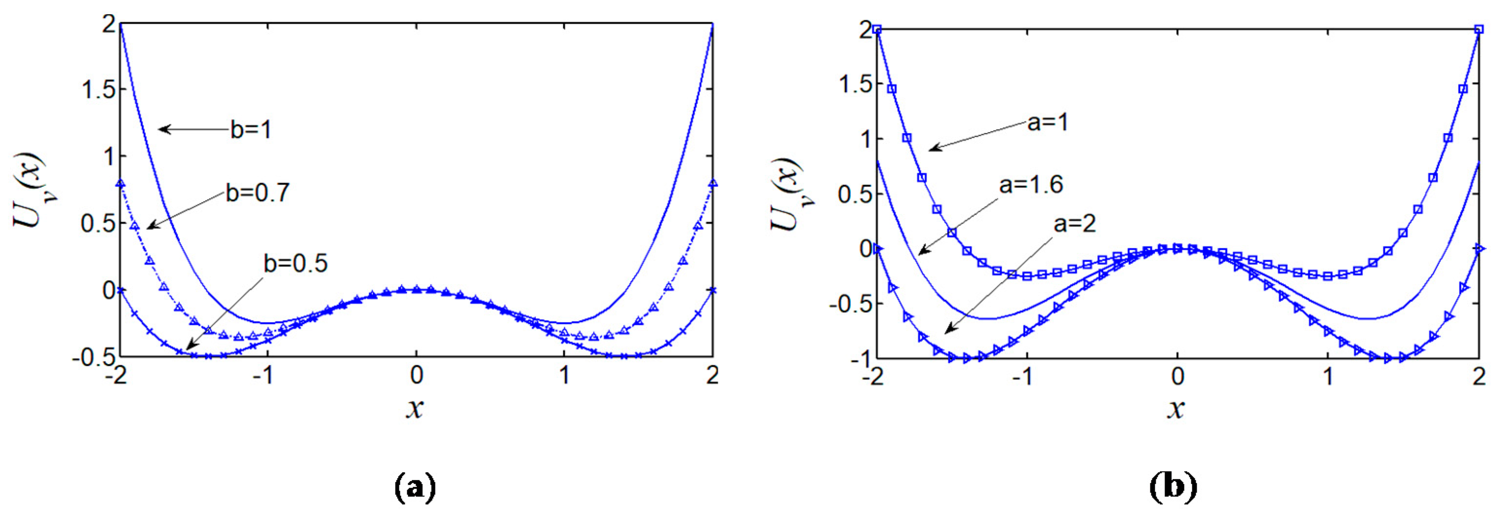
The bistable potential system is one of the classical SR models, where the function expression can be expressed as:
where
a and
b are real positive values.
Figure 1 shows the fixed parameters
a or
b, respectively, in order to analyze their influence on the potential barrier and the potential well.
It can be found that, when the fixed parameter
a = 1, the barrier height decreases with the increase of
b. Additionally, when the fixed parameter
b = 1, the barrier height increases with the increase of
a from
Figure 1. Thus, the parameters
a and
b affect the barrier height together. The traditional method of selecting parameters
a and
b manually, and fixing one parameter adjustment of another parameter neglects the coupling effect between the parameters, which may directly lead to the performance of SR detection in weak features detection.
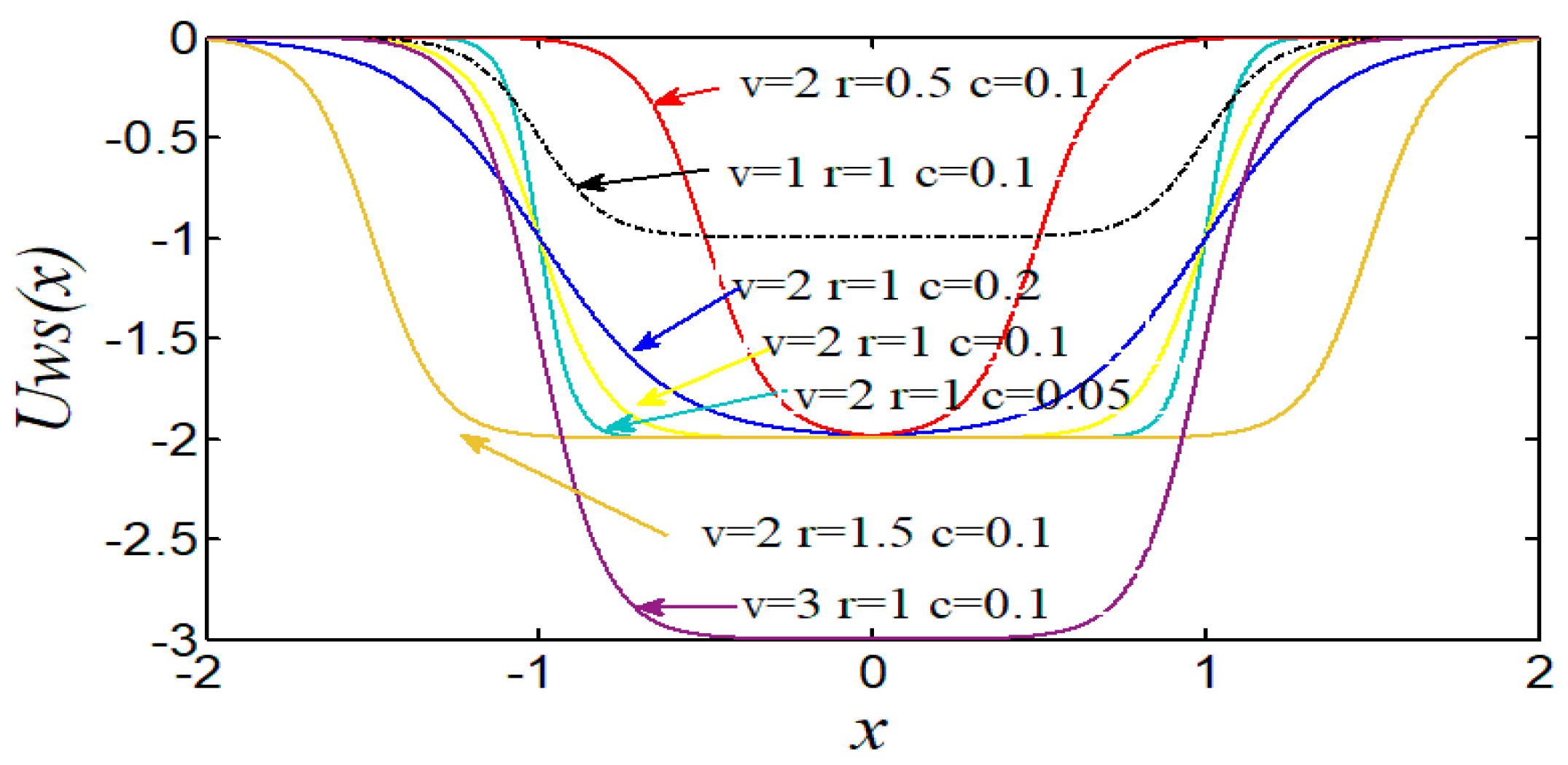
The Woods–Saxon potential (
Uws) [
28] is a nonlinear symmetric potential, proposed by Woods and Saxon.
Uws can be expressed as follows:
where parameter
V affects the depth of the potential and parameter
r works on the width of the potential, while parameter
c determines the wall steepness of the potential. These three parameters together determine the shape and performance of the potential.
Figure 2 shows the effect of different parameters on the shape of the potential function. When the parameters
V and
r are fixed, the potential well becomes slower as the
c increases; parameters
V and
c are fixed, the potential well function becomes wider as the r increases; and parameters
r and
c are fixed, the depth of the well becomes deeper as the
V increases. Thus, the shape of the potential well can be changed by adjusting the parameters.
2.1. Tristable Potential
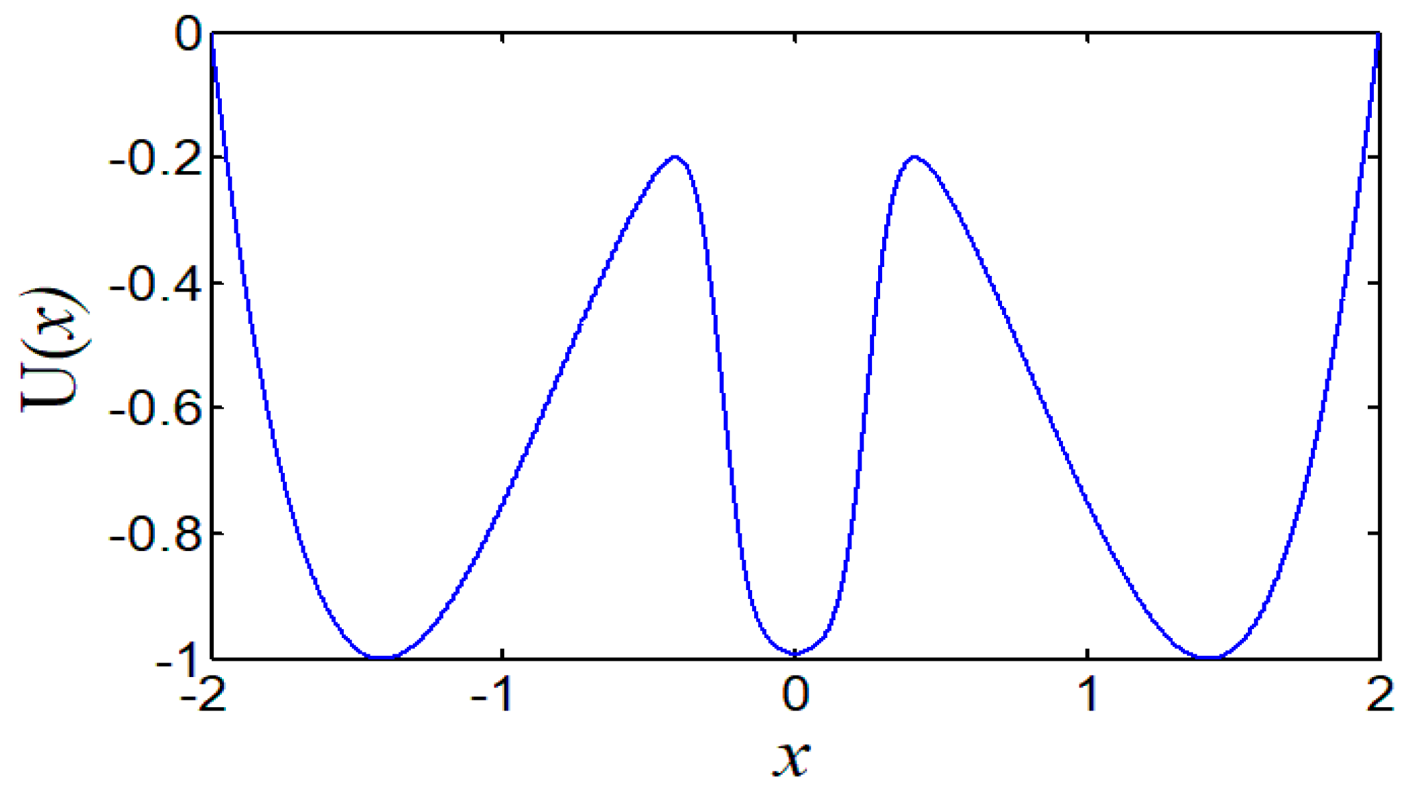
We established a new tristable potential model by the combination of Woods–Saxon potential and bistable potential based on the above introduction, which can be expressed as follows:
Set the potential parameters
a = 2,
b = 1,
V = 1,
r = 0.25, and
c = 0.05 to construct a new tristable potential function that is still a symmetric potential shown in
Figure 3. The parameters
a,
b,
c,
V and
r together determine the shape of the potential function. We can adjust the parameters in order to realize the potential function to become a monostable potential or a bistable potential and a tristable potential. Therefore, the proposed potential has the advantages of monostable potential, bistable potential, and tristable potential.
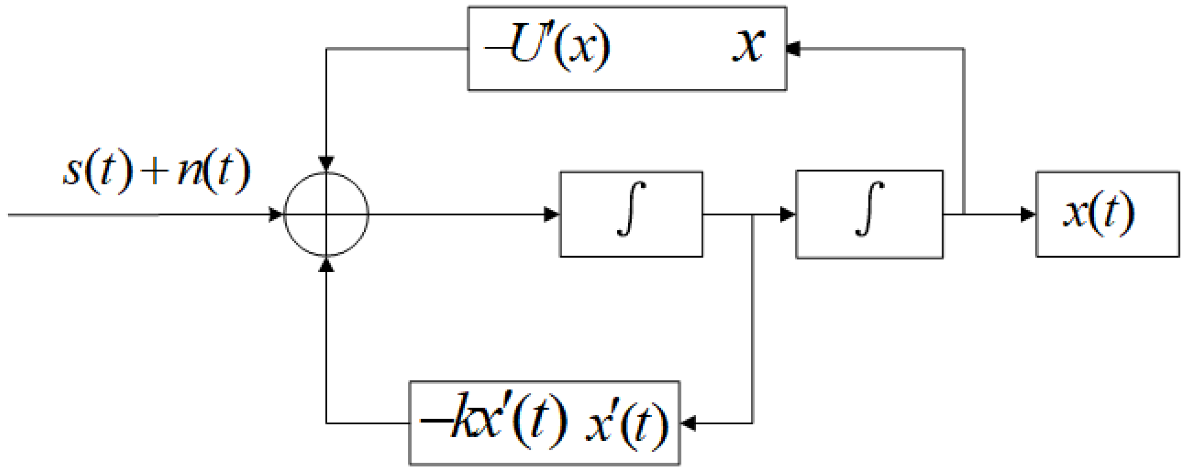
2.2. The STSR
The second-order SR system can be described as:
s(t) + n(t) is the input signal of the SR system, s(t) is a periodic signal, is the background noise, w(t)is the Gaussian noise, k is damping ratio, x represents the output signal of SR system, and U(x) is the potential proposed in this paper.
Substituting Equation (3) in Equation (4), the Equation of second-order SR based on the
U(
x) potential can be expressed as follows:
Equation (5) is the second-order tristable SR (STSR).
Figure 4 is a sketch that describes the STSR model. One integration can be regarded as a filtering process, so the output signal
x(
t) is obtained by second filtering, which provides better denoising performance than the first-order SR. The STSR system can be regarded as the output signal
x(
t) obtained by secondary filtering of the input signal
s(
t) +
n(
t), and the system parameters determine the filtering effect.
This paper splits Equation (5) into two first-order differential equations, and introduces the parameter
y,
, so Equation (4) can be rewritten as follows:
The solution process of Equation (6) can be expressed as follows:
where
x is STSR output signal and
h is the sampling interval.
2.3. Influence of Parameters on STSR and Procedure of STSR
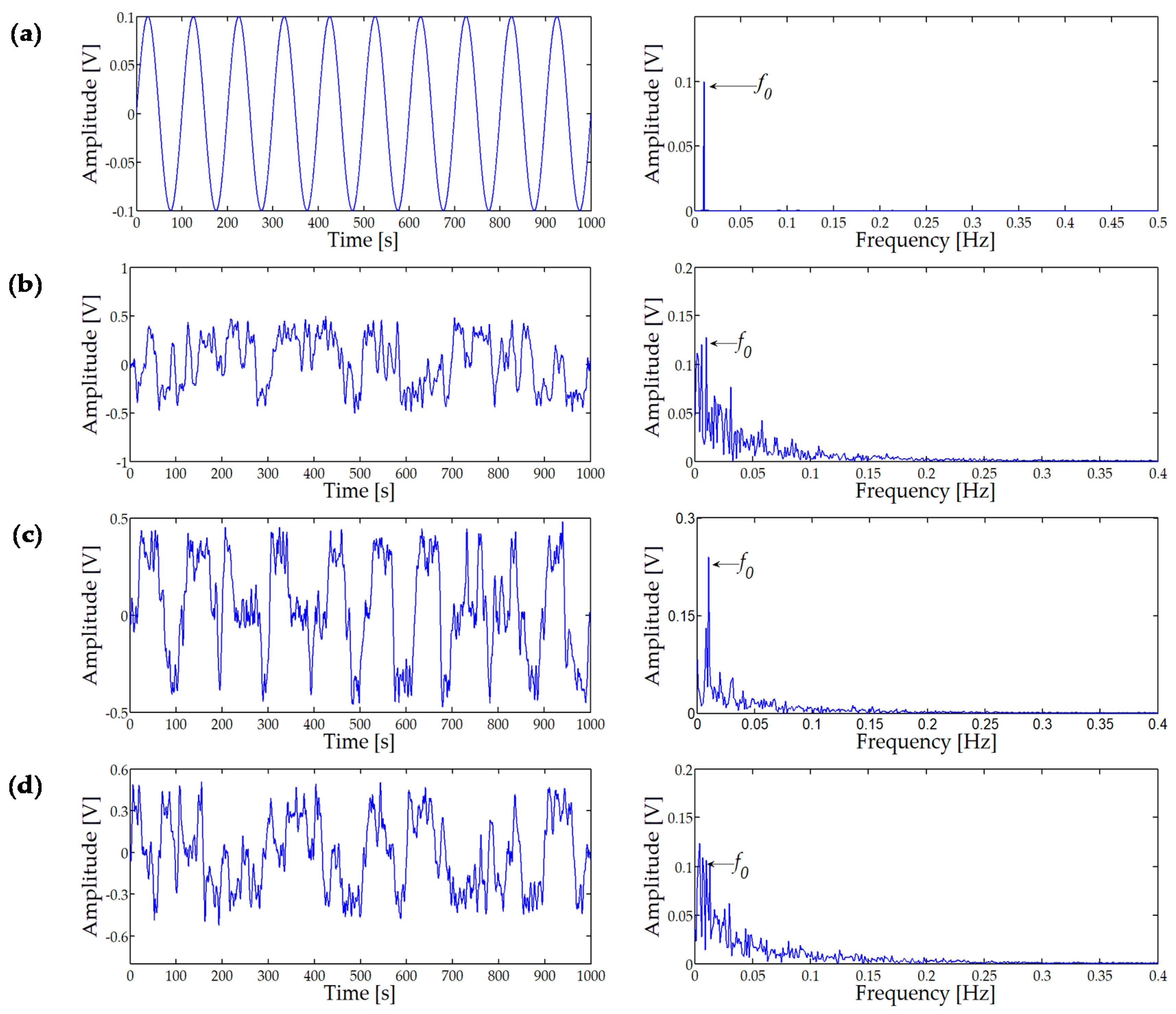
Firstly, the effect of noise intensity
D on STSR output signal is analyzed. Due to the adiabatic approximation theory of SR, the input signal amplitude
A, frequency
f0 meets the requirements of small parameters,
A < 1,
f0 < 1. Thus, we can simulate a small parameter signal to explore the effect of noise intensity
D on STSR. The simulation signal is defined as:
where
A = 0.1,
f0 = 0.01 Hz and
n(
t) is the zero mean Gaussian white noise.
Set the other parameters of the signal as follows: The sampling frequency is
fs = 5 Hz and the length of the signal
N = 5000. The time domain and amplitude spectrum of the signal without noise are shown in
Figure 5a. Here, given a set of parameters that can produce SR,
a = 0.4,
b = 2.7,
V = 11,
r = 39,
c = 20, and
k = 0.47. The time domain waveform and amplitude spectrum of the STSR output signal are shown in
Figure 5b when
D = 0.3, and the frequency 0.01 Hz cannot be seen. Further, adding noise to the input signal, as the noise increases, STSR obtains the output signal, as shown in
Figure 5c when
D = 0.5. The time domain waveforms can see obviously periodic components, and spectral peaks appear at 0.01 Hz in the amplitude spectrum. When the noise
D = 0.8, and the frequency 0.01 Hz cannot be recognized from
Figure 5d. It is found that the signal amplitude at the noise intensity
D = 0.5 is higher than the amplitude of the signal without noise comparing
Figure 5c and
Figure 5a. It shows that, as the noise increases, the characteristic components of effective signal increases greatly. On the other hand, the energy of the noise transfers to the signal. However, the characteristic components of signal attenuate, while the noise increase further, which is a typical feature of the SR system.
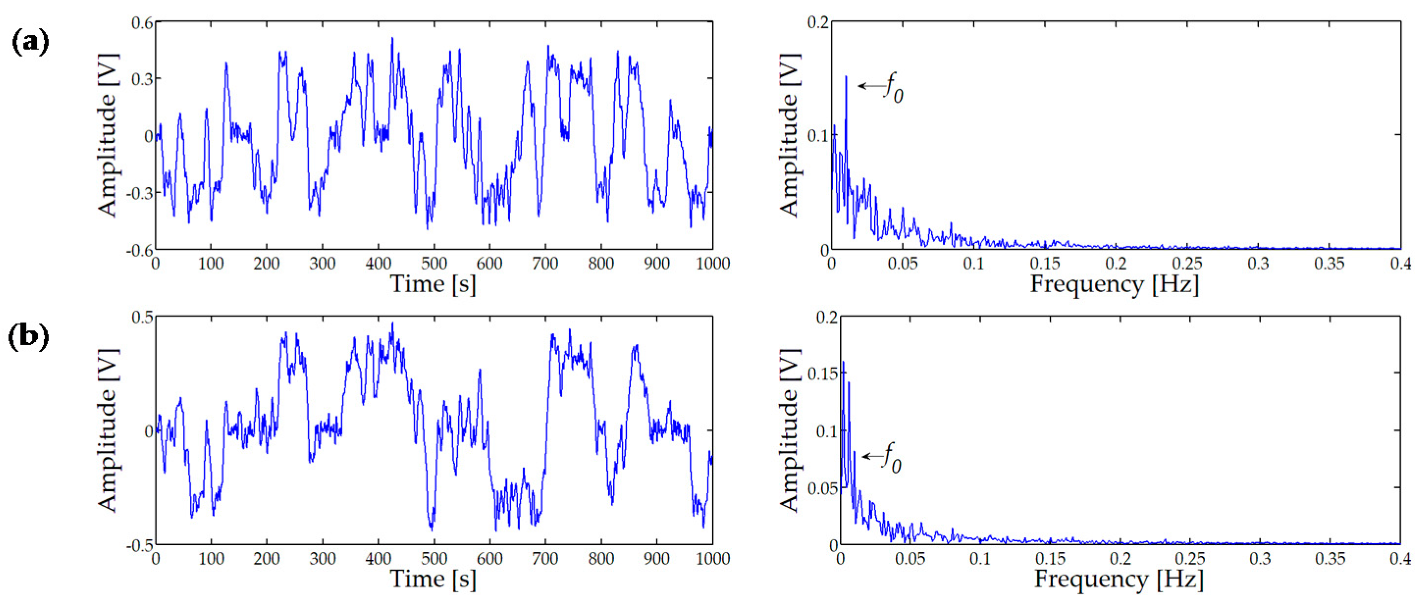
Then, we explore the effect of damping ratio
k on the STSR performance. In the same way, we use the signal of Equation (8) as the input of STSR to analyze the influence of
k on the output signal. We cannot see the 0.01 Hz from
Figure 5b, when
D = 0.3,
a = 0.4,
b = 2.7,
V = 11,
r = 39,
c = 20, and
k = 0.47. We can fix parameters
a,
b,
V,
r,
c, and make
k = 0.5334, seeing 0.01Hz clearly from
Figure 6a that shows the result of STSR. When the damping ratio
k is increased to 0.885, the time-domain waveform and amplitude spectrum of the output signal are as shown in
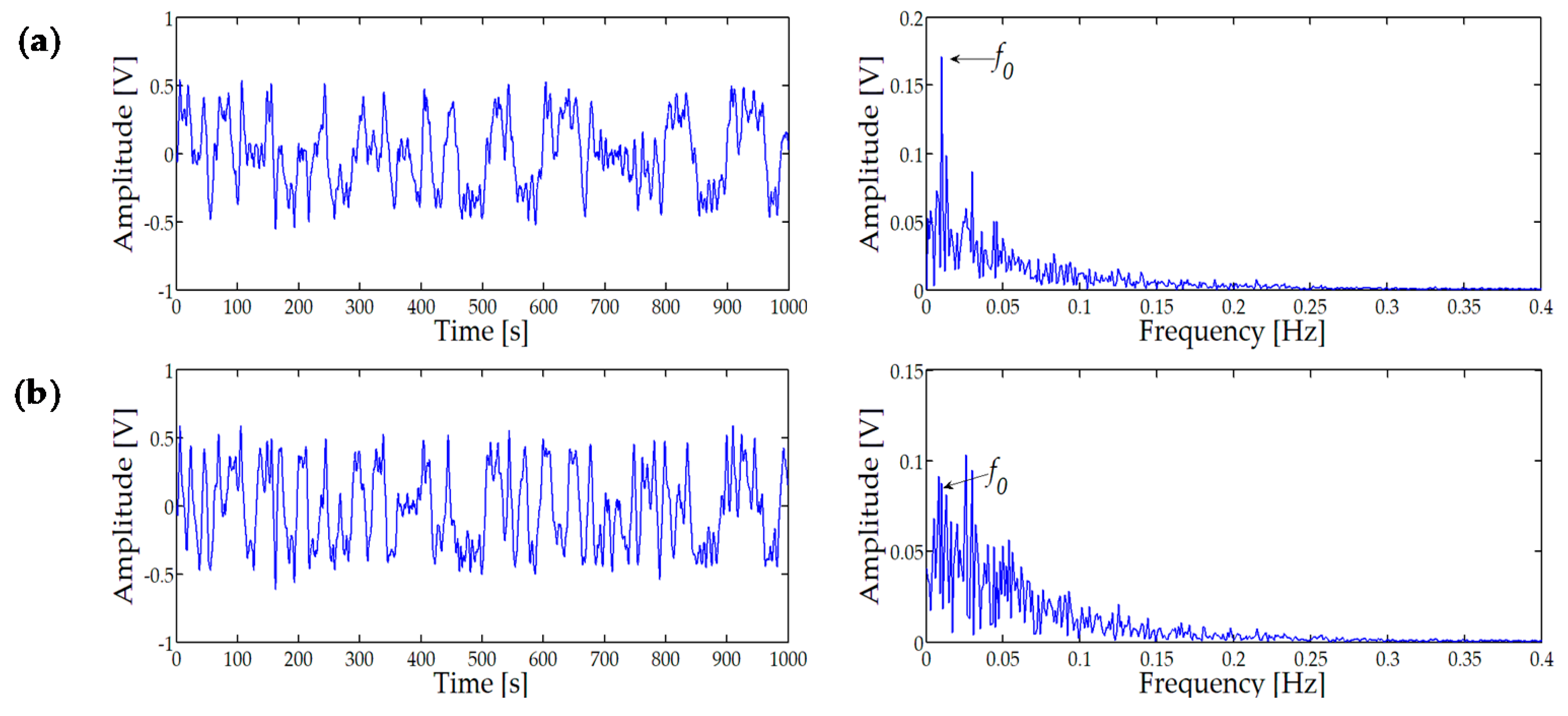
Figure 6b. The 0.01 Hz cannot be discerned from the amplitude spectrum. The signal with noise intensity
D = 0.8 is analyzed to fully explain the effect of damping ratio
k on STSR. When the damping ratio
k = 0.47, the characteristic frequency of 0.01 Hz cannot be recognized from the amplitude spectrum of
Figure 5d.
Figure 7a displays the time-domain waveform and amplitude spectrum of STSR output signal when
k is decreased to 0.375. It can be observed that 0.01 Hz is very obvious in the whole amplitude spectrum, although there are many frequency components in the whole spectrum. Continue to reduce the damping ratio
k to 0.235, and the time-domain waveform and amplitude spectrum are as shown in
Figure 7b, from which the frequency of 0.01 Hz cannot be observed. Thus, the damping ratio
k affects the characteristics of the STSR system.
2.4. Procedure of Proposed Method
We can see the effect of noise intensity
D and damping ratio
k on STSR based on the above analysis. Since system parameters
a,
b,
V,
r, and
c are artificially selected, they are no longer analyzed. While the noise intensity
D has a certain influence on the output signal of STSR, it cannot be controlled. Thus, it can be understood that the system parameters
a,
b,
V,
r,
c, and the damping ratio
k affects the performance of the STSR. Due to the fault characteristic frequency of the bearing is far larger than 1 Hz, the frequency compression scale (
R) is introduced by the re-scaling frequency technique to satisfy the small parameter limitation in this paper. This paper uses the Seeker Optimization Algorithm (SOA) to optimize seven parameters synchronously [
29,
30]. Output SNR is often used to evaluate the performance of SR, which specifies the calculation as follows:
where
is a discrete signal.
where
f0 represents the frequency at the highest spectral peak and
fs is the sampling frequency of the signal. SNR can be defined as:
The specific procedure of the STSR method based on SOA can be expressed as follows:
- (1)
Signal preprocessing. The vibration signal is filtered by band-pass filter to eliminate some noise components. Hilbert transform is used to demodulate the filtered signal, in which the obtained signal is marked as S1. , . S is the input signal of STSR system.
- (2)
Parameter initialization. Setting population size, number of iterations, and range of parameters including a, b, V, R, c, k, and R.
- (3)
Calculate the objective function value of each location according to Equation (11).
- (4)
If the number of iterations reaches the set value, the process goes to step (5), otherwise it returns to step (3).
- (5)
The optimal record of output is the value of a, b, V, r, c, R, and k at the maximum SNR.
- (6)
Weak signal detection. The optimal parameters are substituted for the STSR system. Additionally, the pre-processed signal is used as the input signal of the STSR to obtain the output signal. Restore the signal amplitude and frequency scale to plot time-domain waveform and amplitude spectrum.
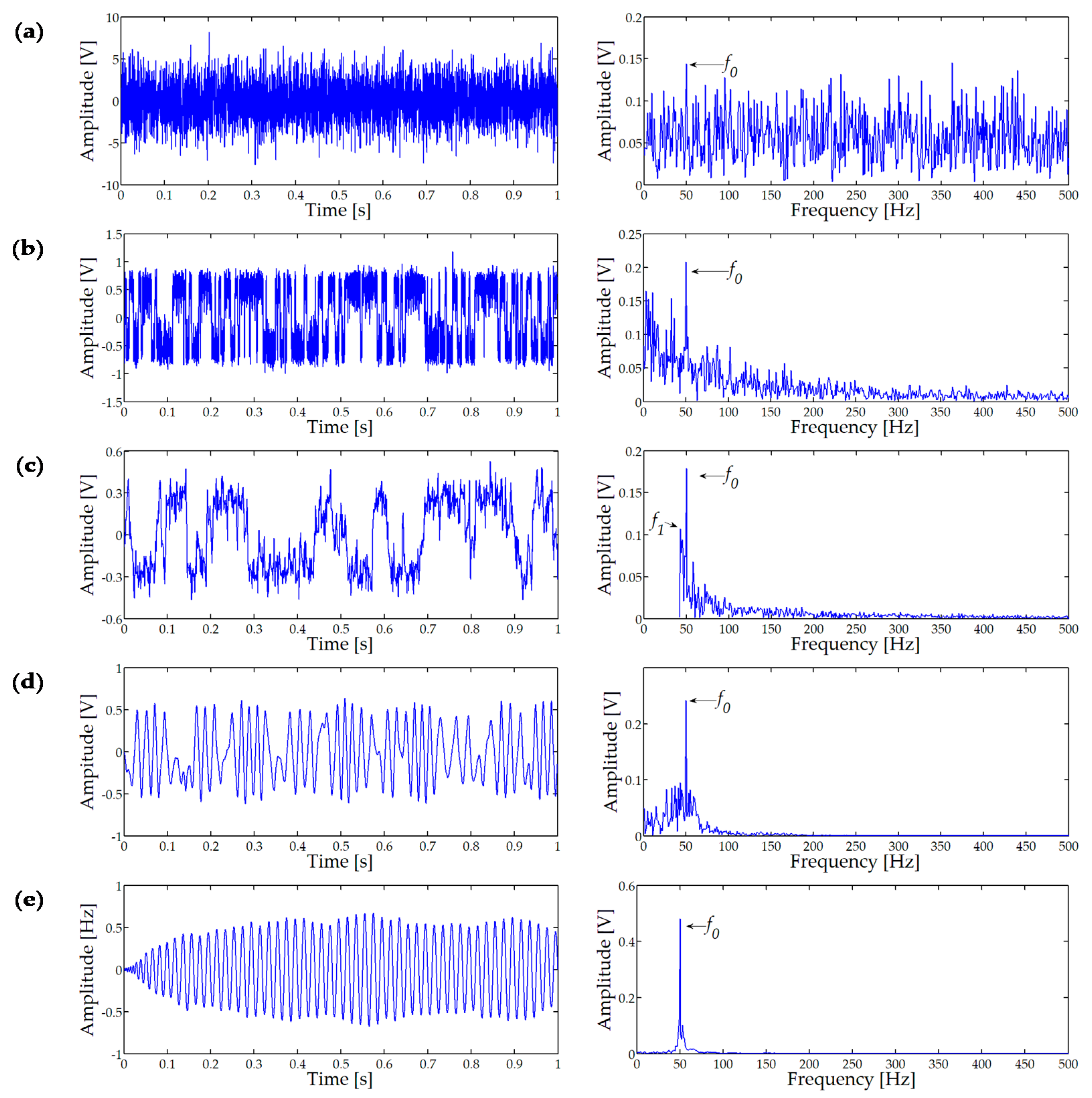
3. Simulation Analysis
The simulation analysis is used to prove the effectiveness of the proposed STSR method. The simulation signal is defined as:
where
A0 = 0.2,
f0 = 50 Hz,
n(
t) is Gaussian white noise, and the intensity is
D = 2.4.
The sampling frequency
fs = 5 kHz, and sampling number is 5000. Experimental environments are Intel (R) core (TM) i5-7400 (Beijing, China) CPU 3.00 GHz, 8 G RAM, Windows 10, and MATLAB R2018a. The time-domain waveform and amplitude spectrum of signal are shown in
Figure 8a. The periodicity of the signal cannot be seen from the time domain waveform and 50 Hz cannot be discovered from the amplitude spectrum. According to Equation (11), the SNR of the signal with noise is −29.82 dB. The optimal output result of CSR [
13] is shown in
Figure 8b where the parameters are
a = 19.72,
b = 7217.256,
R = 464.03, and SNR = −20.53 dB. While the SNR is improved, the noise energy is also enhanced. Additionally, the low-frequency components are amplified.
Figure 8c shows the optimal output of the frequency-shifted and re-scaling SR [
11]. The cutoff frequency of the high-pass filter is set to 35 Hz, the modulation frequency is 40 Hz, and the target frequency is 10 Hz in this method with optimization results are
a = 1.86,
b = 4794.73,
R = 140.97, and SNR = −13.38 dB. It can be seen that the SNR of frequency-shifted and re-scaling SR is further improved than CSR, but the interference frequency
f1 of the filter can be seen from
Figure 8c. Additionally, the artificially set cutoff frequency of the filter may also affect the stochastic resonance system performance.
The USSSR [
23] is used to deal with simulation signal and the result shows in
Figure 8d where optimization parameters are
a = 2.343,
b = 10,431.066,
k = 0.13,
R = 131.44, and SNR = −11.49 dB. It can be seen that the characteristic frequency is significantly enhanced. The simulation signal further demonstrates that the filtering performance of the second-order SR system is better than that of the first-order SR system. The same signal is analyzed by the proposed STSR method, and the result is displayed in
Figure 8e. Obvious period components can be found from the time domain waveform, and the characteristic frequency
f0 can be clearly seen from the amplitude spectrum, while other frequencies are almost nonexistent. The optimization parameters are
a = 10.23,
b = 17186.47,
k = 0.179,
V = 31.56,
r = 7.254,
c = 6.5,
R = 60.508, and SNR = −6.53 dB at this time. Therefore, the proposed method can obtain larger output SNR and better filtering performance than traditional SR methods for detecting weak signals.
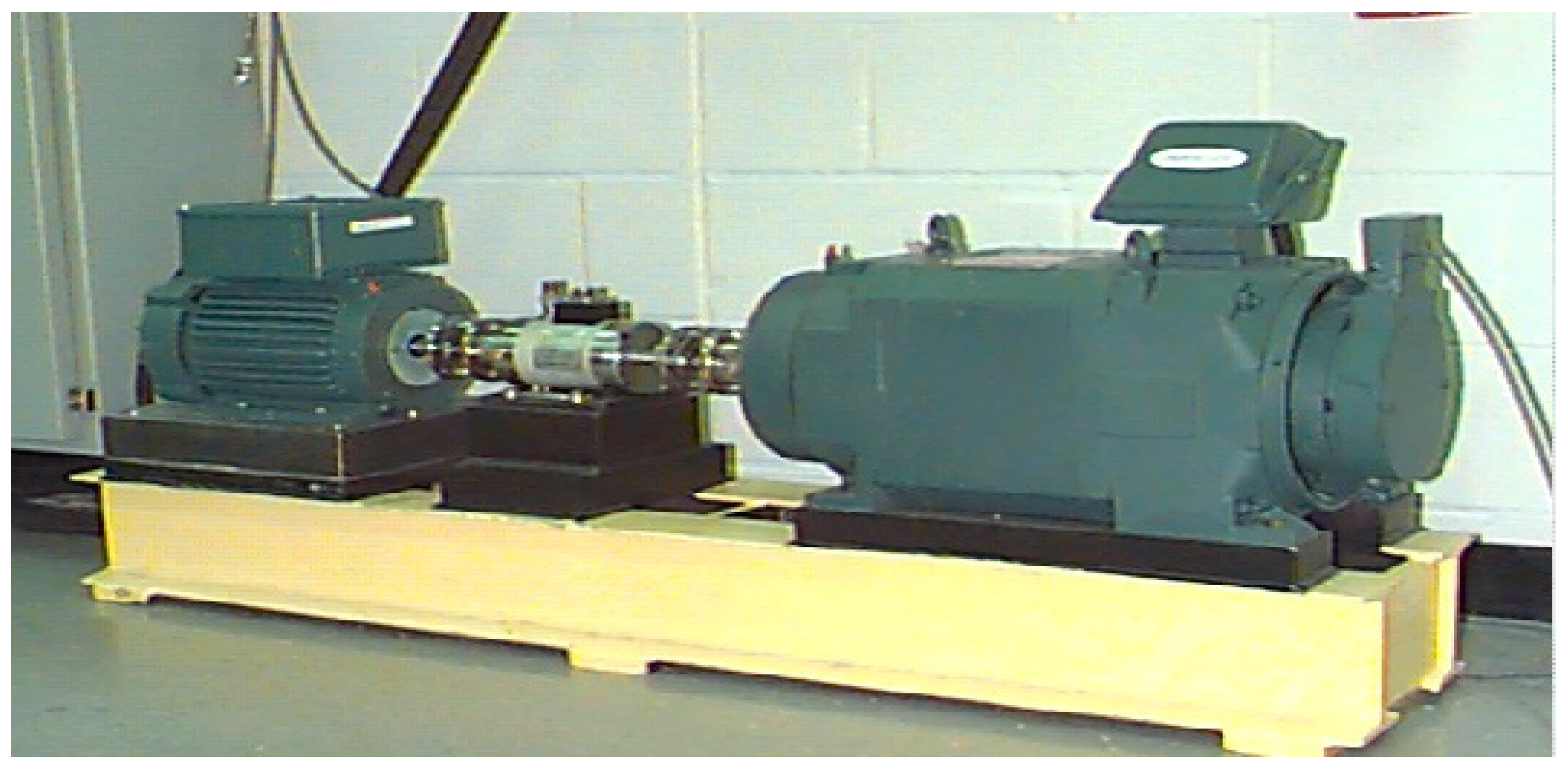
4. Experimental Verification and Analysis
To confirm the effectiveness of proposed method in practical engineering applications, a set of vibration signals are analyzed. Meanwhile, to indicate the better STSR method, the same signals are processed using the CSR method and USSSR method. The experimental data comes from the Case Western Reserve University (CWRU) Bearing Center website [
31,
32,
33,
34]. The experimental test platform is shown in
Figure 9. The bearing is the deep groove ball bearing with the type of 6205-2RS JEM SKF, where a physical dimension is shown in
Table 1. The sampling frequency
fs is 12 kHz and sampling points are 4096. The fault characteristic frequencies for outer ring and inner ring are expressed by
fBPFI and
fBFO, respectively, that can be theoretically calculated as follows:
where
n is the number of rolling elements,
fr is rotating frequency of shaft,
d is ball diameter,
D is pitch diameter, and
is the contact angle, respectively.
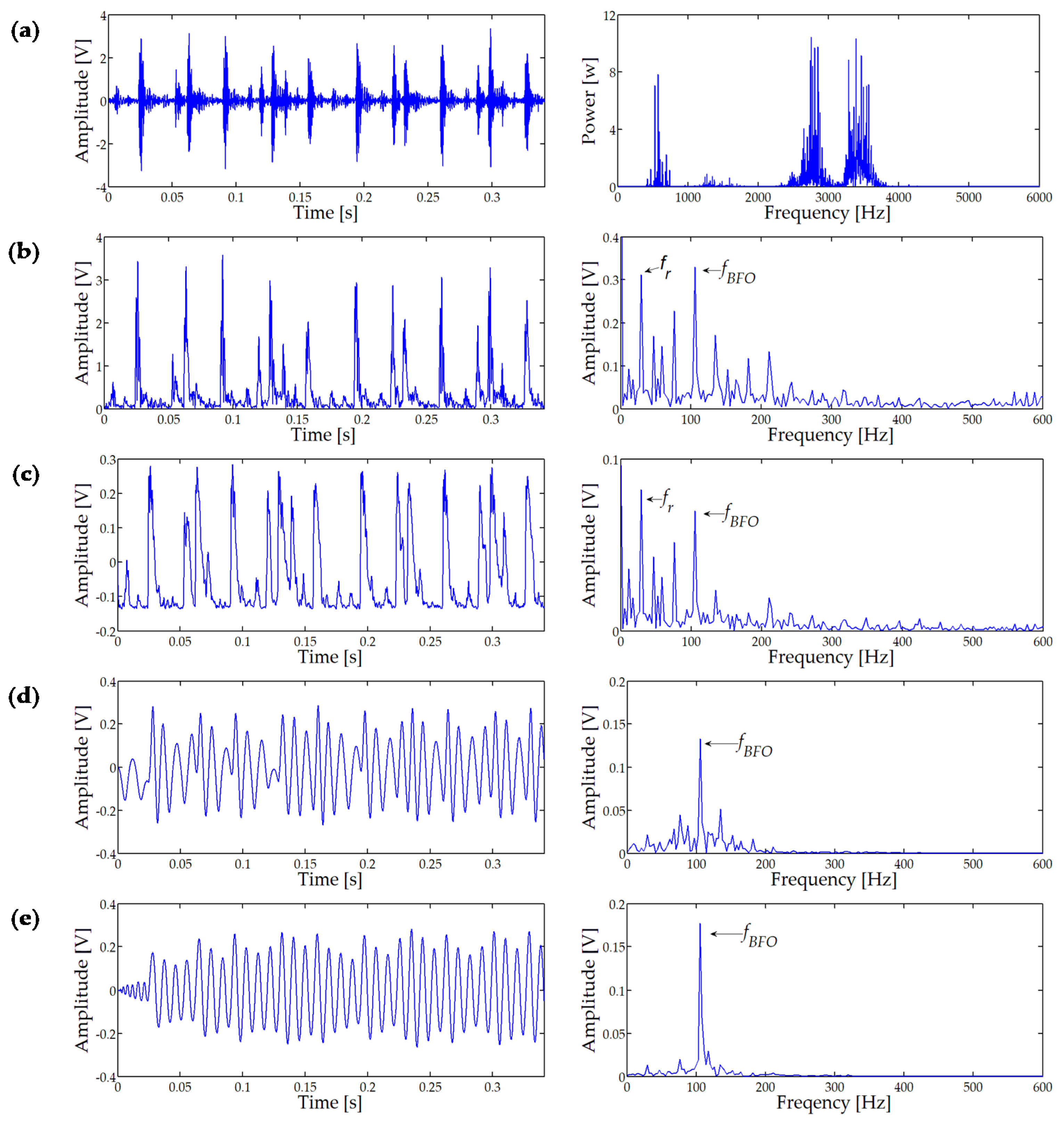
4.1. Outer Race Fault Signal Detection
In the first case, the bearing signal with an outer fault is tested to verify the performance of STSR. According to Equation (13), the fault characteristic frequencies of outer ring is theoretically
fBFO = 105.9 Hz with an approximate rotating speed of 1772 r/min.
Figure 10a shows the original vibration signal wave and its power spectrum. It is found that the periodic component cannot be seen from time domain and the low frequency signal is modulated to the high frequency band. Firstly, the fault signal is filtered using the band-pass filter at 2000–4000 Hz. Then, Hilbert transform demodulated the filtered signal. Additionally, the enveloped signal and its amplitude spectrum are displayed in
Figure 10b. While the characteristic frequency
fBFO can be seen from the amplitude spectrum, and the noise is still obvious in spectrum with output SNR = −15.02 dB.
The output result of CSR is shown in
Figure 10c, where the parameters are
a = 0.002,
b = 5656,
R = 579, and output SNR = −13.21 dB. We can see that the energy of the high frequency is significantly reduced, while the energy of
fBFO is amplified and the energy of the rotating frequency is greatly amplified. Then, the enveloped signal is analyzed by the USSSR method. Additionally, the results are exhibited in
Figure 10d where
a = 0.46,
b = 11471,
R = 221.5,
k = 0.434, and output SNR = −8.357 dB. Finally, the proposed STSR method deals with the same signal and
Figure 10e display the time domain waveform and amplitude spectrum of the output signal. The fault characteristic frequency
fBFO can be clearly seen in the whole spectrum diagram where
a = 8.282,
b = 14244.13,
k = 0.434,
V = 35.725,
r = 15.451,
c = 14.328,
R = 143.929, and the output SNR = −5.09 dB.
The analysis results of the bearing outer ring fault signal shows that the filtering performance of STSR is significantly better than CSR and USSSR. In other words, it indicates the validity and superiority of the proposed STSR method.
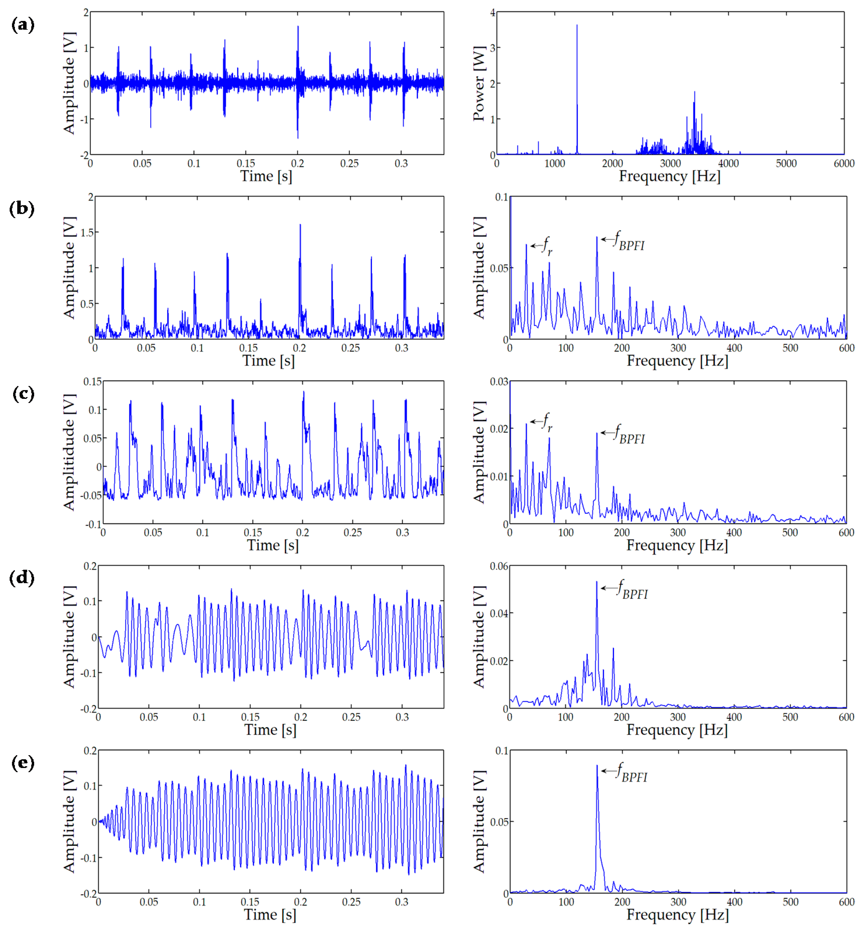
4.2. Inner Race Fault Signal Detection
To further verify the reliability of proposed STSR method, the inner race fault signal is analyzed. According to Equation (14), the characteristic frequency of inner race is theoretically
fBPFI = 156.1 Hz with approximate rotating speed of 1730 r/min.
Figure 11a shows the time waveform of inner race fault and its power spectrum. It is hard to see the fault characteristic frequency from
Figure 11a, due to the strong noise. The origin vibration signal was filtered by a band-pass filter in a bandwidth of 2000–4000 Hz and demodulated by Hilbert transform, then we got the envelop signal which is displayed in
Figure 11b with output SNR = −17.53 dB. The CSR method was employed to test the envelop signal and the results are shown in
Figure 11c. It can be observed that most of the high frequency noises are suppressed, but low frequency noises are enhanced where
a = 0.0015,
b = 5235.68,
R = 672.536, and output SNR = −15.511 dB. Output results of the USSSR system are shown in
Figure 11d with parameters of
a = 0.908,
b = 12476.8,
k = 0.222, and
R = 304.395. It can be seen the
fBPFI clearly in the amplitude spectrum and the output SNR is improved to −10.42 dB. The proposed STSR method is utilized to analyze the same signal. The optimal diagnosis result is displayed in
Figure 11e where
a = 7.534,
b = 9801.33,
c = 10.97,
V = 34.07,
R = 206.5,
r = 12.71,
k = 0.222, and the output SNR = −6.23 dB. It can be seen that fault characteristic frequency
fBPFI is prominent in the whole spectrum, which also demonstrate the effectiveness of the proposed STSR method than the traditional SR methods in bearing fault diagnosis.
4.3. Discussion and Anlysis
Table 2 lists SNRs using different SR methods based on the above analysis. The comparison results show that the SNR of fault signals processed by STSR are higher than those of other methods. It also proves that STSR has better performance in the extraction of weak signals.
The SR acts like a specific filter. The second-order SR system [
23] provides a secondary filtering effect, while the first-order SR system corresponds to a filtering effect and it can be observed that USSSR output SNRs are higher than the CSR from
Table 2. Thus, this paper explores second-order SR systems. Additionally, the tristable SR method [
17] has a better effect than the classical bistable SR method in weak signal detection using first-order SR system. Therefore, the STSR method is proposed in this paper. The experimental results show that the proposed STSR method obtains higher than the CSR method and USSSR method and has a better filtering effect for weak signals.
The SR theory is developed with the regime of small parameter limitation (the input signal of SR model amplitude and frequency are less than 1); therefore, the rescaling frequency is utilized to detect bearing fault signals. The system parameters are crucial in determining the SR output. Hence, this work adjusts parameters synchronously using SOA. While STSR improve output signals with less interference components, SNR is the criterion to select system parameters. SNR criterion requires the precise frequency of detecting signal, the criterion establishment of SR is a key research direction in the future.


