Article

The Solutions of Non-Integer Order Burgers’ Fluid Flowing through a Round Channel with Semi Analytical Technique

1
Department of Mathematics, Government College University, Faisalabad, Punjab 38000, Pakistan
2
Fundamental and Applied Science Department, Universiti Teknologi Petronas, 32610 Perak, Malaysia
3
Faculty of Mathematics and Statistics, Ton Duc Thang University, Ho Chi Minh City 72915, Vietnam
4
Department of Mathematics, University of Management and Technology Lahore, Punjab 54770, Pakistan
5
Department of Mathematics, College of Arts and Science, Prince Sattam bin Abdulaziz University, Wadi Al-Dawaser 11991, Saudi Arabia
*
Author to whom correspondence should be addressed.
Symmetry 2019, 11(8), 962; https://doi.org/10.3390/sym11080962
Submission received: 4 April 2019 / Revised: 5 May 2019 / Accepted: 6 May 2019 / Published: 1 August 2019
(This article belongs to the Special Issue Aero/Hydrodynamics and Symmetry)

Abstract

:
The solutions for velocity and stress are derived by using the methods of Laplace transformation and Modified Bessel’s equation for the rotational flow of Burgers’ fluid flowing through an unbounded round channel. Initially, supposed that the fluid is not moving with t = 0 and afterward fluid flow is because of the circular motion of the around channel with velocity Ω R t p with time positively grater than zero. At the point of complicated expressions of results, the inverse Laplace transform is alternately calculated by “Stehfest’s algorithm” and “MATHCAD” numerically. The numerically obtained solutions in the terms of the Modified Bessel’s equations of first and second kind, are satisfying all the imposed conditions of given mathematical model. The impact of the various physical and fractional parameters are also indeed and so presented by graphical demonstrations.

1. Introduction

Fluids can be divided into two types i.e., Newtonian and non-Newtonian fluid. The Newtonian fluids are simple and ideal. In real life there is no exitance of Newtonian fluids but water and air consider as Newtonian fluid. However, the non-Newtonian fluids are complicated and cannot be solved easily. The fluid motion within a cylinder has a wide application in the field of physics, engineering and specially in the food industry. In (1923), Taylor presented the results of stability of fluid in rotating cylinders [1]. Stephen Childress, in 2009 talked about the lift and drag in ideal fluids in two-dimensional, Stoke’s flow and gas dynamics [2]. Waters and King [3] discussed the Oldroyd-B fluid in a circular tube by taking Poiseuille flow into account. The investigation of basic unsteady pipe flow and viscoelastic upper-convected Maxwell fluid in uniform circular cross section, is available in [4]. They used the Fourier Bessel series to obtain the closed form solutions. The exact solutions of different fluids in circular cylinders (may be finite and infinite) can be obtained by applying the Laplace transformation on the system. There has been published a number of papers on this idea.
The action of circular cylinder and pressure gradient for both translational and rotational flows for viscoelastic fluids discussed in [5]. Fox and Macdonald [6] focussed on differential analysis of one dimensional and steady state flow of incompressible and non viscous fluid. He also discussed the flow of fluid through pipes and channels. Fetecau [7] worked on unidirectional unsteady flow through an infinite pipe for Oldroyd-B fluids. For analytical solutions, an expansion theorem of Steklov is used with a no slip condition. The viscoelastic fluids have many exertions in various fields of industry, also in bio engineering. Ting [8] and Srivastava [9] find out the analytical solutions of non-Newtonian fluids for second grade and Maxwell fluids respectively. Sherief et al. [10] considered an infinitely magnetic insulating circular cylinder for the steady one-dimensional flow of an incompressible MHD fluid. The slip boundary conditions are applied on velocity and they calculated the results for the micro rotation, ratio of flow and skin coefficients.
The Helical flow is the composition of translation and rotational motion, is applicable in vascular hydrodynamics and biomedical engineering. Many papers have been published on this type of flow. The general solutions of some helical flow corresponding to the second grade fluid are seems in [11]. The analytic solutions of same fluid for unsteady flow has been derived by Hayat et al. [12]. In rotating circular cylinder, Fetecau [13] obtained the analytical solutions for the helical flow of Oldroyd-B fluid. In the same domain, the solutions of Maxwell and second grade fluids are available in [14,15].
Fractional calculus plays a very important rule in the field of fluid mechanics. Podlubny [16] discussed the differential equations of fractional model. The elements of fractional model defines viscoelastic fluids of special kind. Now a days, such models frequently [17,18] commonly encounter in our daily lives. The analytical solutions of generalized second grade fluids are available in [19]. Exact solutions of generalized Burgers’ fluid in annulus of circular cylinders and helical flow of Burgers’ fluid, in terms of fractional derivatives, are found in [20,21] respectively. Whereas the analysis of velocity and stress field, vortex sheet of same fluid by considering the fractional anomalous diffusion by Xu et al. [22]. Song and Jiang [23] studied the five parametric constitutive equations with fractional derivatives of linear viscoelastic Jeffreys model. For the applications, they consider the Sesbania gel and Xanthan gum and get the satisfactory results. Tan et al. [24] and Xu et al. [25] applied a fractional derivative model to Maxwell and generalized second grade fluids between two parallel plates. Abdullah et al. [26] considered the fractional Maxwell fluid in a boundless circular pipe with velocity f t . To obtained the solutions for velocity and shear stress they applied the Laplace transformation and modified Bessel equation. To find out numerically inverse Laplace transformation MATLAB is used by them.
In this article, the solutions for Burgers’ fluid in rotating pipe like domain are determined. Here, a Laplace transformation technique was used to study fluid motion in a circular domain. The variable of time is removed with the help of a Laplace transform and modified Bessel functions to convert the complex equations into simple algebraic equations. The derived results are complicated so that inverse Laplace transformation were difficult to apply. So “Stehfest’s algorithm” [27] and “MATHCAD” software was used to find the numerical solutions for the Burgers’ fluid in circular domain. Graphs were drawn to elaborate the influences of fluids on velocity against different parameters. The results and discussions of all parameters are given at the end that shows the consistency in obtained results.

2. Governing Equations

Here, the formulation of velocity V and the extra-stress S for the fluid under consideration are as [28]
V = V ( r , t ) = F ( r , t ) e θ , S = S ( r , t ) ,
where e θ is the unit vector of the cylindrical coordinates system and F ( r , t ) is the component of velocity along e θ . The initial conditions for the fluid at rest position are, as in [28];
V ( r , 0 ) = 0 , S ( r , 0 ) = 0 .
The governing equations for the motion of Burgers’ fluid are [29]
1 + λ 1 t + λ 2 2 t 2 F t = ν 1 + λ 3 t 2 r 2 + 1 r r 1 r 2 F ( r , t ) ,
1 + λ 1 t + λ 2 2 t 2 Q ( r , t ) = μ 1 + λ 3 t r 1 r F ( r , t ) ,
where μ is the coefficient of viscosity, ν = μ / ρ is kinematic viscosity, ρ is constant density of the fluid, λ i ( i = 1 , 2 , 3 ) new material constants and Q ( r , t ) = S r θ ( r , t ) 0 shear stress. By altering the inner time derivatives with the fractional derivatives in Equations (3) and (4), the governing equations for the fractional derivative of Burgers’ fluid (FBF) can be obtained as
1 + λ 1 α D t α + λ 2 2 α D t 2 α F ( r , t ) t = ν 1 + λ 3 β D t β 2 r 2 + 1 r r 1 r 2 F ( r , t ) ,
1 + λ 1 α D t α + λ 2 2 α D t 2 α Q ( r , t ) = μ 1 + λ 3 β D t β r 1 r F ( r , t ) ,
where α and β are the fractional parameters such as 0 α β 1 . The Caputo fractional derivative is defined as [16,18]
D t α f ( t ) = 1 Γ ( 1 α ) d d t 0 t f ( τ ) ( t τ ) α d τ , 0 α < 1 ; d d t f ( t ) , α = 1 ,
where Γ ( · ) is the gamma function. When α , β 1 , Equations (5) and (6) reduce to Equations (3) and (4), because D t 1 f = d f d t .

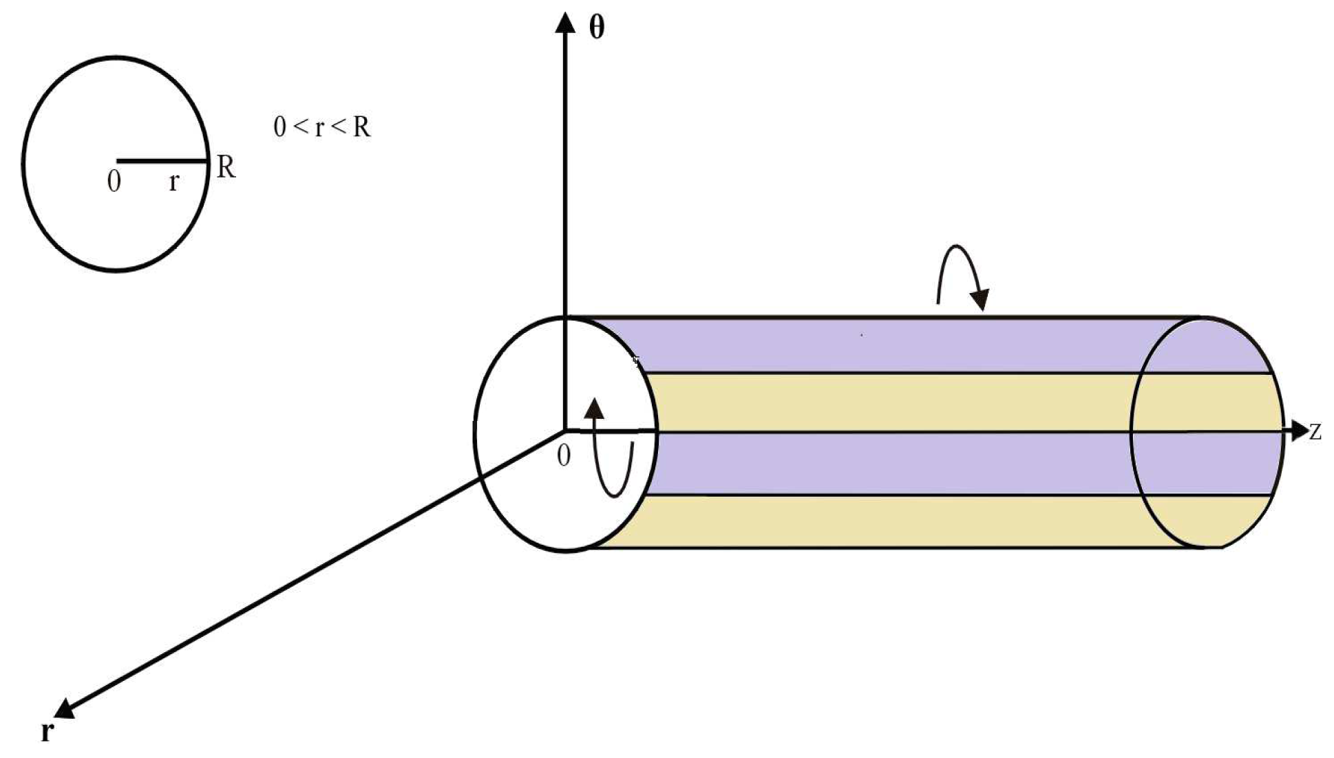
3. Imposing Condition and Geometry

Initially, (when t = 0 ) the FBF is at rest in an infinite circular pipe with radius R ( > 0 ) as shown in Figure 1. After time t = 0 + , the pipe suddenly starts to rotate about its Z-axis having the angular velocity Ω t p . According to mathematical situation, appropriate initial and boundary conditions are
F ( r , 0 ) = F ( r , 0 ) t = 0 , τ ( r , 0 ) = 0 ; r [ 0 , R ] ,
F ( R , t ) = R Ω t p ; t > 0 , p N , p > 0 ,
where Ω denotes the angular constant and N is the set of natural numbers.

3.1. Velocity Field Due to Rotating Circular Pipe

By applying the Laplace transform to Equations (5) and (9),
2 F ¯ ( r , s ) r 2 + 1 r F ¯ ( r , s ) r 1 r 2 + a ( s ) F ¯ ( r , s ) = 0 ,
and
F ¯ ( R , s ) = R Ω p ! s p + 1 ,
where
a ( s ) = s ( 1 + λ 1 α s α + λ 2 2 α s 2 α ) ν ( 1 + λ 3 β s β ) .
Also F ¯ ( r , s ) and F ¯ ( R , s ) are the Laplace transforms of the functions F ( r , t ) and F ( R , t ) respectively. By applying the variable transformation z = r a ( s ) in Equation (10)
z 2 2 F ¯ r 2 + z F ¯ r ( 1 2 + z 2 ) F ¯ = 0 .
The above Equation (12) is the modified Bessel equation of order 1. So, the general solution of this equation is given by the successive equation
F ¯ ( z , s ) = C 1 I 1 ( z ) + C 2 K 1 ( z ) ,
where C 1 and C 2 are constants and I 1 , K 1 are the modified Bessel functions of first and second kind of order 1. For a finite solution at r = 0 ( z = 0 ) , the constant C 2 should be zero i.e., C 2 = 0 . So, Equation (13) implies
F ¯ ( z , s ) = C 1 I 1 ( z ) .
The value of C 1 is calculated from Equation (14) by taking Equation (11) into account
C 1 = Ω R p ! s p + 1 I 1 ( R a ( s ) ) .
Therefore the Equation (14) implies
F ¯ ( r , s ) = Ω R p ! s p + 1 × I 1 ( r a ) I 1 ( R a ) .
The solution in Equation (16) is in the complex form of the first and second kind of Bessel functions. Normally, it is difficult to find out the solution of such complex expressions with an ordinary inverse Laplace transformation. However, an alternately inverse Laplace of Equation (16) was numerically calculated by using the “Stehfest’s algorithm” [27]
f n ( x ) = l n ( 2 ) x 1 i = 1 2 n a i ( n ) F ( i ln ( 2 ) x 1 ) , n 1 , x > 0 ,
where a i ( n ) are coefficients defined as follows
a i ( n ) = ( 1 ) n + i n ! s = [ ( i + 1 ) 2 ] m i n ( i , n ) s n + 1 n C s 2 s C s s C i s , n 1 , 1 i 2 n ,
and “MATHCAD” software.

3.2. Shear Stress Due to Rotating Circular Cylinder

By taking the Laplace transform of Equation (6)
Q ¯ ( r , s ) = b ( s ) F ¯ ( r , s ) r 1 r F ¯ ( r , s ) ,
where
b ( s ) = μ ( 1 + λ 3 β s β ) ( 1 + λ 1 α s α + λ 2 2 α s 2 α ) .
Putting Equation (16) into (17) and after taking the few steps of simplification,
Q ¯ ( r , s ) = b s p + 1 × p ! Ω R I 1 ( R a ) a I 0 ( r a ) 2 r I 1 ( r a ) .
Again it is in a complicated form. So “Gaver Stehfest’s algorithm” and “MATHCAD” software were used for the inverse Laplace transformation of the result given in Equation (20).

4. Results and Discussions

In this article, the main goal is to establish the numerical technique to develop the solutions of the Burgers’ fluid for the rotational flow of Burgers’ fluid within cylindrical domain. The expressions of velocity and shear stress are found for an incompressible non-integer order model of the Burgers’ fluid in a circular pipe. The Laplace transformation is used to establish the solutions. As there are complicated expressions in Equations (16) and (20) with respect to the Laplace transformation, it was not easy to find out final results by using direct inverse Laplace on Equations (16) and (20). Although, “MATHCAD” is used along with the “Stehfest’s algorithm” instead of the inverse Laplace transformation to find out the numerical results. The numerical solutions for Oldroyd-B, Maxwell, second grade and Newtonian fluids are also derived with generalization of main results i.e., Equations (16) and (20). To determine the impact of physical parameters, the graphical illustrations are made. The behaviour of time on the velocity field and stress is shown in Figure 2 and Figure 3. These figures show that the influence of velocity and stress depending upon the parameters r , λ 1 , λ 2 , λ 3 , α , β , ν and μ . Figure 2 and Figure 3 show that the velocity and shear stress increase with respect to the increase in the dependent variable t with fixed values of other dependent parameters. Similarly, a clear increase in velocity and stress can also be seen in Figure 4 and Figure 5 for r with respect to the time variable t while fixing the other dependent parameters. It is also observed from Figure 4 that velocity has linear relation for r with respect to t.
Also, to uncover the aspects of other physical and fraction parameters on velocity and stress the graphs drawn and presented in Figure 6, Figure 7, Figure 8, Figure 9, Figure 10, Figure 11, Figure 12, Figure 13, Figure 14, Figure 15, Figure 16 and Figure 17. All the graphs for velocity and stress in Figure 6, Figure 7, Figure 8, Figure 9, Figure 10, Figure 11, Figure 12, Figure 13, Figure 14, Figure 15, Figure 16 and Figure 17 are plotted for concerned parameter against the change factor “time”. One can say that the fractional parameter α , relaxation parameters λ 1 and λ 2 have decreasing behaviour for velocity and stress with respect to t. This fact can be observed in Figure 6, Figure 7, Figure 8 and Figure 9, Figure 12 and Figure 13 respectively. Whereas, the velocity and stress are also increasing functions for the retardation parameter λ 3 , fractional parameter β , viscosity μ and ν with respect to time t as shown in Figure 10, Figure 11, Figure 14, Figure 15, Figure 16 and Figure 17. Figure 2, Figure 3, Figure 4, Figure 5, Figure 6, Figure 7, Figure 8, Figure 9, Figure 10, Figure 11, Figure 12, Figure 13, Figure 14, Figure 15, Figure 16 and Figure 17 make it possible to check the point to point variations, increment or decrement in two parameters (among which the graphs are made) for velocity and stress profile.
Finally, the comparison among the different generalized cases of Burgers’ fluid are made in Figure 18 for velocity function against time t. The results of these generalized cases are derived by the implementation of the “Stehfest’s algorithm” and “MATHCAD” to Equation (16). It is observed that the second grade fluids have more velocity as compared to other Newtonian and non-Newtonian fluid cases of this model while taking the same values of different dependent parameters and variation in time t. The Oldroyd-B fluid behaves as like the second grade fluid but have less velocity as compared to the second grade fluid’s velocity. Similarly, Figure 18 also shows the behaviour of velocity for Newtonian and Maxwell fluids. The Maxwell fluids have minimum velocity for this flow model with prescribed conditions among all the Newtonian and non-Newtonian cases. As a description it is clearing that in all the Figure 2, Figure 3, Figure 4, Figure 5, Figure 6, Figure 7, Figure 8, Figure 9, Figure 10, Figure 11, Figure 12, Figure 13, Figure 14, Figure 15, Figure 16, Figure 17 and Figure 18, the units of the material constants are SI units. The comparison of solutions that obtained from two different methods analytically [29,30] and numerically (derived from Equations (16) and (20)) are given in Table 1 and Table 2 for two different cases Maxwell and Newtonian fluids. These tables showing clearly that two different methods for the same problem have the same results. Which shows the consistency of our numerical technique and results for fractional model of Burgers’ fluid with already published literature [29,30].

5. Conclusions

The flow of incompressible Burgers’ fluid with leading equations in the terms of Caputo non-integer order derivatives is studied. The under consider flow is flowing through the circular channel of infinite length. The numerical solutions for velocity and stress has been drawn by utilizing the Laplace transformation along with the modified Bessel’s function. After the analysis of result following fruitful remarks are observed:
  • The ordinary fluid have less velocity as compared to fractional order derivative fluid models. This result can be verify from the graph of fractional parameter α available in Figure 12, which has decreasing altitude when the velocity is increasing.
  • The velocity of the fluid increases for Burgers’ fluid model as fluid becomes more thick in this model.
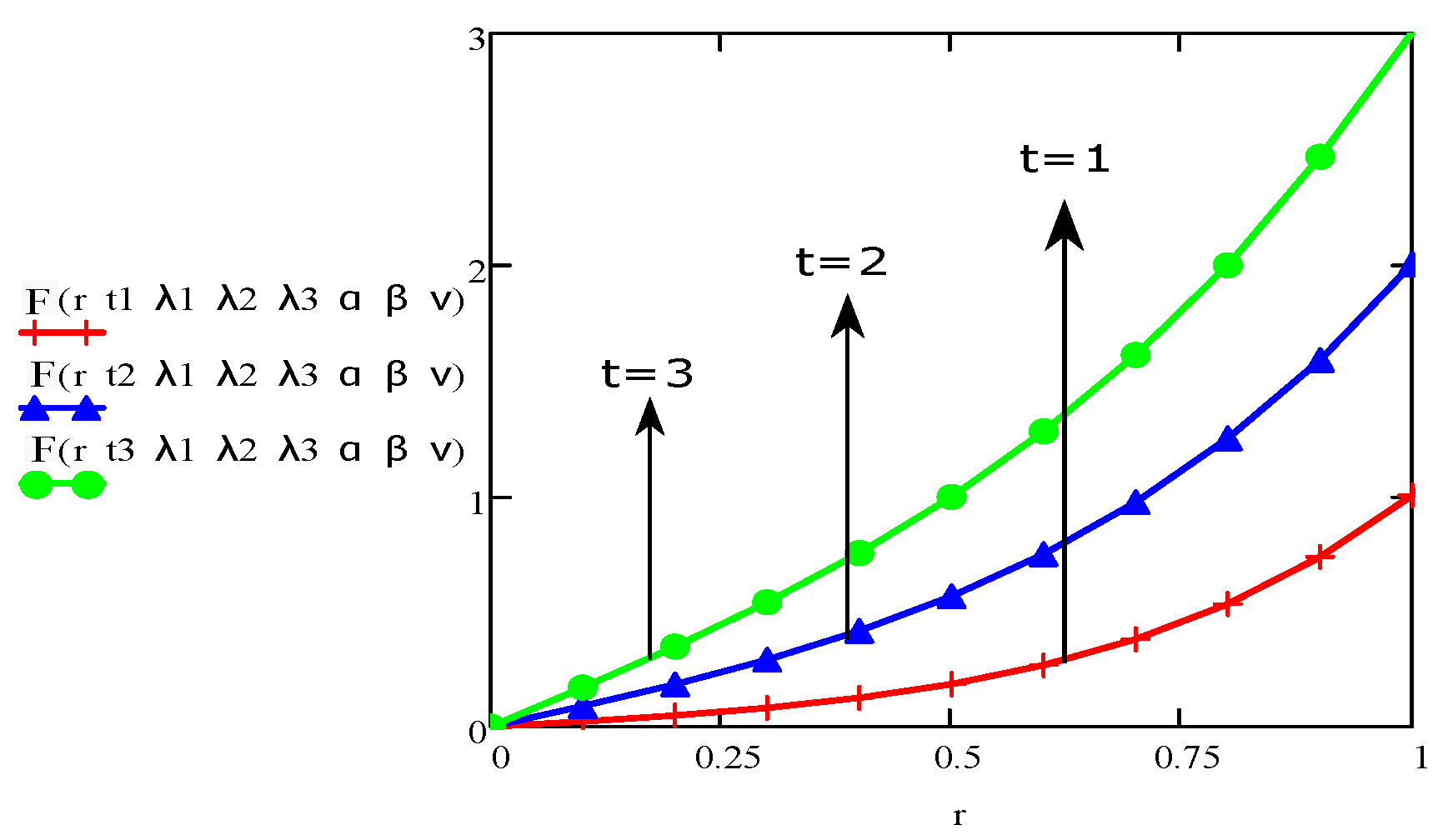
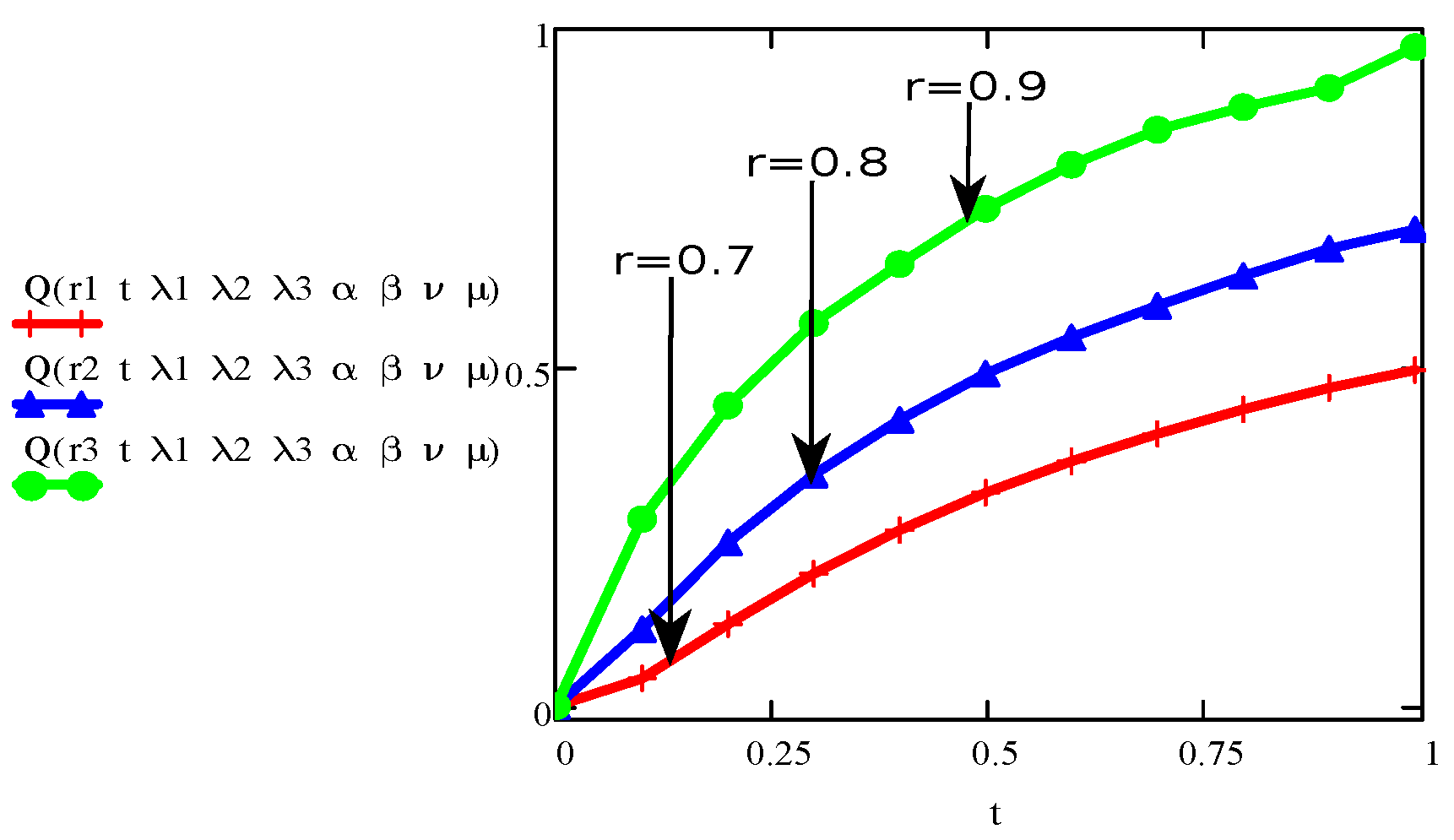
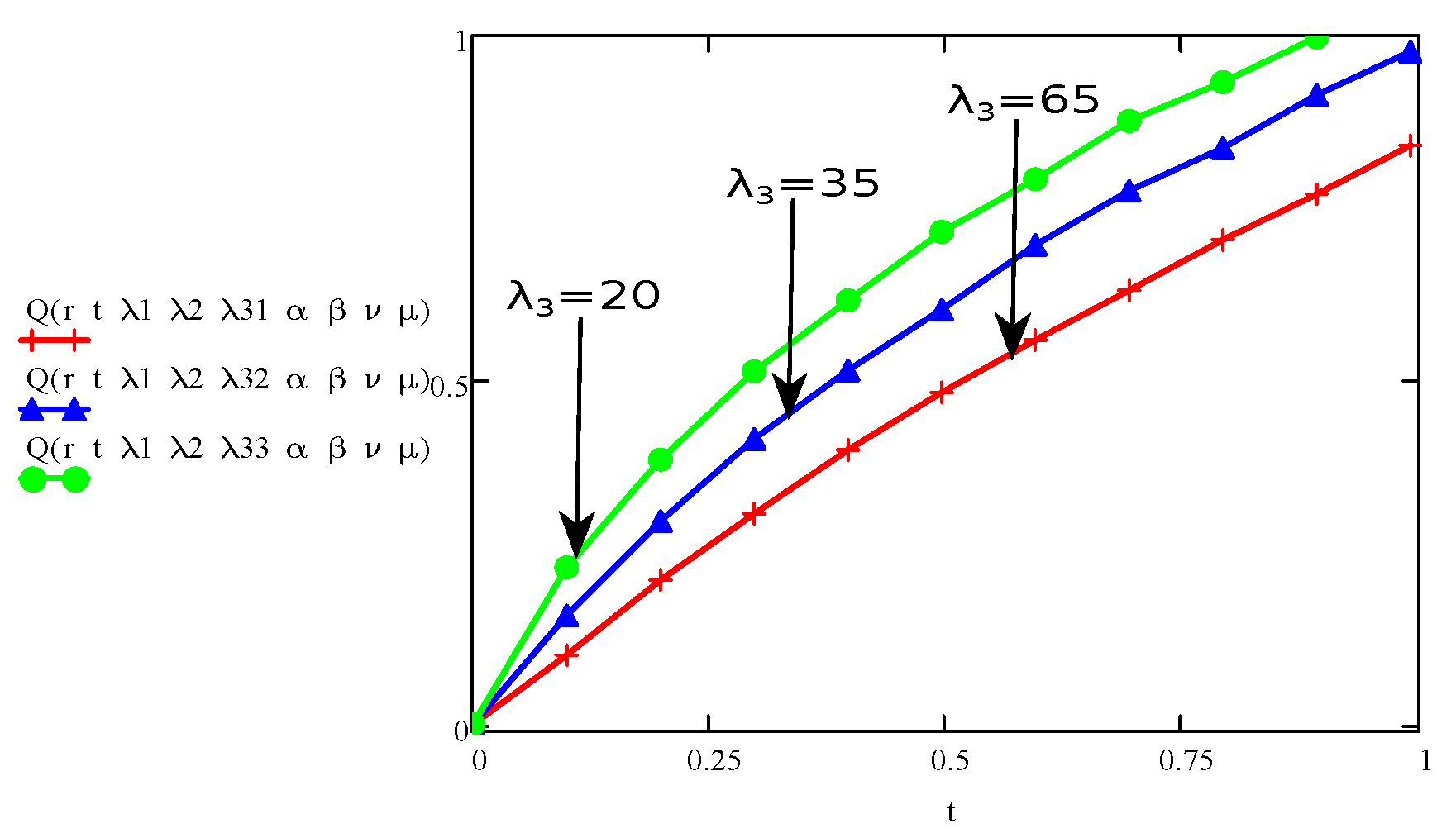
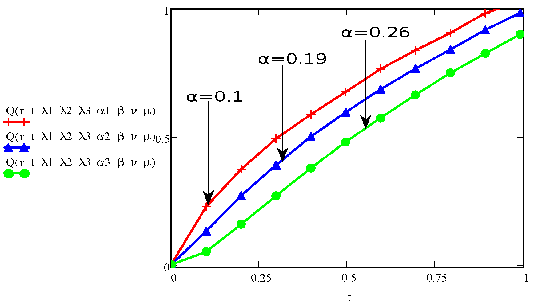
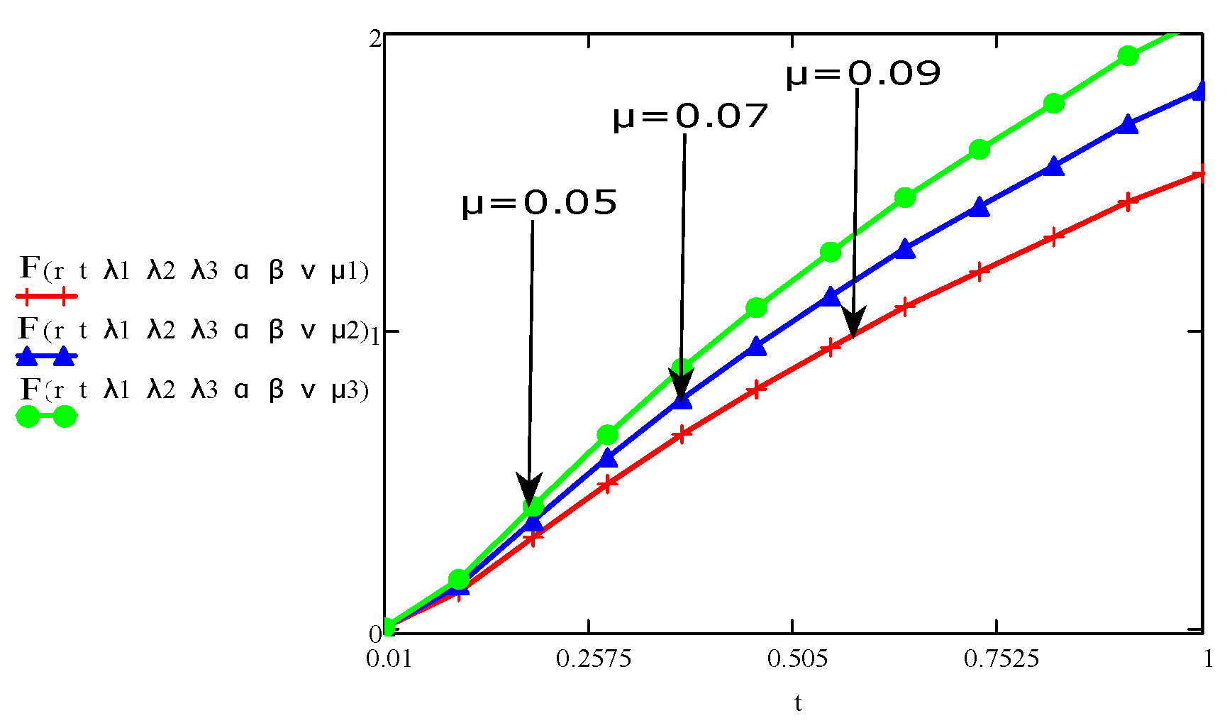
  • The graph of the parameters β , λ 3 , ν , t, r, and μ showed an increase/upward in behaviour with increase in velocity and stress function.
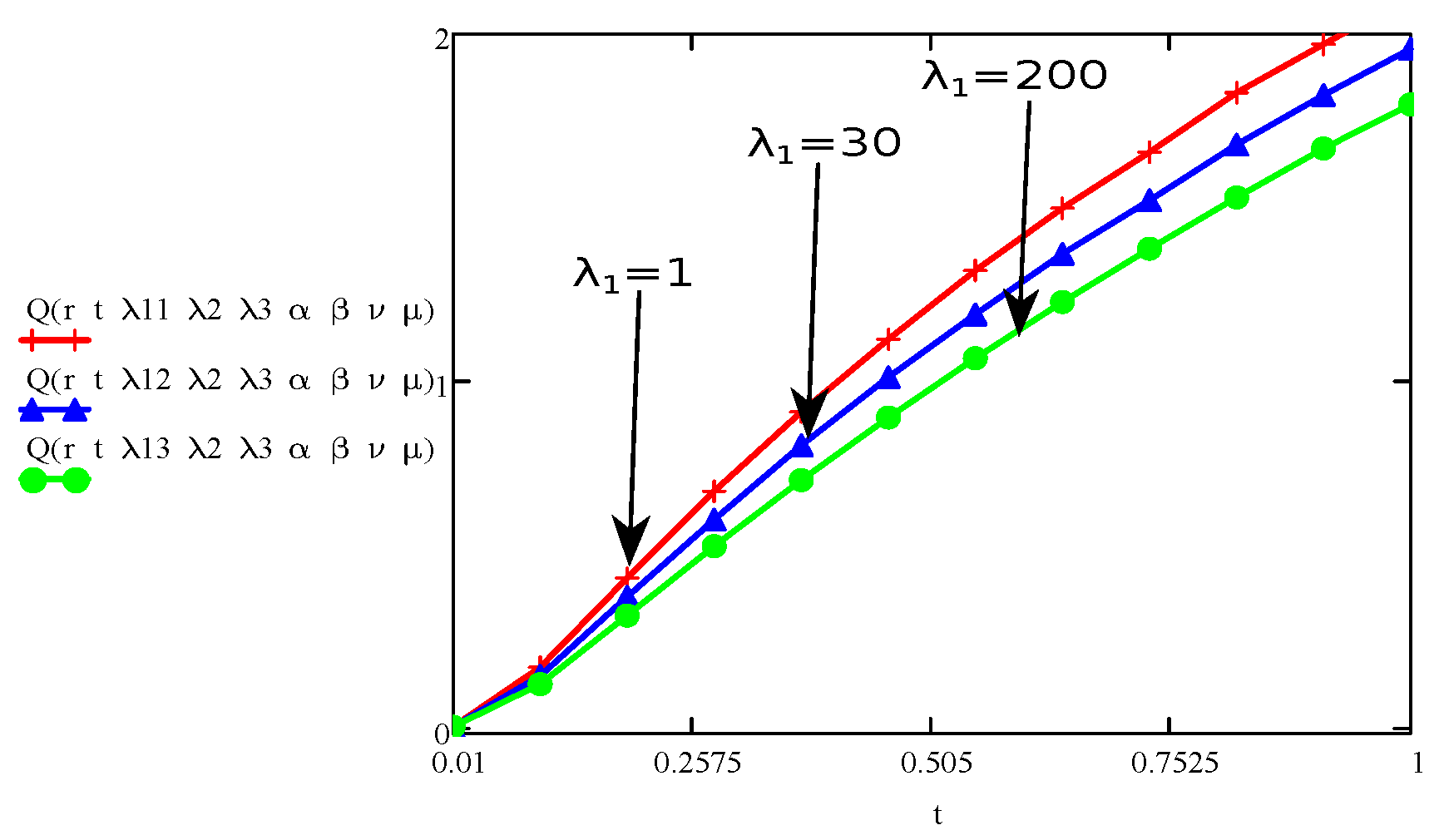
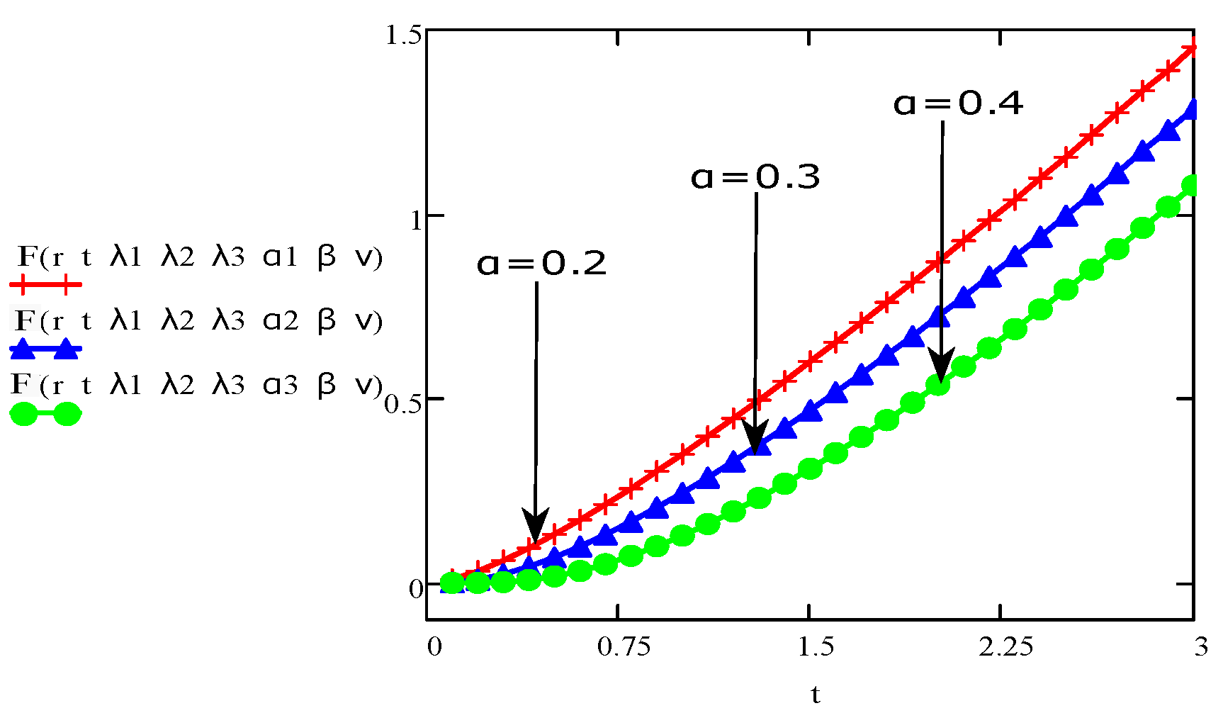
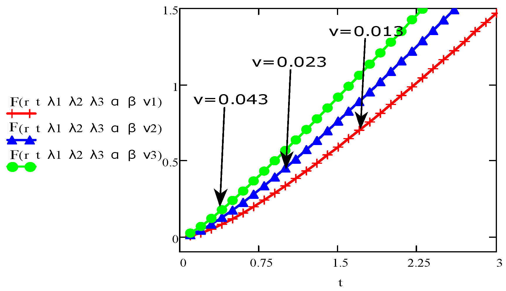
  • The parameters λ 1 , λ 2 and α are behaving opposite to the influence of velocity and shear stress.
  • The fractional Burgers’ fluid is flowing faster than the Maxwell and Newtonian fluids.
  • Our obtained solutions given in Equations (16) and (20) derived from “Stehfest’s inversion algorithm” and the exact solutions given in [29,30] are equivalent.
  • In future, authors will try to study the fluid motion by considering the effects of temperature and magnetic field.

Author Contributions

R.S. and M.I. made the mathematical model and mathematical calculation of the paper. M.A.I. and M.I. made the numerical results and graphs of the paper. I.K. wrote the manuscript. M.I. and R.S. checked the calculation and revised the manuscript. All authors read and approved the final manuscript.

Funding

This research is supported by the Government College University, Faisalabad, Pakistan, and the Higher Education Commission, Pakistan.

Conflicts of Interest

The authors declare that they have no competing interests.

References

  1. Taylor, G.I. Stability of a viscous liquid contained between two rotating cylinders. Philos. Trans. R. Soc. Lond. Ser. A Contain. Pap. A Math. Phys. Character 1923, 223, 289–343. [Google Scholar] [CrossRef]
  2. Childress, S. An Introduction to Theoretical Fluid Mechanics; American Mathematical Society: New York, NY, USA, 2009; Volume 19. [Google Scholar]
  3. Waters, N.; King, M. The unsteady flow of an elastico-viscous liquid in a straight pipe of circular cross section. J. Phys. D Appl. Phys. 1971, 4, 204–211. [Google Scholar] [CrossRef]
  4. Rahaman, K.; Ramkissoon, H. Unsteady axial viscoelastic pipe flows. J. Non-Newton. Fluid Mech. 1995, 57, 27–38. [Google Scholar] [CrossRef]
  5. Wood, W. Transient viscoelastic helical flows in pipes of circular and annular cross-section. J. Non-Newton. Fluid Mech. 2001, 100, 115–126. [Google Scholar] [CrossRef]
  6. Fox, R.W.; McDonald, A.T. Introduction to Fluid Mechanics; John Wiley & Sons. Inc.: New York, NY, USA, 1994. [Google Scholar]
  7. Fetecau, C. Analytical solutions for non-Newtonian fluid flows in pipe-like domains. Int. J. Non-Linear Mech. 2004, 39, 225–231. [Google Scholar] [CrossRef]
  8. Ting, T.W. Certain non-steady flows of second-order fluids. Arch. Ration. Mech. Anal. 1963, 14, 1–26. [Google Scholar] [CrossRef]
  9. Srivastava, P. Non-steady helical flow of a visco-elastic liquid(Nonsteady helical flow of viscoelastic liquid contained in circular cylinder, noting occurrence of oscillations in fluid decaying exponentially with time). Arch. Mech. Stosow. 1966, 18, 145–150. [Google Scholar]
  10. Sherief, H.; Faltas, M.; El-Sapa, S. Pipe flow of magneto-micropolar fluids with slip. Can. J. Phys. 2017, 95, 885–893. [Google Scholar] [CrossRef]
  11. Fetecău, C.; Fetecău, C. On the uniqueness of some helical flows of a second grade fluid. Acta Mech. 1985, 57, 247–252. [Google Scholar] [CrossRef]
  12. Hayat, T.; Khan, M.; Ayub, M. Some analytical solutions for second grade fluid flows for cylindrical geometries. Math. Comput. Model. 2006, 43, 16–29. [Google Scholar] [CrossRef]
  13. Fetecau, C.; Fetecau, C.; Vieru, D. On some helical flows of Oldroyd-B fluids. Acta Mech. 2007, 189, 53–63. [Google Scholar] [CrossRef]
  14. Vieru, D.; Akhtar, W.; Fetecau, C.; Fetecau, C. Starting solutions for the oscillating motion of a Maxwell fluid in cylindrical domains. Meccanica 2007, 42, 573–583. [Google Scholar] [CrossRef]
  15. Nadeem, S.; Asghar, S.; Hayat, T.; Hussain, M. The Rayleigh Stokes problem for rectangular pipe in Maxwell and second grade fluid. Meccanica 2008, 43, 495–504. [Google Scholar] [CrossRef]
  16. Podlubny, I. Fractional Differential Equations, vol. 198 of Mathematics in Science and Engineering; Academic Press: San Diego, CA, USA, 1999. [Google Scholar]
  17. Bagley, R.L.; Torvik, P.J. On the fractional calculus model of viscoelastic behavior. J. Rheol. 1986, 30, 133–155. [Google Scholar] [CrossRef]
  18. Friedrich, C. Relaxation and retardation functions of the Maxwell model with fractional derivatives. Rheol. Acta 1991, 30, 151–158. [Google Scholar] [CrossRef]
  19. Tan, W.; Xian, F.; Wei, L. An exact solution of unsteady Couette flow of generalized second grade fluid. Chin. Sci. Bull. 2002, 47, 1783–1785. [Google Scholar] [CrossRef]
  20. Tong, D.; Shan, L. Exact solutions for generalized Burgers’ fluid in an annular pipe. Meccanica 2009, 44, 427–431. [Google Scholar] [CrossRef]
  21. Shah, S.H.A.M. Some helical flows of a Burgers’ fluid with fractional derivative. Meccanica 2010, 45, 143–151. [Google Scholar] [CrossRef]
  22. Xu, M.; Tan, W. Theoretical analysis of the velocity field, stress field and vortex sheet of generalized second order fluid with fractional anomalous diffusion. Sci. China Ser. A Math. 2001, 44, 1387–1399. [Google Scholar] [CrossRef]
  23. Song, D.Y.; Jiang, T.Q. Study on the constitutive equation with fractional derivative for the viscoelastic fluids–modified Jeffreys model and its application. Rheol. Acta 1998, 37, 512–517. [Google Scholar] [CrossRef]
  24. Wenchang, T.; Wenxiao, P.; Mingyu, X. A note on unsteady flows of a viscoelastic fluid with the fractional Maxwell model between two parallel plates. Int. J. Non-Linear Mech. 2003, 38, 645–650. [Google Scholar] [CrossRef]
  25. Wenchang, T.; Mingyu, X. Unsteady flows of a generalized second grade fluid with the fractional derivative model between two parallel plates. Acta Mech. Sin. 2004, 20, 471–476. [Google Scholar] [CrossRef]
  26. Abdullah, M.; Butt, A.R.; Raza, N.; Haque, E.U. Semi-analytical technique for the solution of fractional Maxwell fluid. Can. J. Phys. 2017, 95, 472–478. [Google Scholar] [CrossRef]
  27. Stehfest, H. Algorithm 368: Numerical inversion of Laplace transforms [D5]. Commun. ACM 1970, 13, 47–49. [Google Scholar] [CrossRef]
  28. Kamran, M.; Imran, M.; Athar, M. Exact solutions for the unsteady rotational flow of an Oldroyd-B fluid with fractional derivatives induced by a circular cylinder. Meccanica 2013, 48, 1215–1226. [Google Scholar] [CrossRef]
  29. Safdar, R.; Imran, M.; Sadiq, N.; Ahmad, F. Unsteady Rotational Flow of a Burgers’ Fluid through a Pipe with Non-Integer Order Fractional Derivatives. J. Appl. Environ. Biol. Sci 2018, 8, 144–156. [Google Scholar]
  30. Imran, M.; Athar, M.; Kamran, M. On the unsteady rotational flow of a generalized Maxwell fluid through a circular cylinder. Arch. Appl. Mech. 2011, 81, 1659–1666. [Google Scholar] [CrossRef]
Figure 1. Geometry of the problem.
Symmetry 11 00962 g001
Figure 2. The aspect of velocity F ( r , t ) for various values of t and fixed values for Ω = 1 , R = 1 , p = 1 , s = 1 , α = 0.3 , β = 0.7 , ν = 0.053 , n = 12 , λ 1 = 5 , λ 2 = 20 and λ 3 = 55 .
Symmetry 11 00962 g002
Figure 3. The aspect of stress Q ( r , t ) for various values of t and fixed values for μ = 0.010 , Ω = 2.5 , R = 1 , p = 1 , s = 1 , α = 0.3 , β = 0.7 , ν = 0.053 , n = 12 , λ 1 = 5 , λ 2 = 20 and λ 3 = 55 .
Symmetry 11 00962 g003
Figure 4. The aspect of velocity F ( r , t ) for various values of r and fixed values for Ω = 1 , R = 1 , p = 1 , s = 1 , α = 0.3 , β = 0.7 , ν = 0.053 , n = 12 , λ 1 = 5 , λ 2 = 20 and λ 3 = 55 .
Symmetry 11 00962 g004
Figure 5. The aspect of stress Q ( r , t ) for various values of r and fixed values for μ = 0.09 , Ω = 1.5 , R = 1 , p = 1 , s = 1 , α = 0.3 , β = 0.7 , ν = 0.053 , n = 12 , λ 1 = 5 , λ 2 = 20 and λ 3 = 55 .
Symmetry 11 00962 g005
Figure 6. The aspect of velocity F ( r , t ) for various values of λ 1 and fixed values for Ω = 1 , R = 1 , p = 1 , s = 1 , α = 0.3 , β = 0.8 , ν = 0.013 , n = 12 , r = 0.8 , λ 2 = 20 and λ 3 = 55 .
Symmetry 11 00962 g006
Figure 7. The aspect of stress Q ( r , t ) for various values of λ 1 and fixed values for μ = 0.09 , Ω = 2.5 , R = 1 , p = 1 , s = 1 , α = 0.3 , β = 0.8 , ν = 0.013 , n = 12 , r = 0.8 , λ 2 = 20 and λ 3 = 55 .
Symmetry 11 00962 g007
Figure 8. The aspect of velocity F ( r , t ) for various values of λ 2 and fixed values for Ω = 1 , R = 1 , p = 1 , s = 1 , α = 0.2 , β = 0.7 , ν = 0.013 , n = 12 , r = 0.8 , λ 1 = 5 and λ 3 = 55 .
Symmetry 11 00962 g008
Figure 9. The aspect of stress Q ( r , t ) for various values of λ 2 and fixed values for μ = 0.09 , Ω = 1.2 , R = 1 , p = 1 , s = 1 , α = 0.2 , β = 0.7 , ν = 0.013 , n = 12 , r = 0.8 , λ 1 = 5 and λ 3 = 55 .
Symmetry 11 00962 g009
Figure 10. The aspect of velocity F ( r , t ) for various values of λ 3 and fixed values for Ω = 1 , R = 1 , p = 1 , s = 1 , α = 0.2 , β = 0.8 , ν = 0.013 , n = 12 , r = 0.8 , λ 1 = 5 and λ 2 = 20 .
Symmetry 11 00962 g010
Figure 11. The aspect of stress Q ( r , t ) for various values of λ 3 and fixed values for μ = 0.09 , Ω = 1.2 , R = 1 , p = 1 , s = 1 , α = 0.2 , β = 0.8 , ν = 0.013 , n = 12 , r = 0.8 , λ 1 = 5 and λ 2 = 20 .
Symmetry 11 00962 g011
Figure 12. The aspect of velocity F ( r , t ) for various values of α and fixed values for Ω = 1 , R = 1 , p = 1 , s = 1 , β = 0.7 , ν = 0.013 , n = 12 , r = 0.8 , λ 1 = 5 , λ 2 = 20 and λ 3 = 55 .
Symmetry 11 00962 g012
Figure 13. The aspect of stress Q ( r , t ) for various values of α and fixed values for μ = 0.09 , Ω = 1.2 , R = 1 , p = 1 , s = 1 , β = 0.7 , ν = 0.013 , n = 12 , r = 0.8 , λ 1 = 5 , λ 2 = 20 and λ 3 = 55 .
Symmetry 11 00962 g013
Figure 14. The aspect of velocity F ( r , t ) for various values of β and fixed values for Ω = 1 , R = 1 , p = 1 , s = 1 , α = 0.3 , ν = 0.013 , n = 12 , r = 0.8 , λ 1 = 5 , λ 2 = 20 and λ 3 = 55 .
Symmetry 11 00962 g014
Figure 15. The aspect of stress Q ( r , t ) for various values of β and fixed values for μ = 0.09 , Ω = 1.2 , R = 1 , p = 1 , s = 1 , α = 0.3 , ν = 0.013 , n = 12 , r = 0.8 , λ 1 = 5 , λ 2 = 20 and λ 3 = 55 .
Symmetry 11 00962 g015
Figure 16. The aspect of velocity F ( r , t ) for various values of ν and fixed values for Ω = 1 , R = 1 , p = 1 , s = 1 , α = 0.3 , β = 0.8 , n = 12 , r = 0.8 , λ 1 = 5 , λ 2 = 20 and λ 3 = 55 .
Symmetry 11 00962 g016
Figure 17. The aspect of stress Q ( r , t ) for various values of μ and fixed values for Ω = 2.5 , R = 1 , p = 1 , s = 1 , α = 0.3 , β = 0.8 , ν = 0.013 , n = 12 , r = 0.8 , λ 1 = 5 , λ 2 = 20 and λ 3 = 55 .
Symmetry 11 00962 g017
Figure 18. Comparisons of fluid velocity for different fluid models for same value of parameters.
Symmetry 11 00962 g018
Table 1. Comparison of exact solutions [30] and numerical solutions (obtained from “Stehfest’s algorithm”) for the fractional order derivative model of the Maxwell fluid.
rExact w(r,t) [30]Numerical V(r,t)Error
00.0000.0000.000
0.020.0290.0290.000
0.040.0580.0580.000
0.060.0870.0870.000
0.080.1150.116−0.001
0.100.1450.1450.000
0.120.1740.1740.000
0.140.2030.2030.000
0.160.2330.2330.000
0.180.2620.263−0.001
0.200.2920.2920.000
0.220.3220.3220.000
0.240.3520.3520.000
0.260.3830.3810.002
0.280.4140.4110.003
0.300.4440.4410.003
0.320.4750.4730.002
0.340.5060.5030.003
0.360.5380.5340.004
0.380.5690.5650.004
0.400.6010.5960.005
0.420.6320.6280.004
0.440.6640.6610.003
0.460.6950.6940.001
0.480.7270.7250.002
....................
Table 2. Comparison of exact solutions [29] and numerical solutions (obtained from “Stehfest’s algorithm”) for the fractional order derivative model of the Newtonian fluid.
rExact w(r,t) [29]Numerical V(r,t)Error
00.0000.0000.000
0.020.0230.0230.000
0.040.0460.0460.000
0.060.0690.0690.000
0.080.0930.0920.001
0.100.1160.1150.001
0.120.1390.1380.001
0.140.1620.1610.001
0.160.1850.1850.000
0.180.2080.2080.000
0.200.2320.2320.000
0.220.2550.256−0.001
0.240.2790.280−0.001
0.260.3040.3040.000
0.280.3290.3290.000
0.300.3540.3540.000
0.320.3790.3790.000
0.340.4050.4040.001
0.360.4310.4300.001
0.380.4580.4560.002
0.400.4840.4820.002
0.420.5110.5090.002
0.440.5380.5360.002
0.460.5640.5640.000
0.480.5910.592−0.001

