Two-Dimensional Advection–Diffusion Process with Memory and Concentrated Source

Abstract

Two-dimensional advection–diffusion processes with memory and a source concentrated in the symmetry center of the domain have been investigated. The differential equation of the studied model is a fractional differential equation with short-tail memory (a differential equation with Caputo–Fabrizio time-fractional derivatives). An analytical solution of the initial-boundary value problem has been determined by employing the Laplace transform and double sine-Fourier transforms. A numerical solution of the studied problem has been determined using finite difference approximations. Numerical simulations for both solutions have been carried out using the software Mathcad.

1. Introduction

Partial differential equations with time-fractional derivatives are suitable to describe complex problems in chaotic dynamics, signal processing, wave propagation, classical and continuum mechanics [1,2,3,4,5,6]. These equations admit the non-local memory effects; therefore, the fractional models can eliminate the disadvantage of classical models that cannot satisfactorily describe some complex processes such as anomalous diffusion.

In recent years, fractional advection–diffusion equations were intensively studied due to their multiple applications in many practical problems such as transport of pollutants in air and water, contaminating streams in groundwater, migration of pollutants in rivers and seawater, and tracer dispersion in porous media.

Bhrawy and Baleanu [7] developed an efficient Legendre–Gauss–Lobatto method to solve the advection–diffusion equation with a space-fractional Caputo derivative and non-homogeneous initial-boundary conditions. The advection–dispersion equation with a fractional order dependent on time and the Coimbra derivative was numerically solved by Abdelkawy et al. [8]. Zhuang et al. [9] numerically solved the advection–diffusion equation with derivatives of variable fractional order and a nonlinear source. They presented the explicit and implicit Euler approximation, fractional method of line, matrix transfer technique and the extrapolation method. Fazio et al. [10] have analyzed the advection–diffusion equation with the time-fractional Caputo derivative by using a finite difference method with non-uniform grids. They obtained an accuracy method compared with the classical discrete fractional formula for the time-fractional Caputo derivative. Time–space fractional advection–diffusion equations with Riesz derivatives have been numerically investigated by Arshad et al. [11]. A fractional advection–diffusion equation with a nonlinear source has been studied by Jannelli et al. [12]. They obtained a numerical solution and an analytical solution based on the Mittag–Leffler functions. Using the finite volume element method, Badr et al. [13] have studied the fractional advection–diffusion equation with the time-fractional Caputo derivative. Stability of the method has been analyzed. Pimenov [14] has numerically investigated the fractional advection–diffusion equation with heredity. Singh et al. [15] have obtained analytical solutions for the fractional advection–dispersion equation by employing the q-fractional homotopy analysis transform method. Using the integral transform method, Avci and Yetim [16] have found the fundamental solutions of the fractional advection–diffusion with fractional derivatives of the Atangana–Baleanu type. Fundamental solutions for the Dirichlet problem of the two-dimensional fractional advection–diffusion equation with short-tail memory have been studied by Mirza and Vieru [17]. Using the Laplace transform and the sine–cosine Fourier transform, Mirza et al. [18] have determined analytical solutions for the fractional advection–diffusion equation in the one-dimensional case and with boundary conditions of Robin-type. Interesting fractional diffusive processes have been investigated by Hristov in [19,20,21]. Povstenko and Klekot [22] and Povstenko and Kyrylych [23] have studied the fractional advection diffusion equation with several boundary conditions. It is important to underline that the time–space fractional advection–diffusion equation could be solved with the Monte–Carlo method as a limit of continuous-time random walks [24].

In this work, the analytical and numerical study of two-dimensional advection–diffusion processes with short-tail memory and with the source concentrated in the symmetry center of the geometric domain is carried out.

The mathematical model is described by a fractional differential equation with the time-fractional Caputo–Fabrizio derivative. An analytical solution of the initial-boundary value problem has been determined by employing the Laplace and finite sine-Fourier transforms. A numerical solution of the studied problem has been determined using finite difference approximations. Numerical simulations for both solutions have been carried out using the software Mathcad and a good agreement is found.

2. The Statement of the Problem

Let us consider the two-dimensional advection–diffusion process with memory and the time-dependent concentrated-source in a finite domain:

$D=\{(x,y),a\le x\le b,c\le y\le d,a<b,c<d\}$ with the border $\partial D$.

The mathematical model is described by the following time-fractional advection–diffusion equation [7,9]:

$$\begin{array}{l}{}^{CF}D_t^{\alpha }u(x,y,t)+k_1\frac{\partial u(x,y,t)}{\partial x}+k_2\frac{\partial u(x,y,t)}{\partial y}-{\epsilon }_1\frac{{\partial }^{2}u(x,y,t)}{\partial x^2}-{\epsilon }_2\frac{{\partial }^{2}u(x,y,t)}{\partial y^2}=f(x,y,t),\\ 0<\alpha \le 1,k_1,k_2\ge 0,{\epsilon }_1,{\epsilon }_2>0,(x,y)\in D.\end{array}$$

(1)

where $u(x,y,t)$ is the field variable representing the solute concentration, $\overrightarrow{v}=k_1{\overrightarrow{e}}_x+k_2{\overrightarrow{e}}_y$ is the constant fluid velocity (the drift velocity), ${\epsilon }_1,{\epsilon }_2$ are the dispersion coefficients in the x-direction and y-direction, respectively and $f(x,y,t)$ represents the sources/sinks.

The operator ${}^{CF}D_t^{\alpha }(\cdot )$ denotes the time-fractional Caputo–Fabrizio derivative defined as [25]:

$$\begin{array}{l}{}^{CF}D_t^{\alpha }u(x,y,t)=h(\alpha ,t)\ast \dot{u}(x,y,t),\\ h(\alpha ,t)=\{\begin{array}{l}\frac{M(\alpha )}{1-\alpha }\exp \left(\frac{-\alpha t}{1-\alpha }\right)\\ \delta (t),\alpha =1,\end{array},0\le \alpha <1,\\ \dot{u}(x,y,t)=\frac{\partial u(x,y,t)}{\partial t},\end{array}$$

(2)

where “$\ast$“ denotes the convolution product and $\delta (t)$ is Dirac’s distribution. In the above definition, the function $M(\alpha )$ is so called the normalization function, which should satisfy conditions $M(0)=M(1)=1$. In the present paper, for simplicity, we will consider for the normalization function $M(\alpha )\equiv 1,\alpha \in [0,1]$.

The following properties of the Caputo–Fabrizio operator immediately result from Equation (2):

$${}^{CF}D_t^{0}u(x,y,t)=u(x,y,t)-u(x,y,0),{}^{CF}D_t^{1}u(x,y,t)=\frac{\partial u(x,y,t)}{\partial t},{}^{CF}D_t^{\alpha }C=0,C=\mathrm{c}\mathrm{o}\mathrm{n}\mathrm{s}\mathrm{t}.$$

(3)

The Laplace transform of the Caputo–Fabrizio derivative is given by:

$$L\left\{{}^{CF}D_t^{\alpha }u(x,y,t)\right\}=L\left\{h(\alpha ,t)\ast \dot{u}(x,y,t)\right\}=L\left\{h(\alpha ,t)\right\}L\left\{\dot{u}(x,y,t)\right\}=\frac{sL\left\{u(x,t,t)\right\}-u(x,y,0)}{(1-\alpha )s+\alpha }.$$

(4)

The fractional advection–diffusion equation (Equation (1)), is studied along with following initial and boundary conditions:

$$u(x,y,0)={\psi }_0(x,y),(x,y)\in D,$$

(5)

$$u(x,y,t)={\psi }_1(x,y,t),t>0,(x,y)\in \partial D,t>0,$$

(6)

Making the transformation:

$$u(x,y,t)=e^{f_0(x,y)}\phi (x,y,t)+{\psi }_0(x,y),f_0(x,y)=\frac{k_{1}x}{2{\epsilon }_1}+\frac{k_{2}y}{2{\epsilon }_2},$$

(7)

Equation (1) becomes:

$${}^{CF}D_t^{\alpha }\phi (x,y,t)+\frac{1}{2}\left(\frac{k_1^2}{{\epsilon }_1}+\frac{k_2^2}{{\epsilon }_2}\right)\phi (x,y,t)-{\epsilon }_1\frac{{\partial }^2\phi (x,y,t)}{\partial x^2}-{\epsilon }_2\frac{{\partial }^2\phi (x,y,t)}{\partial y^2}=F(x,y,t)+G(x,y),$$

(8)

where

$$\begin{array}{l}F(x,y,t)=f(x,y,t)\exp (-f_0(x,y))\\ G(x,y)=\left[{\epsilon }_1\frac{{\partial }^2{\psi }_0(x,y)}{\partial x^2}+{\epsilon }_2\frac{{\partial }^2{\psi }_0(x,y)}{\partial y^2}-k_1\frac{\partial {\psi }_0(x,y)}{\partial x}-k_2\frac{\partial {\psi }_0(x,y)}{\partial y}\right]\exp (-f_0(x,y)).\end{array}$$

(9)

After transformation (7), the initial and boundary conditions become:

$$\phi (x,y,0)=0,(x,y)\in D,$$

(10)

$$\phi (x,y,t)=F_1(x,y,t)+G_1(x,y),(x,y)\in \partial D,t>0,$$

(11)

where

$$F_1(x,y,t)={\psi }_1(x,y,t)\exp (-f_0(x,y)),G_1(x,y)=-{\psi }_0(x,y)\exp (-f_0(x,y)).$$

(12)

3. Analytical Solution of the Problem

The solution of the problem described by Equation (8) and conditions (10) and (11) will be determined by using the integral transform method.

Applying the Laplace transform to Equation (8), using Equation (4) and Equation (10), we obtain the transformed equation:

$$\frac{[1+\beta (1-\alpha )]s+\alpha \beta }{(1-\alpha )s+\alpha }\overline{\phi }(x,y,s)-{\epsilon }_1\frac{{\partial }^2\overline{\phi }(x,y,s)}{\partial x^2}-{\epsilon }_2\frac{{\partial }^2\overline{\phi }(x,y,s)}{\partial y^2}=\overline{F}(x,y,s)+\frac{1}{s}G(x,y),$$

(13)

where $\beta =\frac{1}{2}\left(\frac{k_1^2}{{\epsilon }_1}+\frac{k_2^2}{{\epsilon }_2}\right)$ and $\overline{\phi }(x,y,s)={\displaystyle \underset{0}{\overset{\infty }{\int }}\phi (x,y,t){\mathrm{e}}^{-st}\mathrm{dt}},\overline{F}(x,y,s)={\displaystyle \underset{0}{\overset{\infty }{\int }}F(x,y,t){\mathrm{e}}^{-st}\mathrm{dt}}$ are the Laplace transforms of functions $\phi (x,y,t),F(x,y,t)$, respectively.

Equation (13) has to satisfy the boundary condition:

$$\begin{array}{l}\overline{\phi }(x,y,s)={\overline{\phi }}_1(x,y,s),(x,y)\in \partial D,\\ {\overline{\phi }}_1(x,y,s)={\overline{F}}_1(x,y,s)+\frac{1}{s}{G}_1(x,y).\end{array}$$

(14)

Now, we apply this to Equation (13), the double sine-Fourier transform with respect to variables $x$ and $y$ defined as [26]:

$$\tilde{\overline{\phi }}(n,k,s)={\displaystyle \underset{c}{\overset{d}{\int }}{\displaystyle \underset{a}{\overset{b}{\int }}\sin \left[\frac{n(x-a)\pi }{b-a}\right]\sin \left[\frac{k(y-c)\pi }{d-c}\right]}}\overline{\phi }(x,y,s)dxdy,n,k=1,2,\dots$$

(15)

A direct calculation leads to the following relationships:

$${\displaystyle \underset{c}{\overset{d}{\int }}{\displaystyle \underset{a}{\overset{b}{\int }}\frac{{\partial }^2\overline{\phi }(x,y,s)}{\partial x^2}\sin \left[\frac{n(x-a)\pi }{b-a}\right]\sin \left[\frac{k(y-c)\pi }{d-c}\right]}}dxdy={\tilde{\overline{H}}}_1(n,k,s)-{\left(\frac{n\pi }{b-a}\right)}^2\tilde{\overline{\phi }}(n,k,s),$$

(16)

where

$${\tilde{\overline{H}}}_1(n,k,s)=\frac{n\pi }{b-a}{\displaystyle \underset{c}{\overset{d}{\int }}\left[{\overline{\phi }}_1(a,y,s)-{(-1)}^n{\overline{\phi }}_1(b,y,s)\right]\sin \left[\frac{k(y-c)\pi }{d-c}\right]dy}$$

(17)

$${\displaystyle \underset{a}{\overset{b}{\int }}{\displaystyle \underset{c}{\overset{d}{\int }}\frac{{\partial }^2\overline{\phi }(x,y,s)}{\partial y^2}\sin \left[\frac{n(x-a)\pi }{b-a}\right]\sin \left[\frac{k(y-c)\pi }{d-c}\right]}}dydx={\tilde{\overline{H}}}_2(n,k,s)-{\left(\frac{k\pi }{d-c}\right)}^2\tilde{\overline{\phi }}(n,k,s)$$

(18)

where

$${\tilde{\overline{H}}}_2(n,k,s)=\frac{k\pi }{d-c}{\displaystyle \underset{a}{\overset{b}{\int }}\left[{\overline{\phi }}_1(x,c,s)-{(-1)}^k{\overline{\phi }}_1(x,d,s)\right]\sin \left[\frac{n(x-a)\pi }{b-a}\right]dx.}$$

(19)

Applying the double sine-Fourier transform to Equation (13), using the relationships (16)–(19) and notations

$$\begin{array}{l}{a}_{nk}=1+(1-\alpha )\left[\beta +{\epsilon }_1{\left(\frac{n\pi }{b-a}\right)}^2+{\epsilon }_2{\left(\frac{k\pi }{d-c}\right)}^2\right]\\ b_{nk}=\alpha \left[\beta +{\epsilon }_1{\left(\frac{n\pi }{b-a}\right)}^2+{\epsilon }_2{\left(\frac{k\pi }{d-c}\right)}^2\right],n,k=1,2,\dots ,\\ \tilde{\overline{\Psi }}(n,k,s)=\tilde{\overline{F}}(n,k,s)+\frac{1}{s}\tilde{G}(n,k)+{\epsilon }_1{\tilde{\overline{H}}}_1(n,k,s)+{\epsilon }_2{\tilde{\overline{H}}}_2(n,k,s),\end{array}$$

(20)

the transform $\tilde{\overline{\phi }}(n,k,s)$ is written in the following form:

$$\tilde{\overline{\phi }}(n,k,s)=\frac{(1-\alpha )s+\alpha }{a_{nk}s+b_{nk}}\tilde{\overline{\Psi }}(n,k,s).$$

(21)

Now, we will write Equation (21) in a suitable form which, after inversion, satisfies the initial and boundary conditions (10) and (11). To do this, we consider the following auxiliary functions:

$$\begin{array}{cc}\hfill {\mathrm{v}}_i(y,t)& =[g_i(y,t)-g_i(d,t)]H(y-c)+[g_i(y,t)-g_i(c,t)]H(d-y)-\hfill \\ & -g_i(y,t)H(y-c)H(d-y);i=1,2,y\in [c,d],\hfill \end{array}$$

(22)

$$\begin{array}{l}{\mathrm{w}}_i(x,t)=[h_i(x,t)-h_i(b,t)]H(x-a)+[h_i(x,t)-h_i(a,t)]H(b-x)-\\ -h_i(x,t)H(x-a)H(b-x);i=1,2,x\in [a,b],\end{array}$$

(23)

where

$$\begin{array}{l}{g}_1(y,t)=F_1(a,y,t)+G_1(a,y),g_2(y,t)=F_1(b,y,t)+G_1(b,y),\\ h_1(x,t)=F_1(x,c,t)+G_1(x,c),h_2(x,t)=F_1(x,d,t)+G_1(x,d),\end{array}$$

(24)

and

$$H(z)=\frac{\mathrm{sign}(z)[1+\mathrm{sign}(z)]}{2}=\{\begin{array}{l}0,z\le 0\\ 1,z>0\end{array},$$

(25)

is the Heaviside step unit function.

With the above functions, we define:

$${\theta }_1(x,y,t)=\frac{b-x}{b-a}{\mathrm{v}}_1(y,t)+\frac{x-a}{b-a}{\mathrm{v}}_2(y,t)=\frac{x[{\mathrm{v}}_2(y,t)-{\mathrm{v}}_1(y,t)]}{b-a}+\frac{b{\mathrm{v}}_1(y,t)-a{\mathrm{v}}_2(y,t)}{b-a},$$

(26)

$${\theta }_2(x,y,t)=\frac{d-y}{d-c}{\mathrm{w}}_1(x,t)+\frac{y-c}{d-c}{\mathrm{w}}_2(x,t)=\frac{y[{\mathrm{w}}_2(x,t)-{\mathrm{w}}_1(x,t)]}{d-c}+\frac{d{\mathrm{w}}_1(x,t)-c{\mathrm{w}}_2(x,t)}{d-c},$$

(27)

$$\begin{array}{cc}\hfill {\theta }_3(x,y,t)=& h_1(a,t)H(b-x)H(d-y)+h_1(b,t)H(x-a)H(d-y)+\hfill \\ & h_2(a,t)H(b-x)H(y-c)+h_2(b,t)H(x-a)H(y-c),\hfill \end{array}$$

(28)

The function $\theta (x,y,t)$ defined by

$$\theta (x,y,t)={\theta }_1(x,y,t)+{\theta }_2(x,y,t)+{\theta }_3(x,y,t),$$

(29)

satisfies the following properties:

$$\theta (a,y,t)=g_1(y,t),\theta (b,y,t)=g_2(y,t),\theta (x,c,t)=h_1(x,t),\theta (x,d,t)=h_2(x,t)$$

(30)

Applying the Laplace transform and double sine-Fourier transform to functions (26)–(28), we obtain:

$$\begin{array}{l}{\tilde{\overline{\theta }}}_1(n,k,s)=\frac{a-{(-1)}^{n}b}{n\pi }{P}_{1k}(s)+\frac{1-{(-1)}^n}{n\pi }{P}_{2k}(s),\\ P_{1k}(s)={\displaystyle \underset{c}{\overset{d}{\int }}[{\overline{\mathrm{v}}}_2(y,s)-{\overline{\mathrm{v}}}_1(y,s)]\sin \left[\frac{k(y-c)\pi }{d-c}\right]}dy,\\ P_{2k}={\displaystyle \underset{c}{\overset{d}{\int }}[b{\overline{\mathrm{v}}}_1(y.s)-a{\overline{\mathrm{v}}}_2(y,s)]\sin \left[\frac{k(y-c)\pi }{d-c}\right]}dy,\end{array}$$

(31)

$$\begin{array}{l}{\tilde{\overline{\theta }}}_2(n,k,s)=\frac{c-{(-1)}^{k}d}{k\pi }{Q}_{1n}(s)+\frac{1-{(-1)}^k}{k\pi }{Q}_{2n}(s),\\ Q_{1n}(s)={\displaystyle \underset{a}{\overset{b}{\int }}[{\overline{\mathrm{w}}}_2(x,s)-{\overline{\mathrm{w}}}_1(x,s)]\sin \left[\frac{n(x-a)\pi }{b-a}\right]}dx,\\ Q_{2n}(s)={\displaystyle \underset{a}{\overset{b}{\int }}[d{\overline{\mathrm{w}}}_1(x,s)-c{\overline{\mathrm{w}}}_2(x,s)]\sin \left[\frac{n(x-a)\pi }{b-a}\right]}dx,\end{array}$$

(32)

$${\tilde{\overline{\theta }}}_3(n,k,s)=\left[{\overline{h}}_1(a,s)+{\overline{h}}_1(b,s)+{\overline{h}}_2(a,s)+{\overline{h}}_2(b,s)\right]\left(\frac{1-{(-1)}^n}{n\pi }\right)\left(\frac{1-{(-1)}^k}{k\pi }\right)(b-a)(d-c)$$

(33)

respectively,

$$\begin{array}{l}\tilde{\overline{\theta }}(n,k,s)=\frac{a-{(-1)}^{n}b}{n\pi }{P}_{1k}(s)+\frac{1-{(-1)}^n}{n\pi }{P}_{2k}(s)+\frac{c-{(-1)}^{k}d}{k\pi }{Q}_{1n}(s)+\frac{1-{(-1)}^k}{k\pi }{Q}_{2n}(s)+\\ [{\overline{h}}_1(a,s)+{\overline{h}}_1(b,s)+{\overline{h}}_2(a,s)+{\overline{h}}_2(b,s)]\left(\frac{1-{(-1)}^n}{n\pi }\right)\left(\frac{1-{(-1)}^k}{k\pi }\right)(b-a)(d-c).\end{array}$$

(34)

The function $\tilde{\overline{\phi }}$, given by Equation (21), can be written as:

$$\tilde{\overline{\phi }}(n,k,s)=\tilde{\overline{\theta }}(n,k,s)+\frac{1}{a_{nk}s+b_{nk}}{\tilde{\overline{\Psi }}}_1(n,k,s),$$

(35)

where

$${\tilde{\overline{\Psi }}}_1(n,k,s)=[(1-\alpha )s+\alpha ]\tilde{\overline{\Psi }}(n,k,s)-(a_{nk}s+b_{nk})\tilde{\overline{\theta }}(n,k,s).$$

(36)

Applying the inverse Laplace and Fourier transforms, we obtain the solution

$$\begin{array}{l}\phi (x,y,t)=H(t)\theta (x,y,t)+\\ \frac{4}{(b-a)(d-c)}{\displaystyle \sum _{n=1}^{\infty }{\displaystyle \sum _{k=1}^{\infty }\sin \left[\frac{n(x-a)\pi }{b-a}\right]}}\sin \left[\frac{k(y-c)\pi }{d-c}\right]{\displaystyle \underset{0}{\overset{t}{\int }}\frac{\exp \left(-(t-\tau )b_{nk}/a_{nk}\right)}{a_{nk}}}{\tilde{\Psi }}_1(n,k,\tau )\mathrm{d}\tau .\end{array}$$

(37)

Using the property (30), it is easy to see that function (37) satisfies boundary condition (11). The solution for the classical advection equation is obtained by making $\alpha =1$ into Equations (20) and (35)–(37).

4. Particular Case: A Time-Dependent Concentrated Source in the Center of Domain D

In this section, for the source $f(x,y,t)$ and for the initial and boundary conditions, we consider:

$$\begin{array}{l}f(x,y,t)={\gamma }_0\delta \left(x-\frac{a+b}{2}\right)\delta \left(y-\frac{c+d}{2}\right)\exp (-pt),p\ge 0,\\ u(x,y,0)={\psi }_0(x,y)={\gamma }_0\exp (f_0(x,y)),(x,y)\in D,{\gamma }_0=const.,\\ u(x,y,t)={\psi }_1(x,y,t)=2{\gamma }_0\exp (f_0(x,y)),(x,y)\in \partial D,t>0.\end{array}$$

(38)

The physical significance of the above source $f(x,y,t)$ is that of a source of intensity ${\gamma }_0\exp (-pt)$ concentrated in the center $\left(\frac{a+b}{2},\frac{c+d}{2}\right)$ of the rectangular domain D.

Using (38), Equations (9), (11), (12) and (14) lead to:

$$\begin{array}{l}F(x,y,t)={\gamma }_0\delta \left(x-\frac{a+b}{2}\right)\delta \left(y-\frac{c+d}{2}\right)\exp (-pt-f_0(x,y)),G(x,y)=-\frac{\beta {\gamma }_0}{2},\\ F_1(x,y,t)=2{\gamma }_0,G_1(x,y)=-{\gamma }_0,{\phi }_1(x,y,t)={\gamma }_0.\end{array}$$

(39)

By using ${\overline{\phi }}_1(x,y,s)=\frac{{\gamma }_0}{s}$ in Equations (17) and (19), we have:

$$\begin{array}{l}{\tilde{\overline{H}}}_1(n,k,s)=\frac{{\gamma }_0}{s}\frac{d-c}{b-a}\frac{n[1-{(-1)}^n][1-{(-1)}^k]}{k},\\ {\tilde{\overline{H}}}_2(n,k,s)=\frac{{\gamma }_0}{s}\frac{b-a}{d-c}\frac{k[1-{(-1)}^n][1-{(-1)}^k]}{n}.\end{array}$$

(40)

Using the “sifting” property of the Dirac distribution [27]

$${\displaystyle \underset{a}{\overset{b}{\int }}f(x)\delta (x-c)dx=\{\begin{array}{l}\frac{1}{2}f(c^{+}),c=a,\\ \frac{1}{2}\left[f(c^{-})+f(c^{+})\right],c\in (a,b),\\ \frac{1}{2}f(c^{-}),c=b,\\ 0,c\in (a,b).\end{array}}$$

(41)

we find that the double sine-Fourier transform of the functions

$$\begin{array}{l}\overline{F}(x,y,s)=\frac{{\gamma }_0}{s+p}\delta \left(x-\frac{a+b}{2}\right)\delta \left(y-\frac{c+d}{2}\right)\exp (-f_0(x,y)),\\ G(x,y)=\frac{-\beta {\gamma }_0}{2},\end{array}$$

(42)

are given by

$$\begin{array}{l}\tilde{\overline{F}}(n,k,s)=\frac{{\gamma }_0}{s+p}\sin \left(\frac{n\pi }{2}\right)\sin \left(\frac{k\pi }{2}\right)\exp \left(-\frac{k_1(a+b)}{2{\epsilon }_1^2}-\frac{k_2(c+d)}{2{\epsilon }_2^2}\right),\\ \tilde{G}(n,k)=\frac{-\beta {\gamma }_0}{2}\frac{(b-a)(d-c)}{kn{\pi }^2}[1-{(-1)}^n][1-{(-1)}^k].\end{array}$$

(43)

Since $\sin \left(\frac{m\pi }{2}\right)=\frac{{(-1)}^m-1}{2}{i}^{m+1},i^2=-1,m\in \mathbb{N},$ the function $\tilde{\overline{F}}(n,k,s)$ is written as

$$\tilde{\overline{F}}(n,k,s)=\frac{-{\gamma }_0}{s+p}\exp \left(-\frac{k_1(a+b)}{2{\epsilon }_1^2}-\frac{k_2(c+d)}{2{\epsilon }_2^2}\right)\frac{[1-{(-1)}^n][1-{(-1)}^k]}{4}{i}^{n+k}.$$

(44)

By using Equations (40) and (43) in the third equation (20), we obtain:

$$\begin{array}{l}\tilde{\overline{\Psi }}(n,k,s)=\frac{[1-{(-1)}^n[[1-{(-1)}^k]}{4}\times \\ \left[\frac{2{\gamma }_0}{s}\frac{2{\epsilon }_1{(n\pi )}^2{(d-c)}^2+2{\epsilon }_2{(k\pi )}^2{(b-a)}^2-\beta {(b-a)}^2{(d-c)}^2}{(k\pi )(n\pi )(b-a)(d-c)}-\frac{{\gamma }_0{\gamma }_1{i}^{n+k}}{s+p}\right],\end{array}$$

(45)

where

$${\gamma }_1=\exp \left(-\frac{k_1(a+b)}{4{\epsilon }_1}-\frac{k_2(c+d)}{4{\epsilon }_2}\right)$$

In the considered particular case, Equations (22)–(24) and (31)–(34) become:

$$\begin{array}{l}{g}_1(y,t)=g_2(y,t)={\gamma }_0,v_1(y,t)=v_2(y,t)=-{\gamma }_{0}H(y-c)H(d-y),\\ h_1(x,t)=h_2(x,t)={\gamma }_0,w_1(x,t)=w_2(x,t)=-{\gamma }_{0}H(x-a)H(b-x),\end{array}$$

(46)

$$\begin{array}{cc}\hfill {\theta }_1(x,y,t)=& -{\gamma }_{0}H(y-c)H(d-y),{\theta }_2(x,y,t)=-{\gamma }_{0}H(x-a)H(b-x),\hfill \\ \hfill {\theta }_3(x,y,t)=& {\gamma }_{0}H(b-x)H(d-y)+{\gamma }_{0}H(x-a)H(d-y)+\hfill \\ & {\gamma }_{0}H(b-x)H(y-c)+{\gamma }_{0}H(x-a)H(y-c).\hfill \end{array}$$

(47)

The transformed Laplace–Fourier of the function (47) are given by:

$$\begin{array}{l}{\tilde{\overline{\theta }}}_1(n,k,s)={\tilde{\overline{\theta }}}_2(n,k,s)=-\frac{1}{s}{\gamma }_0(b-a)(d-c)\frac{1-{(-1)}^n}{n\pi }\frac{1-{(-1)}^k}{k\pi },\\ {\tilde{\overline{\theta }}}_3(n,k,s)=\frac{4}{s}{\gamma }_0(b-a)(d-c)\frac{1-{(-1)}^n}{n\pi }\frac{1-{(-1)}^k}{k\pi },\\ \tilde{\overline{\theta }}(n,k,s)=\frac{2}{s}{\gamma }_0(b-a)(d-c)\frac{1-{(-1)}^n}{n\pi }\frac{1-{(-1)}^k}{k\pi }.\end{array}$$

(48)

Function ${\tilde{\overline{\Psi }}}_1(n,k,s)$ given by Equation (36) can be written as:

$${\tilde{\overline{\Psi }}}_1(n,k,s)=C_{nk}\frac{1}{s+p}+D_{nk}\frac{1}{s}+E_{nk},$$

(49)

where

$$\begin{array}{l}{A}_{nk}=[1-{(-1)}^n][1-{(-1)}^k]\\ B_{nk}=\frac{1}{(b-a)(d-c)}\left[2{\epsilon }_1{(n\pi )}^2{(d-c)}^2+2{\epsilon }_2{(k\pi )}^2{(b-a)}^2-\beta {(b-a)}^2{(d-c)}^2\right],\\ C_{nk}=\frac{1}{4}{\gamma }_0{\gamma }_1[(1-\alpha )p-\alpha ]i^{n+k}{A}_{nk},\\ D_{nk}=\frac{{\gamma }_0{A}_{nk}}{2(n\pi )(k\pi )}[\alpha B_{nk}-4(b-a)(d-c)b_{nk}],\\ E_{nk}=\frac{A_{nk}}{4(n\pi )(k\pi )}\left[2(1-\alpha ){\gamma }_0{B}_{nk}-8{\gamma }_0{}_0(b-a)(d-c)a_{nk}-(1-\alpha ){\gamma }_0{\gamma }_1(n\pi )(k\pi )i^{n+k}\right],\end{array}$$

(50)

and transform (35) becomes:

$$\tilde{\overline{\phi }}(n,k,s)=\tilde{\overline{\theta }}(n,k,s)+\frac{1}{a_{nk}}\frac{1}{s+b_{nk}/a_{nk}}\left[\frac{C_{nk}}{s+p}+\frac{D_{nk}}{s}+E_{nk}\right]$$

(51)

Applying the inverse Laplace transform and the inverse Fourier transform to function (51), we obtain:

$$\begin{array}{l}\phi (x,y,t)=H(t)\theta (x,y,t)+\frac{4}{(b-a)(d-c)}{\displaystyle \sum _{n=1}^{\infty }{\displaystyle \sum _{k=1}^{\infty }\frac{1}{a_{nk}}\{E_{nk}\exp \left(\frac{-b_{nk}t}{a_{nk}}\right)}}+\\ {\displaystyle \underset{0}{\overset{t}{\int }}\exp \left(\frac{-b_{nk}(t-\tau )}{a_{nk}}\right)\left(D_{nk}+C_{nk}{e}^{-p\tau }\right)d\tau }\}\sin \left(\frac{n(x-a)\pi }{b-a}\right)\sin \left(\frac{k(y-c)\pi }{d-c}\right),\end{array}$$

(52)

where the function $\theta (x,y,t)$ is given by

$$\begin{array}{cc}\hfill \theta (x,y,t)=& {\gamma }_0\left[H(x-a)+H(b-x)\right]\left[H(y-c)+H(d-y)\right]-\hfill \\ & {\gamma }_{0}H(x-a)H(b-x)-{\gamma }_{0}H(y-c)H(d-y).\hfill \end{array}$$

(53)

Using the property

$$\vartheta (t)=H(t-{\alpha }_1)+H({\alpha }_2-t)-H(t-{\alpha }_1)H({\alpha }_2-t)\equiv 1,t\in [{\alpha }_1,{\alpha }_2],$$

(54)

it is found that $\theta (a,y,t)=\theta (b,y,t)={\gamma }_0$ for $y\in [c,d]$, respectively $\theta (x,c,t)=\theta (b,d,t)={\gamma }_0$ for $x\in [a,b]$; therefore, function (53) satisfied boundary condition (14). Now, to return to the concentration $u(x,y,t)$, the function $\phi (x,y,t)$ given by Equation (52) will be replaced into transformation (7).

Figure 1, Figure 2, Figure 3 and Figure 4 have been plotted to highlight the variation of the non-dimensional concentration $\phi (x,y,t)$ versus the fractional parameter $\alpha$.

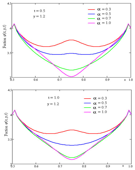
Figure 1. Profiles of function $\phi (x,1.2,t)$ for different values of the fractional parameter α, y = 1.2, t = 0.5 and t = 1.0.

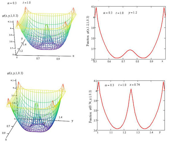
Figure 2. Profiles of surface $\phi (x,y,1)$ for $\alpha =0.3$ and their sections with the planes $y=1.2$ and $x=0.74$, respectively.

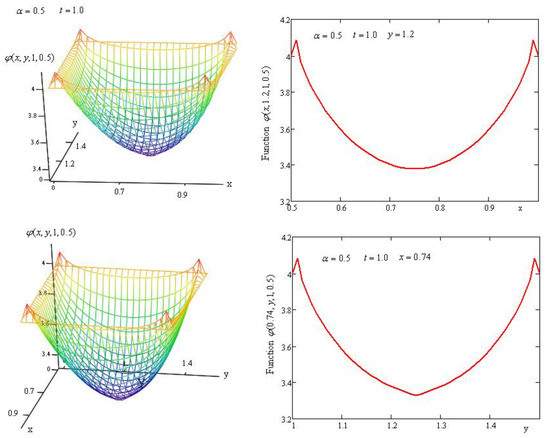
Figure 3. Profiles of surface $\phi (x,y,1)$ for $\alpha =0.5$ and their sections with the planes $y=1.2$ and $x=0.74$, respectively.

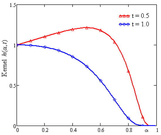
Figure 4. Profile of kernel $h(\alpha ,t)$ for two values of the time t.

To draw these graphs we have used the following values of the parameters: $a=0.5,b=1.0,c=1.0,d=1.5$, $p=0.25,{\gamma }_0=4,{\epsilon }_1={\epsilon }_2=0.2,k_1=0.25,k_2=0.5$.

In Figure 1, we show the plotted curves $\phi (x,1.2,0.5)$ and $\phi (x,1.2,1.0)$ for different values of the fractional parameter $\alpha \in \{0.3,0.5,0.7,1.0\}$. It is observed from Figure 1 that the values of concentration $\phi$ decrease with the fractional parameter and have a peak (maximum/minimum) in the central area of the geometrical domain $D=[a,b]\times [c,d]$.

In Figure 2 and Figure 3, we show the plotted surfaces $\phi (x,y,1)$ for the fractional parameters $\alpha =0.3$ and $\alpha =0.5$, respectively, along with the sections through planes $y=1.2,x=0.74$.

For small values of the fractional parameter, the concentration $\phi$ has maximum values in the central area of the rectangular $D=[a,b]\times [c,d]$. If the fractional parameter increases, the concentration has a minimum in the same area. This behavior is due to the kernel of the time-fractional Caputo–Fabrizio derivative (see Figure 4) which, for $t=0.5$, increases for $\alpha \le 0.55$ and decreases for $\alpha >0.55$. Therefore, at small values of the fractional parameter, the weight function in the fractional derivative has bigger values and the influence on the concentration is stronger.

5. Numerical Solution

In this section, based on the finite difference approximation of the derivatives, we develop a numerical scheme to the problem formulated in Section 2 of the paper.

We consider Equation (8) along with the initial and boundary conditions (10) and (11), with $(x,y,t)\in [a,b]\times [c,d]\times [0,T],T>0$. The discrete sets of nodes are defined as:

$$\begin{array}{l}{x}_i=a+i{h}_x,i=0,1,\dots ,N_1,h_x=(b-a)/N_1,\\ y_j=c+j{h}_y,j=0,1,\dots ,N_2,h_y=(d-c)/N_2,\\ t_n=n{h}_t,n=0,1,\dots ,N,h_t=T/N.\end{array}$$

(55)

The numerical estimation of the solution $\phi (x,y,t)$ of Equation (8) in the point $(x_i,y_j,t_n)$ is denoted by ${\phi }_{i,j}^n=\phi (x_i,y_j,t_n)$. The initial and boundary conditions (10) and (11) are written as:

$$\begin{array}{l}{\phi }_{i,j}^0=\phi (x_i,y_j,t_0)=0,i=0,1,\dots ,N_1,j=0,1,\dots ,N_2,\\ {\phi }_{0,j}^n=\phi (a,y_j,t_n)=F_1(a,y_j,t_n)+G_1(a,y_j)=P_{0,j}^n,j=0,1,\dots ,N_2,n=1,2,\dots ,N,\\ {\phi }_{N_1,j}^n=\phi (b,y_j,t_n)=F_1(b,y_j,t_n)+G_1(b,y_j)=Q_{N_1,j}^n,j=0,1,\dots ,N_2,n=1,2,\dots ,N,\\ {\phi }_{i,0}^n=\phi (x_i,c,t_n)=F_1(x_i,c,t_n)+G_1(x_i,c)=R_{i,0}^n,i=0,1,\dots ,N_1,n=1,2,\dots ,N,\\ {\phi }_{i,N_2}^n=\phi (x_i,d,t_n)=F_1(x_i,d,t_n)+G_1(x_i,d)=S_{i,N_2}^n,i=0,1,\dots ,N_1,n=1,2,\dots ,N,\end{array}$$

(56)

Using the following approximation for the first time-derivative:

$${\frac{\partial \phi (x_i,y_j,t)}{\partial t}|}_{t=t_k}=\frac{1}{h_t}\left[\phi (x_i,y_j,t_{k+1})-\phi (x_i,y_j,t_k)\right]=\frac{1}{h_t}\left({\phi }_{i,j}^{k+1}-{\phi }_{i,j}^k\right),k=0,1,\dots ,N-1,$$

(57)

the time-fractional Caputo–Fabrizio derivative, in the point $t=t_n$, can be approximated by:

$$\begin{array}{l}{{}^{CF}D_t^{\alpha }\phi \left(x,y,t\right)|}_{(x_i,y_j,t_n)}=\frac{1}{1-\alpha }{\displaystyle \underset{0}{\overset{t_n}{\int }}{\frac{\partial \phi (x_i,y_j,t)}{\partial t}|}_{t=\tau }}\exp \left(\frac{-\alpha (t_n-\tau )}{1-\alpha }\right)d\tau =\\ {\displaystyle \sum _{k=0}^{n-1}\frac{1}{1-\alpha }{\displaystyle \underset{t_k}{\overset{t_{k+1}}{\int }}{\frac{\partial \phi (x_i,y_j,t)}{\partial t}|}_{t=\tau }}\exp \left(\frac{-\alpha (t_n-\tau )}{1-\alpha }\right)d\tau }=\\ {\displaystyle \sum _{k=0}^{n-1}\frac{1}{(1-\alpha )h_t}\left({\phi }_{i,j}^{k+1}-{\phi }_{i,j}^k\right){\displaystyle \underset{t_k}{\overset{t_{k+1}}{\int }}\exp \left(\frac{-\alpha (t_n-\tau )}{1-\alpha }\right)d\tau }}={\displaystyle \sum _{k=0}^{n-1}{a}_{n,k}\left({\phi }_{i,j}^{k+1}-{\phi }_{i,j}^k\right)},n=1,2,\dots N,\end{array}$$

(58)

where

$$a_{n,k}=\frac{1}{\alpha h_t}\left[\exp \left(\frac{-\alpha (t_n-t_{k+1})}{1-\alpha }\right)-\exp \left(\frac{-\alpha (t_n-t_k)}{1-\alpha }\right)\right],\alpha \in (0,1),n=1,2,\dots ,N,k=0,1,\dots ,(n-1)$$

(59)

It is known [28,29] that Equation (58) approximates the time-fractional Caputo–Fabrizio derivative with an error of order $O(h_t^2)$.

The space derivatives of the second order are approximated by:

$$\begin{array}{l}{\frac{{\partial }^2\phi (x,y,t)}{\partial x^2}|}_{(x_i,y_j,t_n)}=\frac{1}{h_x^2}\left({\phi }_{i+1,j}^n-2{\phi }_{i,j}^n+{\phi }_{i-1,j}^n\right),i=1,2,\dots ,N_1-1,j=0,1,\dots ,N_2,n=1,2,\dots N,\\ {\frac{{\partial }^2\phi (x,y,t)}{\partial y^2}|}_{(x_i,y_j,t_n)}=\frac{1}{h_y^2}\left({\phi }_{i,j+1}^n-2{\phi }_{i,j}^n+{\phi }_{i,j-1}^n\right),i=0,1,\dots ,N_1,j=1,2,\dots ,N_2-1,n=1,2,\dots N.\end{array}$$

(60)

Using the approximation formulae (58) and (60), Equation (8) is written as:

$$\begin{array}{l}{\displaystyle \sum _{k=0}^{n-1}{a}_{n,k}\left({\phi }_{i,j}^{k+1}-{\phi }_{i,j}^k\right)+\beta {\phi }_{i,j}^n+{\beta }_1}\left({\phi }_{i+1,j}^n-2{\phi }_{i,j}^n+{\phi }_{i-1,j}^n\right)+\\ {\beta }_2\left({\phi }_{i,j+1}^n-2{\phi }_{i,j}^n+{\phi }_{i,j-1}^n\right)=H_{i,j}^n,i=1,2,\dots ,N_1-1,\cdots j=1,2,\dots ,N_2-1,n=1,2,\dots N,\end{array}$$

(61)

where

$${\beta }_1=\frac{-{\epsilon }_1}{h_x^2},{\beta }_2=\frac{-{\epsilon }_2}{h_y^2},H_{i,j}^n=F\left(x_i,y_j,t_n\right)+G\left(x_i,y_j\right)$$

(62)

For $n=1$, Equation (61) becomes:

$$d_{1,0}{\phi }_{i,j}^1+{\beta }_1\left({\phi }_{1+1,j}^1+{\phi }_{i-1,j}^1\right)+{\beta }_2\left({\phi }_{i,j+1}^1+{\phi }_{i,j-1}^1\right)=H_{i,j}^1,$$

(63)

where $d_{1,0}=a_{1,0}+\beta -2({\beta }_1+{\beta }_2)$.

Making $j=1$ and $i=1,2,\dots ,N_1-1$ into Equation (63), we obtain the following algebraic system:

$$\mathit{M}{\mathit{X}}_1+{\mathit{M}}_0{\mathit{X}}_2={\mathit{D}}_1^1,$$

(64)

where $\mathit{M}$ is a square matrix of order $(N_1-1)$ whose elements are given by:

$$\begin{array}{l}{M}_{0,k}=d_{1,0}{\delta }_{0,k}+{\beta }_1{\delta }_{1,k},k=0,1,\dots ,N_1-2,\\ M_{i,k}={\beta }_1{\delta }_{i,k+1}+d_{1,0}{\delta }_{i+1,k+1}+{\beta }_1{\delta }_{i+2,k+1},i=1,2,\dots ,N_1-2,k=k=0,1,\dots ,N_1-2,\end{array}$$

(65)

so,

$$\mathit{M}=\left(\begin{array}{ccccccccc}{d}_{1,0}& {\beta }_1& 0& 0& 0& \dots & 0& 0& 0\\ {\beta }_1& d_{1,0}& {\beta }_1& 0& 0& \dots & 0& 0& 0\\ 0& {\beta }_1& d_{1,0}& {\beta }_1& 0& \dots & 0& 0& 0\\ \dots & \dots & \dots & \dots & \dots & \dots & \dots & \dots & \dots \\ 0& 0& 0& 0& 0& \dots & {\beta }_1& d_{1,0}& {\beta }_1\\ 0& 0& 0& 0& 0& 0& \dots & {\beta }_1& d_{1,0}\end{array}\right)$$

(66)

the matrix ${\mathit{M}}_2$ is the diagonal square matrix of order $(N_1-1)$ with elements $M_{1i,j}={\beta }_2{\delta }_{i,j},i,j=0,1,\dots ,N_1-2,$ ${\delta }_{i,j}=\{\begin{array}{l}0,i\ne j,\\ 1,i=j,\end{array}$ is the Kronecker delta and ${\mathit{X}}_1,{\mathit{X}}_2{\mathit{D}}_1^1$ are the column-matrices.

$$\begin{array}{l}{\mathit{X}}_1=\left(\begin{array}{l}{\phi }_{1,1}^1\\ {\phi }_{2,1}^1\\ \dots \\ {\phi }_{N_1-1,1}^1\end{array}\right),{\mathit{X}}_2=\left(\begin{array}{l}{\phi }_{1,2}^1\\ {\phi }_{2,2}^1\\ \dots \\ {\phi }_{N_1-1,2}^1\end{array}\right),{\mathit{D}}_1^1=\left(\begin{array}{l}{D}_{11}^1\\ D_{12}^1\\ \dots \\ D_{1N_1-1}^1\end{array}\right),\begin{array}{c}{D}_{11}^1=H_{1,1}^1-{\beta }_1{P}_{0,1}^1-{\beta }_2{R}_{1,0}^1,\\ D_{1i}^1=H_{i,1}^1-{\beta }_2{R}_{i,0}^1,i=2,3,\dots ,N_1-2,\\ D_{1N_1-1}^1=H_{N_1-1,1}^1-{\beta }_1{Q}_{N_1,1}^1-{\beta }_2{R}_{N_1-1,0}^1.\end{array}\end{array}$$

(67)

The algebraic system (64) has $(N_1-1)$ equations with $2(N_1-1)$ unknown functions.

Making $j=2,3,\dots ,N_2-2$ and $i=1,2,\dots ,N_1-1$ into Equation (63), we obtain the algebraic system:

$${\mathit{M}}_0{\mathit{X}}_{j-1}+\mathit{M}{\mathit{X}}_j+{\mathit{M}}_0{\mathit{X}}_{j+1}={\mathit{D}}_j^1,$$

(68)

where

$$\begin{array}{l}{D}_{j1}^1=H_{1,j}^1-{\beta }_1{P}_{0,j}^1,\\ D_{ji}^1=H_{i,j}^1,i=2,3,\dots ,N_1-2,\\ D_{j{N}_1-1}^1=H_{N_1-1.j}^1-{\beta }_1{Q}_{N_1,j}^1.\end{array}$$

(69)

Making $j=N_2-1$ and $i=1,2,\dots ,N_1-1$ into Equation (63), we obtain the algebraic system:

$${\mathit{M}}_0{\mathit{X}}_{N_2-2}+\mathit{M}{\mathit{X}}_{N_2-1}={\mathit{D}}_{N_2-1}^1,$$

(70)

where

$$\begin{array}{l}{D}_{N_2-11}^1=H_{1,N_2-1}^1-{\beta }_1{P}_{0,N_2-1}^1-{\beta }_2{S}_{1,N_2}^1,\\ D_{N_2-1i}^1=H_{i,N_2-1}^1-{\beta }_2{S}_{i,N_2}^1,i=2,3,\dots ,N_1-2,\\ D_{N_2-1N_1-1}^1=H_{N_1-1.N_2-1}^1-{\beta }_1{Q}_{N_1,N_2-1}^1-{\beta }_2{S}_{N_1-1,N_2}^1.\end{array}$$

(71)

The algebraic systems (64), (68) and (70) can be written as a unique algebraic system of $(N_1-1)(N_2-1)$ equations with $(N_1-1)(N_2-1)$ unknown functions ${\phi }_{i,j}^1,i=1,2,\dots ,N_1-1,j=1,2,\dots ,N_2-1$, namely

$$\left(\begin{array}{ccccccccc}\mathit{M}& {\mathit{M}}_0& 0& 0& 0& \dots & 0& 0& 0\\ {\mathit{M}}_0& \mathit{M}& {\mathit{M}}_0& 0& 0& \dots & 0& 0& 0\\ 0& {\mathit{M}}_0& \mathit{M}& {\mathit{M}}_0& 0& \dots & 0& 0& 0\\ \dots & \dots & \dots & \dots & \dots & \dots & \dots & \dots & \dots \\ 0& 0& 0& 0& 0& \dots & {\mathit{M}}_0& \mathit{M}& {\mathit{M}}_0\\ 0& 0& 0& 0& 0& 0& \dots & {\mathit{M}}_0& \mathit{M}\end{array}\right)\left(\begin{array}{l}{X}_1\\ X_2\\ X_3\\ \dots \\ X_{N_2-2}\\ X_{N_2-1}\end{array}\right)=\left(\begin{array}{l}{D}_1^1\\ D_2^1\\ D_3^1\\ \dots \\ D_{N_2-2}^1\\ D_{N_2-1}^1\end{array}\right)$$

(72)

The solution of system (72) gives the values of function $\phi (x,y,t)$ in points $(x_i,y_j,t_1)$ for $i=1,2,\dots ,N_1-1,j=1,2,\dots ,N_2-1$.

The numerical procedure is continued in a similar way for $n=2,3,\dots ,N$ when Equation (61) is written in the equivalent form:

$$d_{n,n-1}{\phi }_{i,j}^n+{\beta }_1\left({\phi }_{i+1,j}^n+{\phi }_{i-1,j}^n\right)+{\beta }_2\left({\phi }_{i,j+1}^n+{\phi }_{i,j-1}^n\right)=G_{i,j}^n,i=1,2,\dots ,N_1-1,j=1,2,\dots ,N_2-1,$$

(73)

where

$$\begin{array}{l}{d}_{n,n-1}=a_{n,n-1}+\beta -2({\beta }_1+{\beta }_2),n=2,3,\dots ,N,\\ G_{i,j}^n=H_{i,j}^n+a_{n,n-1}{\phi }_{i,j}^{n-1}-{\displaystyle \sum _{k=0}^{n-2}{a}_{n,k}\left({\phi }_{i,j}^{k+1}-{\phi }_{i,j}^k\right)},i=1,2,\dots ,N_1-1,j=1,2,\dots ,N_2-1.\end{array}$$

(74)

Finally, the proposed numerical procedure gives the values of the solution $\phi (x,y,t)$ in grid points $(x_i,y_j,t_n),i=1,2,\dots ,N_1-1,j=1,2,\dots ,N_2-1,n=1,2,\dots ,N$.

To compare the numerical values obtained with the analytical solution, respectively, by the numerical method, we have considered the following particular problem:

$$\begin{array}{l}F(x,y,t)=5000\exp \left(-\frac{k_{1}x}{2{\epsilon }_1}-\frac{k_{2}y}{2{\epsilon }_2}\right),G(x,y)=0,(x,y,t)\in [0,0.05]\times [0,0.05]\times [0,0.1],\\ F_1(x,y,t)=0,G_1(x,y)=0,\phi (x,y,0)=0,\\ k_1=k_2=0.5,{\epsilon }_1={\epsilon }_2=2,\end{array}$$

(75)

In this case, the double Fourier transform of the function $F(x,y,t)$ is:

$$\begin{array}{cc}\hfill \tilde{F}(n,k)=& \frac{n\pi (b-a)\left[\exp \left(\frac{-a{k}_1}{2{\epsilon }_1}\right)-{(-1)}^n\exp \left(\frac{-b{k}_1}{2{\epsilon }_1}\right)\right]}{{\left(\frac{k_1}{2{\epsilon }_1}\right)}^2{(b-a)}^2+{(n\pi )}^2}\times \hfill \\ & \frac{k\pi (b-a)\left[\exp \left(\frac{-c{k}_2}{2{\epsilon }_2}\right)-{(-1)}^k\exp \left(\frac{-d{k}_2}{2{\epsilon }_2}\right)\right]}{{\left(\frac{k_2}{2{\epsilon }_2}\right)}^2{(d-c)}^2+{(k\pi )}^2},\hfill \end{array}$$

(76)

and the analytical solution is given by:

$$\begin{array}{l}\phi (x,y,t)=\frac{4\alpha }{\left(b-a\right)\left(d-c\right)}{\displaystyle \sum _{n=1}^{\infty }{\displaystyle \sum _{k=1}^{\infty }\frac{\tilde{F}(n,k)}{b_{nk}}\sin \left[\frac{n(x-a)\pi }{b-a}\right]}}\sin \left[\frac{k(y-c)\pi }{d-c}\right]+\\ \frac{4}{\left(b-a\right)\left(d-c\right)}{\displaystyle \sum _{n=1}^{\infty }{\displaystyle \sum _{k=1}^{\infty }\frac{\tilde{F}(n,k)\left[(1-\alpha )b_{nk}-\alpha a_{nk}\right]}{a_{nk}{b}_{nk}}\sin \left[\frac{n(x-a)\pi }{b-a}\right]}}\sin \left[\frac{k(y-c)\pi }{d-c}\right]{\mathrm{e}}^{-\frac{b_{nk}t}{a_{nk}}}.\end{array}$$

(77)

The values of function $\phi (x,y,t)$ at the instant $t=0.01$, obtained with the numerical method and with expression (77) given in the Table 1, are in good agreement.

Table 1. Values of function $\phi (x,y,0.01)$.

x	$y_1=0.005$		$y_2=0.010$		$y_3=0.015$
	Numerical Solution	Equation (77)	Numerical Solution	Equation (77)	Numerical Solution	Equation (77)
0.005	0.080	0.081	0.129	0.130	0.158	0.159
0.010	0.129	0.130	0.214	0.216	0.267	0.270
0.015	0.158	0.159	0.267	0.270	0.338	0.340
0.020	0.174	0.175	0.297	0.299	0.379	0.381
0.025	0.179	0.181	0.307	0.309	0.391	0.394
0.030	0.174	0.175	0.297	0.299	0.378	0.381
0.035	0.158	0.159	0.268	0.269	0.338	0.340
0.040	0.125	0.120	0.213	0.215	0.267	0.270
0.045	0.080	0.081	0.129	0.130	0.158	0.159
x	$y_4=0.020$		$y_5=0.025$		$y_6=0.030$
	Numerical Solution	Equation (77)	Numerical Solution	Equation (77)	Numerical Solution	Equation (77)
0.005	0.174	0.175	0.179	0.181	0.174	0.175
0.010	0.297	0.299	0.306	0.309	0.297	0.299
0.015	0.378	0.380	0.391	0.394	0.379	0.381
0.020	0.424	0.427	0.439	0.441	0.424	0.427
0.025	0.439	0.441	0.455	0.457	0.438	0.442
0.030	0.423	0.426	0.438	0.441	0.423	0.426
0.035	0.377	0.380	0.391	0.393	0.377	0.380
0.040	0.296	0.298	0.306	0.308	0.296	0.299
0.045	0.174	0.175	0.179	0.181	0.174	0.175
x	$y_7=0.035$		$y_8=0.040$		$y_9=0.045$
	Numerical Solution	Equation (77)	Numerical Solution	Equation (77)	Numerical Solution	Equation (77)
0.005	0.158	0.159	0.128	0.130	0.080	0.081
0.010	0.267	0.269	0.213	0.215	0.128	0.130
0.015	0.338	0.340	0.267	0.269	0.158	0.159
0.020	0.377	0.380	0.296	0.298	0.174	0.175
0.025	0.390	0.393	0.306	0.308	0.179	0.180
0.030	0.377	0.380	0.296	0.299	0.174	0.175
0.035	0.337	0.340	0.266	0.269	0.157	0.159
0.040	0.266	0.269	0.212	0.214	0.128	0.129
0.045	0.157	0.159	0.128	0.129	0.079	0.081

6. Discussion and Conclusions

A two-dimensional advection–diffusion process with short-tail memory and concentrated source situated in the symmetry center of the geometrical domain has been investigated.

The studied mathematical model is described by a fractional differential equation with a time-fractional Caputo–Fabrizio derivative with exponential kernel.

Analytical solutions of the proposed initial-boundary value problem were obtained using the integral transform method (Laplace and finite Fourier transforms are employed).

Numerical solutions of the studied problem have been determined using finite difference approximations.

Numerical simulations for both analytical and numerical solutions have been carried out using the software Mathcad.

The fractional order of the Caputo–Fabrizio derivative has a significant influence on the pollutant concentration. For small values of the fractional parameter, the concentration has maximum values in the central area of the geometrical domain. If the fractional parameter increases, the concentration has a minimum in the same area. This behavior is due to the memory kernel of the time-fractional Caputo–Fabrizio derivative.

References

- Mainardi, F. Fractals and Fractional Calculus in Continuum Mechanics; Springer: Wien, Austria, 1997. [Google Scholar]
- Laskin, N. Fractional Quantum Mechanics; World Scientific: Hackensack, NJ, USA, 2018. [Google Scholar]
- Laskin, N. Generalized classical mechanics. Eur. Phys. J. Spec. Top. 2013, 222, 1929–1938. [Google Scholar] [CrossRef]
- Hristov, J. Fractional derivative with non-singular kernels: From the Caputo-Fabrizio definition and beyond: Appraising analysis with emphasis on diffusion models. In Frontiers in Fractional Calculus; Bhalekar, S., Ed.; Bentham Publication: Kolhapur, India, 2017; Chapter 10; pp. 243–269. [Google Scholar]
- Baleanu, D.; Golmankhaneh, A.K.; Nigmatullin, R.; Golmankhaneh, A.K. Fractional Newtonian mechanics. Cent. Eur. J. Phys. 2010, 8, 120–125. [Google Scholar] [CrossRef]
- Povstenko, Y. Fractional Thermoelasticity, Solid Mechanics and Its Applications; Springer International Publishing: Cham, Switzerland, 2015; p. 219. [Google Scholar]
- Bhrawy, A.H.; Baleanu, D. A spectral Legendre-Gauss-Lobatto collocation method for a space-fractional advection diffusion equation with variable coefficients. Rep. Math. Phys. 2013, 72, 219–233. [Google Scholar] [CrossRef]
- Abdelkawy, M.A.; Zaky, M.A.; Bhrawy, A.H.; Baleanu, D. Numerical simulation of time variable fractional order mobile-immobile advection-dispersion model. Rom. Rep. Phys. 2015, 67, 773–791. [Google Scholar]
- Zhuang, P.; Liu, F.; Anh, V.; Turner, I. Numerical methods for the variable-order fractional advection-diffusion equation with a nonlinear source term. SIAM J. Num. Anal. 2009, 47, 1760–1781. [Google Scholar] [CrossRef]
- Fazio, R.; Jannelli, A.; Agreste, S. A finit difference method on non-uniform meshes for time-fractional advection-diffusion equations with a source term. Appl. Sci. 2018, 8, 960. [Google Scholar] [CrossRef]
- Arshad, S.; Baleanu, D.; Huang, J.; Al Qurashi, M.M.; Tang, Y.; Zhao, Y. Finite difference method for time-space fractional advection-diffusion equations with Riesz derivative. Entropy 2018, 20, 321. [Google Scholar] [CrossRef]
- Jannelli, A.; Ruggieri, M.; Speciale, M.P. Exact and numerical solutions of time-fractional advection-diffusion equation with a nonlinear source term by means of the Lie symmetries. Nonlinear Dyn. 2018, 92, 543–555. [Google Scholar] [CrossRef]
- Badr, M.; Yazdani, A.; Jafari, H. Stability of a finite volume element method for the time-fractional advection-diffusion equation. Numer. Methods Partial Differ. Eqs. 2018, 34, 1459–1471. [Google Scholar] [CrossRef]
- Pimenov, V.G. Numerical method for advection-diffusion equation with heredity. Itogi Naukii Tekniki Ser. Sovrem. Mat. Pril. Temat. Obz. 2017, 132, 86–90. [Google Scholar] [CrossRef]
- Singh, J.; Secer, A.; Swroop, R.; Kumar, D. A reliable analytical approach for a fractional model of advection-dispersion equation. Nonlinear Eng. 2018, in press. [Google Scholar] [CrossRef]
- Avci, D.; Yetim, A. Analytical solution to the advection-diffusion equation with the Atangana-Baleanu derivative over a finite domain. J. BAUN Inst. Sci. Technol. 2018, 20, 382–395. [Google Scholar] [CrossRef]
- Mirza, I.A.; Vieru, D. Fundamental solutions to advection-diffusion equation with time-fractional Caputo-Fabrizio derivative. Comput. Math. Appl. 2017, 73, 1–10. [Google Scholar] [CrossRef]
- Mirza, I.A.; Vieru, D.; Ahmed, N. Fractional advection-diffusion equation with memory and Robin-type boundary condition. Math. Model. Nat. Phenom. 2019, 14, 306. [Google Scholar] [CrossRef]
- Hristov, J. Integral balance approach to 1-D space-fractional diffusion models. In Mathematical Methods in Engineering Applications in Dynamics of Complex Systems; Tas, K., Baleanu, D., Machado, J.A.T., Eds.; Springer: Cham, Switzerland, 2019; pp. 1–21. [Google Scholar]
- Hristov, J. The heat radiation diffusion equation with memory: Constitutive approach and approximate integral-balance solutions. In Heat Conduction, Methods, Applications and Research; Hristov, J., Bennacer, R., Eds.; NOVA Science Publishers: New York, NY, USA, 2019. [Google Scholar]
- Hristov, J. Response functions in linear viscoelastic constitutive equations and related fractional operators. Math. Model. Nat. Phenom. 2018, 14, 305. [Google Scholar] [CrossRef]
- Povstenko, Y.; Klekot, J. The Dirichlet problem for the time-fractional advection-diffusion equation in a line segment. Bound. Value Probl. 2016, 2016, 89. [Google Scholar] [CrossRef]
- Povstenko, Y.; Kyrylych, T. Time-fractional diffusion with mass absorption in a half-space line domain due to boundary value of concentration varying harmonically in time. Entropy 2018, 19, 346. [Google Scholar] [CrossRef]
- Fulger, D.; Scalas, E.; Germano, G. Monte Carlo simulation of uncoupled continuous-time random walks yielding a stochastic solution of the space-time fractional diffusion equation. Phys. Rev. E 2008, 77, 021122. [Google Scholar] [CrossRef]
- Caputo, M.; Fabrizio, M. A new definition of fractional derivative without singular kernel. Progr. Fract. Differ. Appl. 2015, 1, 73–85. [Google Scholar]
- Andrews, L.C.; Shivamoggi, B.K. Integral Transforms for Engineers; SPIE Press: Washington, DC, USA, 1999. [Google Scholar]
- Bracewell, R. The Shifting Property. In The Fourier Transform and Its Applications, 3rd ed.; McGraw-Hill Science/Engineering/Math.: New York, NY, USA, 1999; pp. 74–77. [Google Scholar]
- Atangana, A.; Alqahtani, R.T. Numerical approximation of the space-time Caputo-Fabrizio fractional derivative and application to groundwater pollution equation. Adv. Diff. Eqs. 2016, 2016, 156. [Google Scholar] [CrossRef]
- Rangaig, N.A. Finite difference approximation for Caputo-Fabrizio time fractional derivative on non-uniform mesh and some applications. Phys. J. 2018, 3, 255–263. [Google Scholar]
© 2019 by the authors. Licensee MDPI, Basel, Switzerland. This article is an open access article distributed under the terms and conditions of the Creative Commons Attribution (CC BY) license (http://creativecommons.org/licenses/by/4.0/).