Robust Nonparametric Methods of Statistical Analysis of Wind Velocity Components in Acoustic Sounding of the Lower Layer of the Atmosphere


Abstract
:1. Introduction
2. Procedure of Outlier Detection and Selection
2.1. Adaptive Pendular Truncation Algorithm
2.2. Adaptive Pendular Truncation Algorithm
- Calculate ,
- Calculate ,
- Sort the variables , ,
- Calculate ,
- Calculate ,
- Find the first-order differences ,
- Find the second-order differences ,
- Remove the observation corresponding to from the sample,
- Execute the above cycle from item 1 to item 9 for .
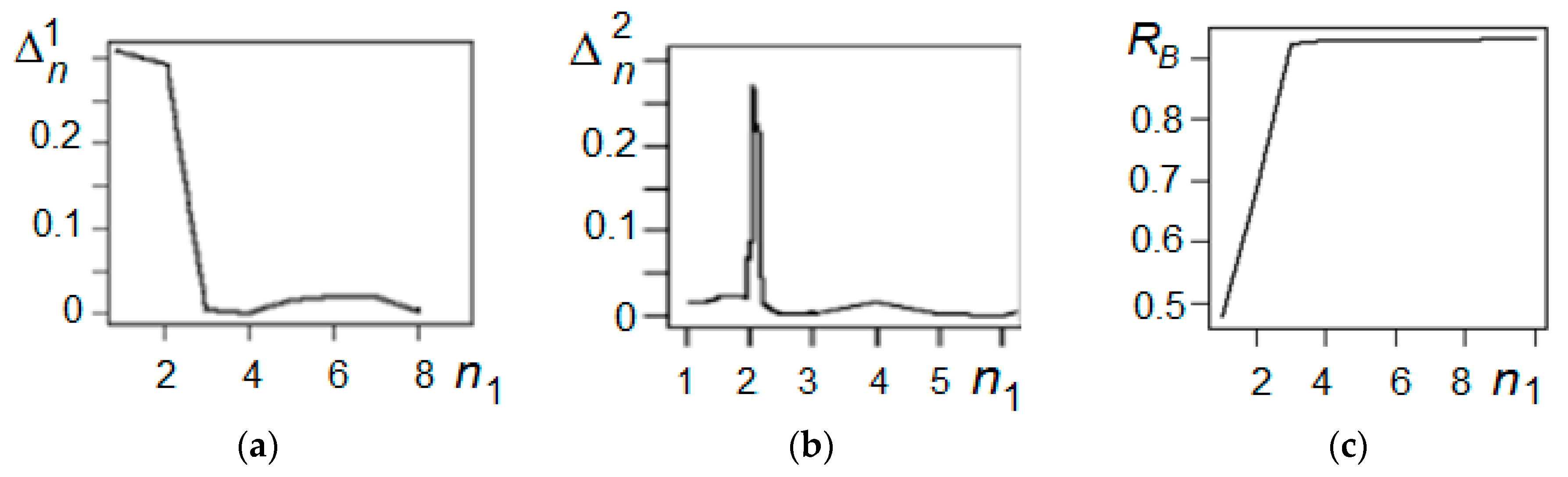
Generalization of the Algorithm
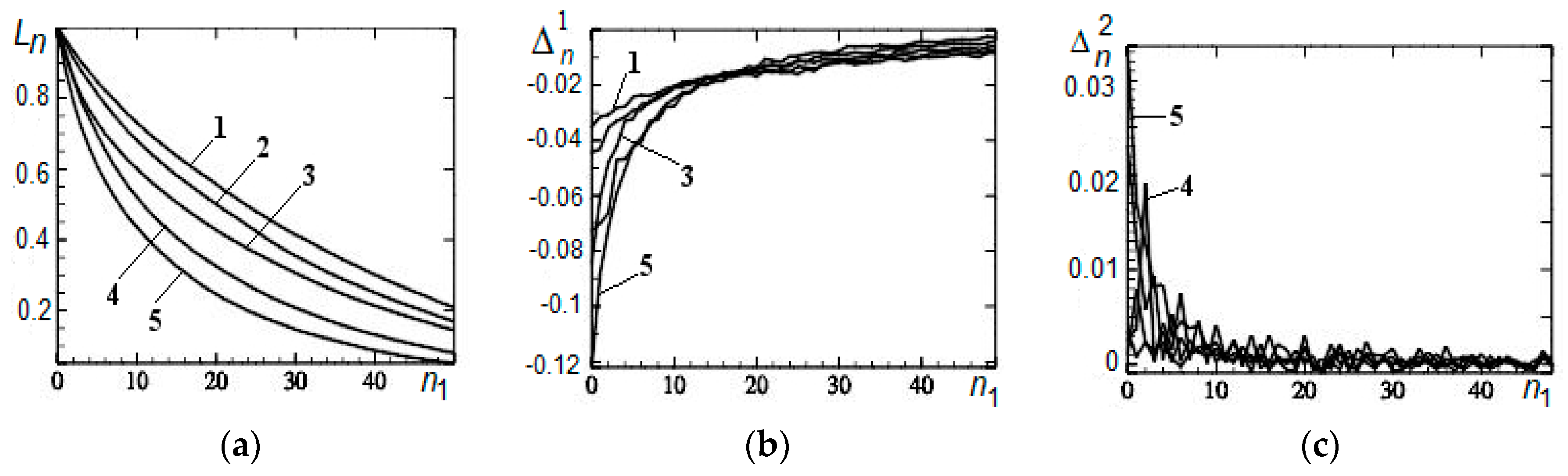
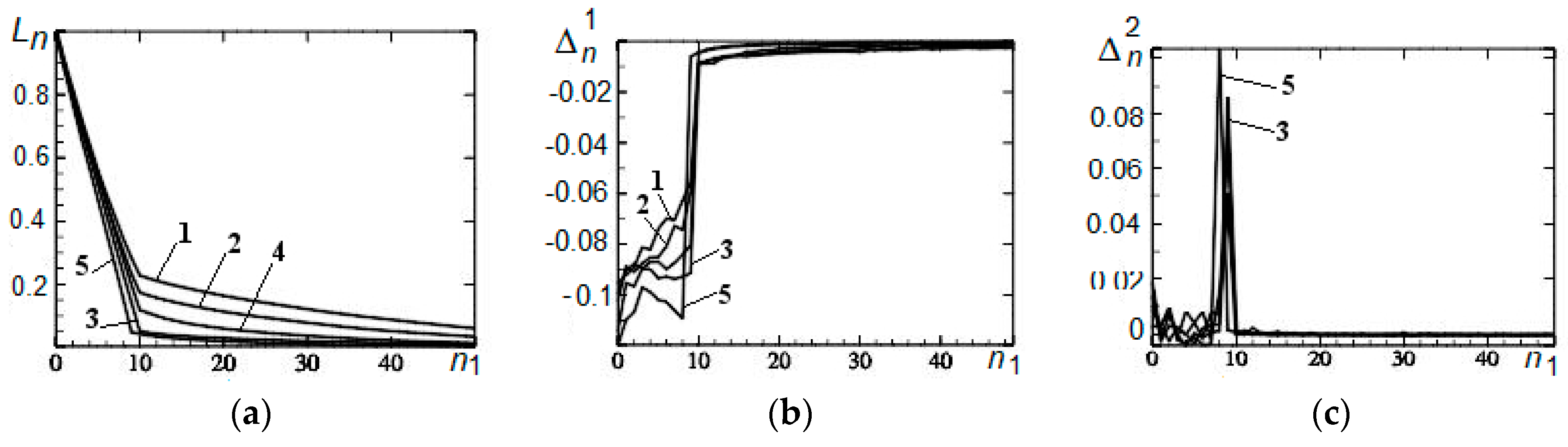
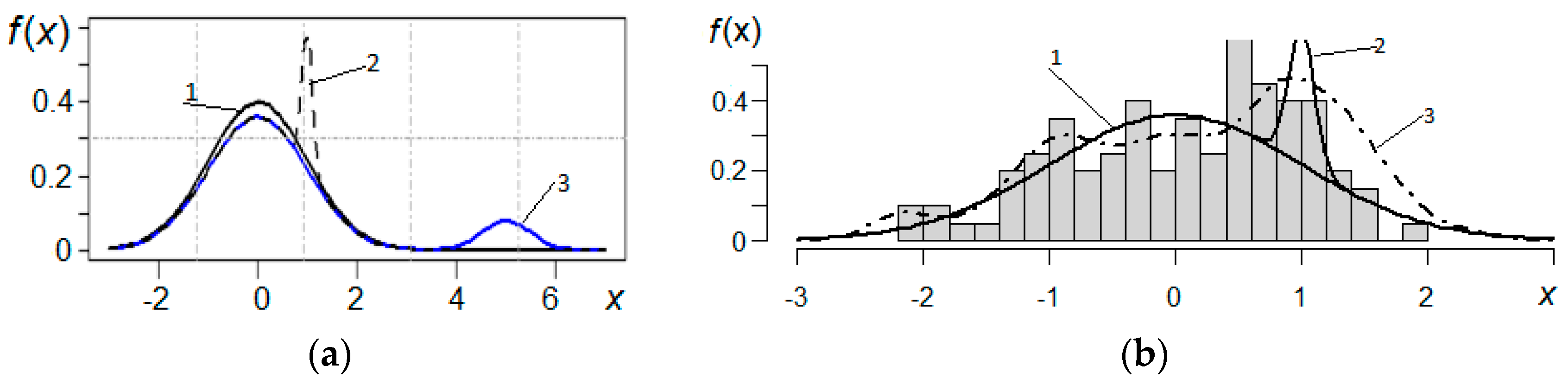
3. Simulation
3.1. Remote Outliers
3.2. Asymmetry
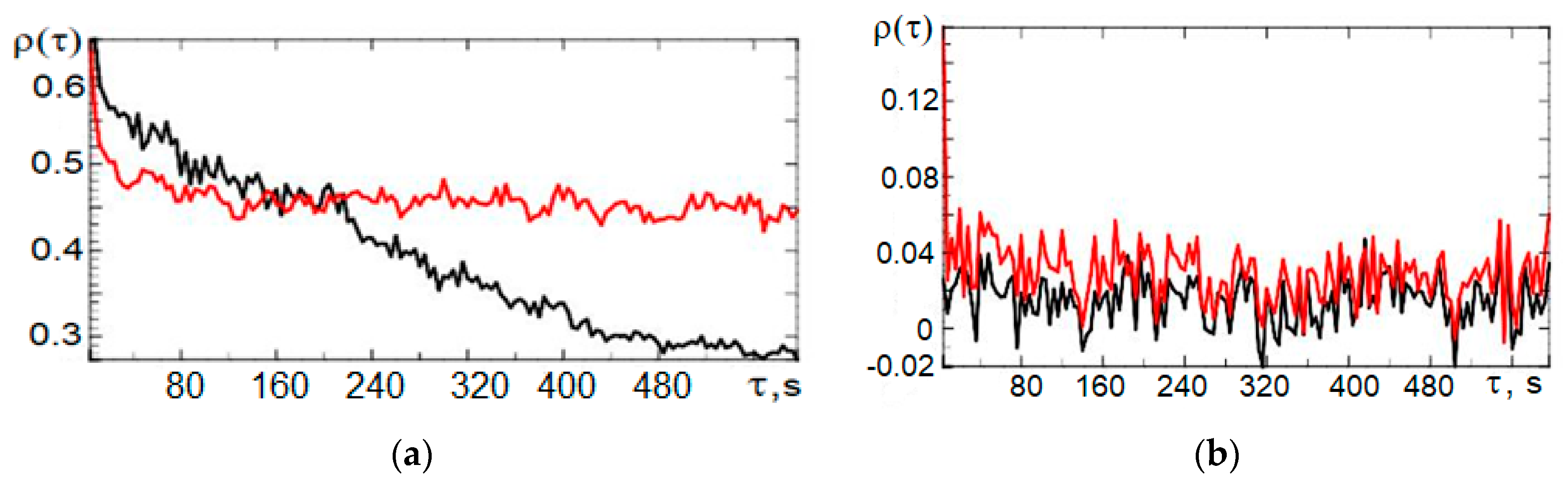
3.3. Correlation
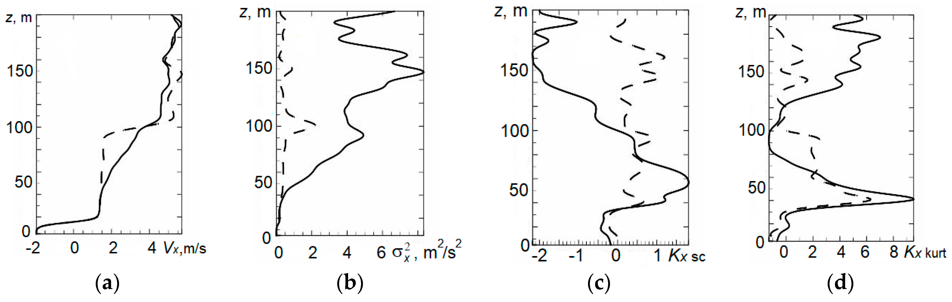
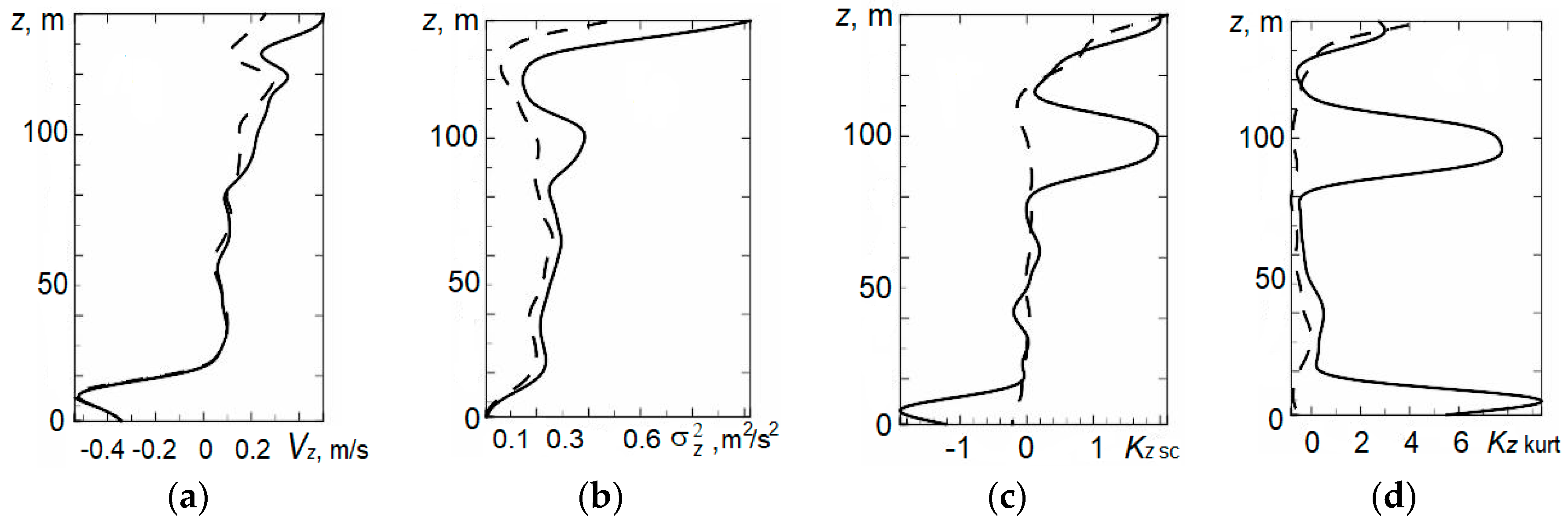
4. Statistical Analysis of Vertical Profiles of Wind Velocity Components from Results of Minisodar Measurements using the Pendular Truncation Algorithm
5. Conclusions
Author Contributions
Funding
Conflicts of Interest
References
- Singal, S.P. Acoustic Remote-Sensing Applications; Springer-Verlag: Berlin, Germany, 1997; p. 585. [Google Scholar]
- Kallistratova, M.A.; Kon, A.I. Radioacoustic Sounding of the Atmosphere; Nauka: Moscow, Russia, 1985; p. 197. (In Russian) [Google Scholar]
- Krasnenko, N.P. Acoustic Sounding of the Atmosphere; Nauka: Novosibirsk, Russia, 1986; p. 168. (In Russian) [Google Scholar]
- Krasnenko, N.P. Acoustic Sounding of the Atmospheric Boundary Layer; Vodolei: Tomsk, Russia, 2001; p. 279. (In Russian) [Google Scholar]
- Bradley, S. Atmospheric Acoustic Remote Sensing: Principles and Applications; CRC Press Taylor & Francis Group: Boca Raton, FL, USA, 2007; p. 296. [Google Scholar]
- Simakhin, V.A.; Cherepanov, O.S.; Shamanaeva, L.G. Spatiotemporal dynamics of the wind velocity from minisodar measurement data. Russ. Phys. J. 2015, 58, 176–181. [Google Scholar] [CrossRef]
- Hampel, F.; Ronchetti, E.; Rausseu, P.; Shtael, V. Robustness in Statistics. Approach Based on Influence Functions; MIR: Moscow, Russia, 1989; p. 512, (Russian translation). [Google Scholar]
- Shulenin, V.P. Methods of Mathematical Statistics; Publishing House of Scientific and Technology Literature: Tomsk, Russia, 2016; p. 260. (In Russian) [Google Scholar]
- Muthukrishnan, R.; Poonkuzhali, G. A comprehensive survey on outlier detection methods. Am. -Eurasian J. Sci. Res. 2017, 12, 161–171. [Google Scholar]
- Chandola, V.; Banerjee, A.; Kumar, V. Anomaly detection: A survey. ACM Comput. Surv. 2009, 41, 1–83. [Google Scholar] [CrossRef]
- Hodge, V.; Austin, J. A survey of outlier detection methodologies. Artif. Intell. Rev. 2004, 22, 85–126. [Google Scholar] [CrossRef]
- Grubbs, F.E. Sample criteria for testing outlying observations. Ann. Math. Stat. 1950, 21, 27–58. [Google Scholar] [CrossRef]
- Tietjen, G.L.; Moore, R.H. Some Grubbs-type statistics for the detection of several outliers. Technometrics 1972, 14, 583–597. [Google Scholar] [CrossRef]
- Rosner, B. On the detection of many outliers. Technometrics 1975, 17, 221–227. [Google Scholar] [CrossRef]
- Ferguson, T.S. On the rejection of outliers. In Proceedings of the Fourth Berkeley Symposium on Mathematical Statistics and Probability, Berkeley, CA, USA, 20–30 July 1961; Volume 1, pp. 253–287. [Google Scholar]
- Orlov, A.I. Instability of parametric methods of rejection of sharply allocated observations. Zavod. Lab. 1992, 7, 40–42. (In Russian) [Google Scholar]
- Rocke, D.M.; Woodruff, D.L. Identification of outliers in multivariate data. J. Am. Stat. Assoc. 2012, 91, 1047–1061. [Google Scholar] [CrossRef]
- Shevlyakov, G.L.; Vilchevski, N.O. Robustness in Data Analysis: Criteria and Methods; VSP: Utrecht, The Netherlands, 2002; p. 315. [Google Scholar]
- Fedorov, V.A. Measurements with the “Volna-3” sodar of the parameters of radial components of wind velocity vector. Atmos. Ocean. Opt. 2003, 16, 151–155. [Google Scholar]
- Simakhin, V.A.; Cherepanov, O.S. Detection and selection of signal outliers. In Proceedings of the XIX International Symposium “Atmospheric and Oceanic Optics. Atmospheric Physics”, Barnaul, Russia, 1–3 July 2013; pp. С221–С224. (In Russian). [Google Scholar]
- Huber, P.J. Robust Statistics; Willey: New York, NY, USA, 1981; p. 308. [Google Scholar]
- Simakhin, V.A. Robust Nonparametric Estimates; Lambert Academic Publishing: Saarbrücken, Germany, 2011; p. 292. [Google Scholar]
- Krasnenko, N.P.; Tarasenkov, M.V.; Shamanaeva, L.G. Spatiotemporal dynamics of the wind velocity from data of sodar measurements. Russ. Phys. J. 2014, 57, 1539–1546. [Google Scholar] [CrossRef]


© 2019 by the authors. Licensee MDPI, Basel, Switzerland. This article is an open access article distributed under the terms and conditions of the Creative Commons Attribution (CC BY) license (http://creativecommons.org/licenses/by/4.0/).
Share and Cite
Krasnenko, N.; Simakhin, V.; Shamanaeva, L.; Cherepanov, O. Robust Nonparametric Methods of Statistical Analysis of Wind Velocity Components in Acoustic Sounding of the Lower Layer of the Atmosphere. Symmetry 2019, 11, 961. https://doi.org/10.3390/sym11080961
Krasnenko N, Simakhin V, Shamanaeva L, Cherepanov O. Robust Nonparametric Methods of Statistical Analysis of Wind Velocity Components in Acoustic Sounding of the Lower Layer of the Atmosphere. Symmetry. 2019; 11(8):961. https://doi.org/10.3390/sym11080961
Chicago/Turabian StyleKrasnenko, Nikolay, Valerii Simakhin, Liudmila Shamanaeva, and Oleg Cherepanov. 2019. "Robust Nonparametric Methods of Statistical Analysis of Wind Velocity Components in Acoustic Sounding of the Lower Layer of the Atmosphere" Symmetry 11, no. 8: 961. https://doi.org/10.3390/sym11080961
APA StyleKrasnenko, N., Simakhin, V., Shamanaeva, L., & Cherepanov, O. (2019). Robust Nonparametric Methods of Statistical Analysis of Wind Velocity Components in Acoustic Sounding of the Lower Layer of the Atmosphere. Symmetry, 11(8), 961. https://doi.org/10.3390/sym11080961