1. Introduction
Finding numerically a root of an equation is an interesting and challenging problem. It is also very important in many diverse areas such as Mathematical Biology, Physics, Chemistry, Economics and Engineering, to name a few [
1,
2,
3,
4]. This is due to the fact that many problems from these disciplines are ultimately reduced to finding the root of an equation. Researchers are using iterative methods for approximating root since closed form solutions cannot be obtained in general. In particular, here we consider the problem of computing multiple roots of equation
by iterative methods. A root (say,
) of
is called multiple root with multiplicity
m, if
and
.
A basic and widely used iterative method is the well-known modified Newton’s method
This method efficiently locates the required multiple root with quadratic order of convergence provided that the initial value
is sufficiently close to root [
5]. In terms of Traub’s classification (see [
1]), Newton’s method (
1) is called one-point method. Some other important methods that belong to this class have been developed in [
6,
7,
8,
9].
Recently, numerous higher order methods, either independent or based on the modified Newton’s method (
1), have been proposed and analyzed in the literature, see e.g., [
10,
11,
12,
13,
14,
15,
16,
17,
18,
19,
20,
21,
22,
23] and references cited therein. Such methods belong to the category of multipoint methods [
1]. Multipoint iterative methods compute new approximations to root
by sampling the function
, and its derivatives at several points of the independent variable, per each step. These methods have the strategy similar to Runge–Kutta methods for solving differential equations and Gaussian quadrature integration rules in the sense that they possess free parameters which can be used to ensure that the convergence speed is of a certain order, and that the sampling is done at some suitable points.
In particular, Geum et al. in [
22,
23] have proposed two- and three-point Newton-like methods with convergence order six for finding multiple roots. The two-point method [
22], applicable for
, is given as
where
and
and
is a holomorphic function in some neighborhood of origin
. The three-point method [
23] for
is given as
wherein
and
. The function
is analytic in a neighborhood of 0 and
is holomorphic in a neighborhood of
. Both schemes (
2) and (
3) require four function evaluations to obtain sixth order convergence with the efficiency index (see [
24]),
.
The goal and motivation in constructing iterative methods is to attain convergence of order as high as possible by using function evaluations as small as possible. With these considerations, here we propose a family of three-point methods that attain seventh order of convergence for locating multiple roots. The methodology is based on Newton’s and weighted-Newton iterations. The algorithm requires four evaluations of function per iteration and, therefore, possesses the efficiency index
. This shows that the proposed methods have better efficiency
than the efficiency
of existing methods (
2) and (
3). Theoretical results concerning convergence order and computational efficiency are verified by performing numerical tests. In the comparison of numerical results with existing techniques, the proposed methods are observed computationally more efficient since they require less computing time (CPU-time) to achieve the solution of required accuracy.
Contents of the article are summarized as follows. In
Section 2, we describe the approach to develop new methods and prove their seventh order convergence. In
Section 3, stability of the methods is checked by means of using a graphical technique called basins of attraction. In
Section 4, some numerical tests are performed to verify the theoretical results by implementing the methods on some examples. Concluding remarks are reported in
Section 5.
2. Formulation of Method
Let
be the multiplicity of a root of the equation
. To compute the root let us consider the following three-step iterative scheme:
where
,
,
, and the function
is analytic in some neighborhood of 0 and
is holomorphic in a neighborhood of
. Notice that the first step is Newton iteration (
1) whereas second and third steps are weighted by employing the factors
and
, and so we call the algorithm (
4) by the name weighted-Newton method. Factors
H and
G are called weight factors or more appropriately weight functions.
In the sequel we shall find conditions under which the algorithm (
4) achieves high convergence order. Thus, the following theorem is stated and proved:
Theorem 1. Assume that is an analytic function in a domain enclosing a root α with multiplicity m. Suppose that initial point is closer enough to the root α, then the iterative formula defined by (4) has seventh order of convergence, if the functions and verify the conditions: , , , , where . Proof. Let
be the error at
n-th iteration. Taking into account that
,
, we have by the Taylor’s expansion of
about
or:
where
for
.
also
where
for
.
Using (
5) and (
6) in first step of (
4), it follows that
where
are given in terms of
with explicitly written two coefficients
,
. Here, rest of the expressions of
are not being produced explicitly since they are very lengthy.
Expansion of
about
yields
where
Using (
5) and (
8) in the expression of
u, it follows that
where
with explicitly written one coefficient
.
Developing weight function
in neighborhood 0,
Inserting Equations (
5), (
8) and (
10) in the second step of (
4), after some simplifications we have that
where
and
.
In order to accelerate convergence, the coefficients of
and
should be equal to zero. That is possible only if we have
By using the above values in (
11), we obtain that
Expansion of
about
yields
From (
5), (
8) and (
14), we obtain forms of
v and
w as
where
and
where
.
Expanding
in neighborhood of origin
by Taylor series, it follows that
where
.
Then by substituting (
5), (
6), (
15)–(
17) into the last step of scheme (
4), we obtain that
where
.
From Equation (
18) it is clear that we can obtain at least fifth order convergence when
. In addition, using this value in
, we will obtain that
By using
and (
19) in
, the following equation is obtained
which further yields
Using the above values in (
18), we obtain the error equation
Thus, the seventh order convergence is established. □
Based on the conditions on
and
as shown in Theorem 1, we can generate numerous methods of the family (
4). However, we restrict to the following simple forms:
2.1. Some Concrete Forms of
Case 1.Considering a polynomial function, i.e., Using the conditions of Theorem 1, we get , and . Then Case 2.When is a rational function, i.e., Using the conditions of Theorem 1, we get that , and . So Case 3.Consider as another rational weight function, e.g., Using the conditions of Theorem 1, we obtain , and . Then becomes Case 4.When is a yet another rational function of the form Using the conditions of Theorem 1, we have , and . Then 2.2. Some Concrete Forms of
Case 5.Considering a polynomial function, e.g., From the conditions of Theorem 1, we get , , and . So Case 6.Considering a sum of two rational functions, that is By using the conditions of Theorem 1, we find that , , and . becomes Case 7.When is a product of two rational functions, that is Then the conditions of Theorem 1 yield , , and . So 3. Complex Dynamics of Methods
Here we analyze the complex dynamics of new methods based on a graphical tool ‘the basins of attraction’ of the roots of a polynomial
in Argand plane. Analysis of the basins gives an important information about the stability and convergence region of iterative methods. Wider is the convergence region (i.e., basin), better is the stability. The idea of complex dynamics was introduced initially by Vrscay and Gilbert [
25]. In recent times, many authors have used this concept in their work, see, for example [
26,
27] and references therein. We consider some of the cases corresponding to the previously obtained forms of
and
) of family (
4) to assess the basins of attraction. Let us select the combinations: cases 1 and 2 of
with the cases 5, 6 and 7 of
) in the scheme (
4), and denote the corresponding methods by NM-i(j), i = I, II and j = a, b, c.
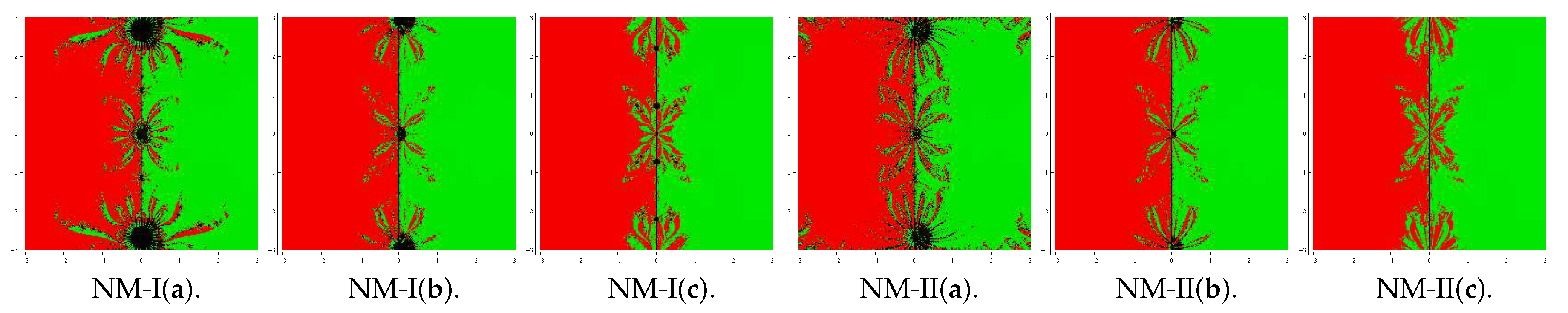
To start with we take the initial point in a rectangular region that contains all the roots of a polynomial The iterative method when starts from point in a rectangle either converges to the root or eventually diverges. The stopping criterion for convergence is considered to be up to a maximum of 25 iterations. If the required accuracy is not achieved in 25 iterations, we conclude that the method with initial point does not converge to any root. The strategy adopted is as follows: A color is allocated to each initial point lying in the basin of attraction of a root. If the iteration initiating at converges, it represents the attraction basin painted with assigned color to it, otherwise, the non-convergent cases are painted by the black color.
To view the geometry in complex plane, we characterize attraction basins associated with the methods NM-I(a–c) and NM-II(a–c) considering the following four polynomials:
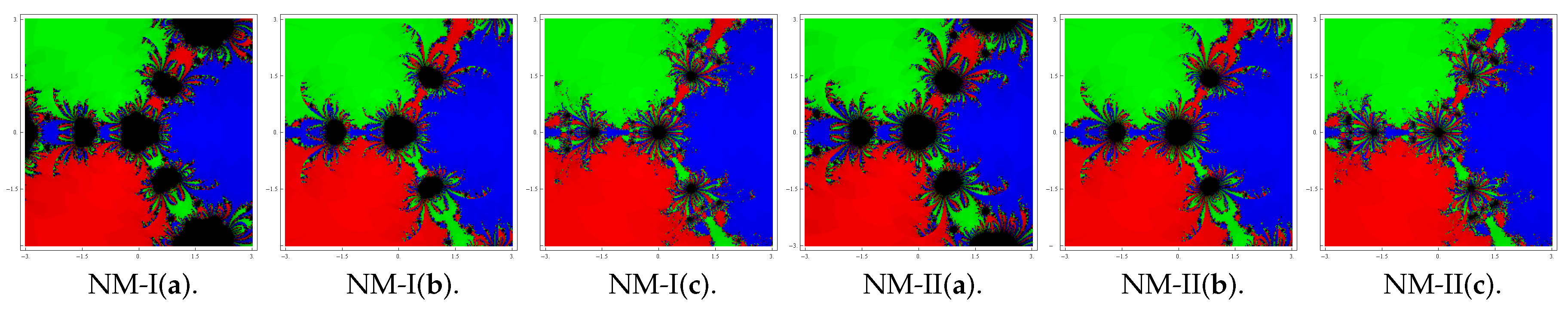
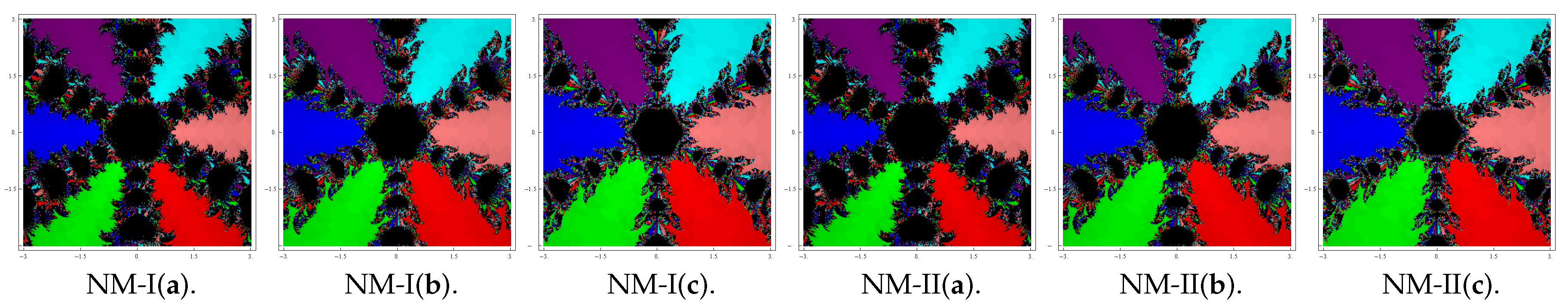
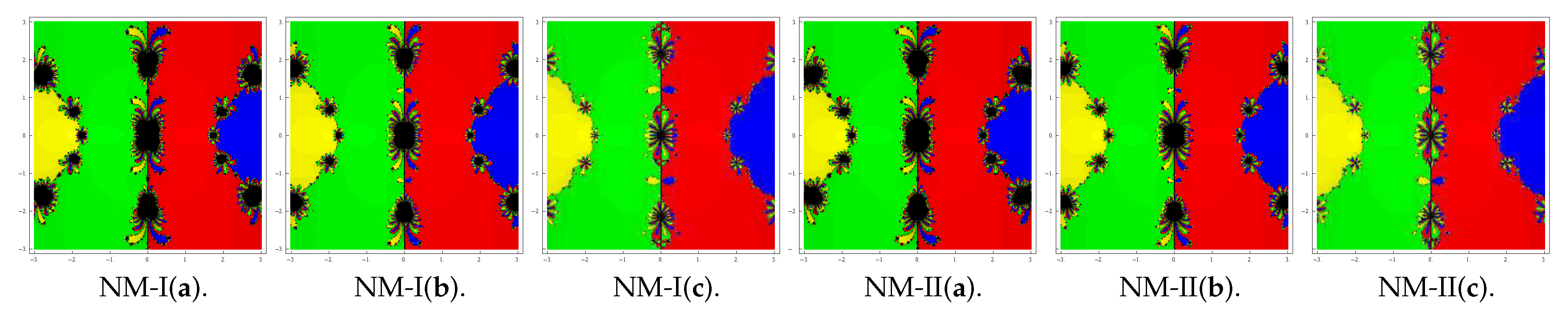
Problem 1. Consider the polynomial , which has roots with multiplicity three. We use a grid of points in a rectangle of size and assign red color to each initial point in the attraction basin of root and green color to each point in the attraction basin of root 1. The basins so plotted for NM-I(a–c) and NM-II(a–c) are displayed in Figure 1. Looking at these graphics, we conclude that the method NM-II(c) possesses better stability followed by NM-I(c) and NM-II(b). Black zones in the figures show the divergent nature of a method when it starts assuming initial point from such zones. Problem 2. Let that has three roots each with multiplicity two. To plot the graphics, we use a grid of points in a rectangle of size and assign the colors blue, green and red corresponding to each point in the basins of attraction of 1, and . Basins drawn for the methods NM-I(a–c) and NM-II(a–c) are shown in Figure 2. As can be observed from the pictures, the method NM-I(c) and NM-II(c) possess a small number of divergent points and therefore have better convergence than the remaining methods. Problem 3. Let with six roots each with multiplicity . Basins obtained for the considered methods are presented in Figure 3. To draw the pictures, the red, blue, green, pink, cyan and magenta colors have been assigned to the attraction basins of the six roots. We observe from the graphics that the method NM-I(c) and NM-II(c) have better convergence behavior since they have lesser number of divergent points. On the other hand NM-I(a) and NM-II(a) contain large black regions followed by NM-I(b) and NM-II(b) indicating that the methods do not converge in 25 iterations starting at those points. Problem 4. Consider the polynomial that has four simple roots . In this case also, we use a grid of points in a rectangle of size and allocate the red, blue, green and yellow colors to the basins of attraction of these four roots. Basins obtained for the methods are shown in Figure 4. Observing the basins, we conclude that the method NM-II(c) possesses better stability followed by NM-I(c). Remaining methods show chaotic nature along the boundaries of the attraction basins. Looking at the graphics, one can easily judge the stable behavior and so the better convergence of any method. We reach to a root, if we start the iteration choosing anywhere in the basin of that root. However, if we choose an initial guess in a region wherein different basins of attraction meet each other, it is difficult to predict which root is going to be attained by the iterative method that starts from . So, the choice of in such a region is not a good one. Both black regions and the regions with different colors are not suitable to assume the initial guess as when we are required to achieve a particular root. The most intricate geometry is between the basins of attraction, which corresponds to the cases where the method is more demanding with respect to the initial point. From the basins, one can conclude that the method NM-II(c) possesses better stability followed by NM-I(c) than the remaining methods.
4. Numerical Tests
In this section, we apply the special cases NM-i(j), i = I, II and j = a, b, c of the scheme (
4), corresponding to the combinations of
: cases 1 and 2 with that of
): cases 5, 6 and 7, to solve some nonlinear equations for validation of the theoretical results that we have derived. The theoretical seventh order of convergence is verified by calculating the computational order of convergence (COC)
which is given in (see [
28]). Comparison of performance is also done with some existing methods such as the sixth order methods by Geum et al. [
22,
23], which are already expressed by (
2) and (
3). To represent
, we choose the following four special cases in the formula (
2) and denote the respective methods by GKN-I(j), j = a, b, c, d:
- (a)
- (b)
- (c)
where , , , .
- (d)
where , ,
, .
For the formula (
3), considering the following four combinations of the functions
and
, and denoting the corresponding methods by GKN-II(j), j = a, b, c, d:
- (a)
, .
- (b)
, .
- (c)
, .
- (d)
, .
Computational work is compiled in the programming package of Mathematica software using multiple-precision arithmetic. Numerical results as displayed in
Table 1,
Table 2,
Table 3,
Table 4 and
Table 5 contain: (i) number of iterations
needed to converge to desired solution, (ii) last three successive errors
, (iii) computational order of convergence (COC) and (iv) CPU-time (CPU-t) in seconds elapsed during the execution of a program. Required iteration
and elapsed CPU-time are computed by selecting
as the stopping condition.
For numerical tests we select seven problems. The first four problems are of practical interest where as last three are of academic interest. In the problems we need not to calculate the root multiplicity m and it is set a priori, before running the algorithm.
Example 1 (Eigen value problem)
. Finding Eigen values of a large sparse square matrix is a challenging task in applied mathematics and engineering sciences. Calculating the roots of a characteristic equation of matrix of order larger than 4 is even a big job. We consider the following 9 × 9 matrix.
We calculate the characteristic polynomial of the matrix
as
This function has a multiple root
with multiplicity 4. We select initial value
and obtain the numerical results as shown in
Table 1.
Example 2 (Manning equation for fluid dynamics)
. Next, the problem of isentropic supersonic flow around a sharp expansion corner is chosen (see [2]). Relation among the Mach number before the corner (say ) and after the corner (say ) is given bywhere and γ is the specific heat ratio of gas. For a specific case, the above equation is solved for for , given that , and . Then, we have thatwhere . Let us consider this particular case seven times using same values of the involved parameters and then obtain the nonlinear function The above function has one root at of multiplicity 7 with initial approximations . Computed numerical results are shown in Table 2. Example 3 (Beam designing model)
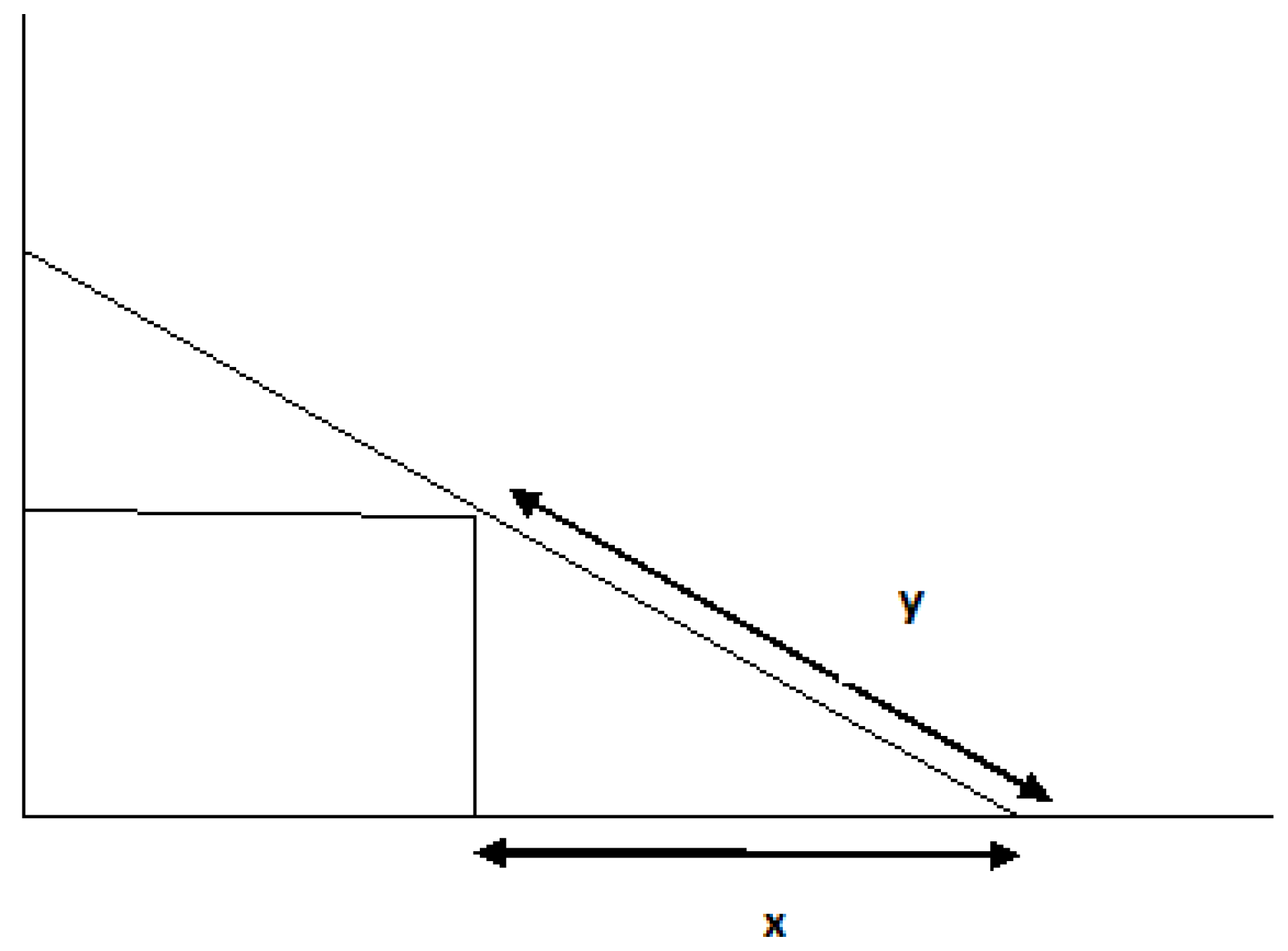
. We consider the problem of beam positioning (see [4]) where a beam of length r unit leans against the edge of a cubical box of sides 1 unit distance each, such that one end of the beam touches the wall and the other end touches the floor, as depicted in Figure 5. The problem is: What will be the distance alongside the floor from the base of wall to the bottom of beam? Suppose that
y is distance along the beam from the floor to the edge of the box and
x is the distance from the bottom of box to the bottom of beam. For a given
r, we can obtain the equation
One of the roots of this equation is the double root
. We select the initial guess
to find the root. Numerical results by various methods are shown in
Table 3.
Example 4 (van der Waals equation)
. Consider the Van der Waals equationthat describes nature of a real gas by adding in the ideal gas equation two parameters, and , which are specific for each gas. To find the volume V in terms of rest of the parameters one requires to solve the equation Given a set of values of and of a particular gas, one can find values for n, P and T, so that this equation has three real roots. Using a particular set of values (see [3]), we have the equationwhere . This equation has a multiple root with multiplicity 2. The initial guess chosen to obtain the root 1.75 is . Numerical results are shown in Table 4. Example 5. Consider now the standard nonlinear test function (see [23]) The root of multiplicity 2 is computed with initial guess . Numerical results are displayed in Table 5. Example 6. Let us assume another nonlinear test function given as (see [22]) The root of this function is of multiplicity 5. This root is calculated assuming the initial approximation . Results so obtained are shown in Table 6. Example 7. Lastly, consider the test function The function has multiple root of multiplicity 4. We choose the initial approximations for obtaining the root of the function. The results computed by various methods are shown in Table 7. From the numerical values of errors we observe the increasing accuracy in the values of successive approximations as the iteration proceed, which points to the stable nature of the methods. Like the existing methods, the convergence behavior of new methods is also consistent. At the stage when stopping criterion has been satisfied we display the value ‘0’ of . From the calculation of computational order of convergence shown in the penultimate column in each table, we verify the theoretical convergence of seventh order. The entries of last column in each table show that the new methods consume less CPU-time during the execution of program than the time taken by existing methods. This confirms the computationally more efficient nature of the new methods. Among the new methods, the better performers (in terms of accuracy) are NM-I(c) and NM-II(c) since they produce approximations of the root with small error. However, this is not true when execution time is taken into account because if one method is better in some situations, then the other is better in some other situation. The main purpose of implementing the new methods for solving different type of nonlinear equations is purely to illustrate the better accuracy of the computed solution and the better computational efficiency than existing techniques. Similar numerical experimentation, performed on a variety of numerical problems of different kinds, confirmed the above remarks to a large extent.


