Article

Cosmological Consequences of a Parametrized Equation of State

1
Department of Mathematics, COMSATS University Islamabad Lahore-Campus, Lahore-54000, Pakistan
2
Division of Human Support System, Faculty of Symbiotic Systems Science, Fukushima University, Fukushima 960-1296, Japan
3
Department of Statistics, COMSATS University Islamabad, Lahore-Campus, Lahore-54000, Pakistan
*
Author to whom correspondence should be addressed.
Symmetry 2019, 11(8), 1009; https://doi.org/10.3390/sym11081009
Submission received: 24 May 2019 / Revised: 9 July 2019 / Accepted: 16 July 2019 / Published: 5 August 2019
(This article belongs to the Special Issue Cosmological Inflation, Dark Matter and Dark Energy)

Abstract

:
We explore the cosmic evolution of the accelerating universe in the framework of dynamical Chern–Simons modified gravity in an interacting scenario by taking the flat homogeneous and isotropic model. For this purpose, we take some parametrizations of the equation of state parameter. This parametrization may be a Taylor series extension in the redshift, a Taylor series extension in the scale factor or any other general parametrization of ω . We analyze the interaction term which calculates the action of interaction between dark matter and dark energy. We explore various cosmological parameters such as deceleration parameter, squared speed of sound, Om-diagnostic and statefinder via graphical behavior.

1. Introduction

It is believed that in present day cosmology, one of the most important discoveries is the acceleration of the cosmic expansion [1,2,3,4,5,6,7,8,9,10]. It is observed that the universe expands with repulsive force and is not slowing down under normal gravity. This unknown force, called dark energy (DE), and is responsible for current cosmic acceleration. In physical cosmology and astronomy, DE is a mysterious procedure of energy which is assumed to pervade all of space which tends to blast the extension of the universe. However, the nature of DE is still unknown which requires further attention [11] (for recent reviews on the so-called geometric DE, i.e., modified gravity theories to explain the late-time cosmic acceleration, see, for example [12,13,14,15,16,17]). In the standard Λ -cold dark matter (CDM) model of cosmology, the whole mass energy of the cosmos includes 4.9% of usual matter, 26.8% of DM and 68.3% of a mysterious form of energy recognized as dark energy. In astrophysics, DM is an unknown form of matter which appears only participating in gravitational interaction, but does not emit nor absorb light [18]. The nature of DM is still unknown, but its existence is proved by astrophysical observations [19]. The majority of DM is thought to be non-baryonic in nature [20].
In order to explain DE, a large number of models have been suggested such as quintessence [21], quintom [22,23,24], Chaplygin gas with its modified model [25,26,27], K-essence [28,29,30], new agegraphic DE [31,32], holographic DE model [33,34,35], pilgrim DE model [36,37,38], Tsallis holographic DE (THDE) [39]. Among all of these, the simplest is the cosmological constant model and this model is compatible with observations [1]. In the cosmological framework, the equation of state (EoS) parameter, ω , gives the relation among energy density and pressure [40]. This is a dimensionless parameter and descrbes the phases of the cosmos [41]. The EoS parameter might be used in Friedmann–Robertson–Walker (FRW)’ equations to define the evolution of an isotropic universe filled with a perfect fluid. The EoS parameter governs not only the gravitational properties of DE but also its evolution. The EoS parameter may be a constant or a time dependent function [1]. It is observed that this parameter gives constant ranges by using various observational schemes. For deviating DE, a parametrized formation of ω is supposed. Parametrization may be a Taylor series extension in the redshift, a Taylor series extension in the scale factor or any other parametrization of ω [42,43,44,45,46,47,48,49,50,51,52,53,54,55,56]. Using different considerations of parametrization, the cosmological parameters can be constrained [57,58,59].
On the other hand, different modified theories of gravity have been proposed in order to explain cosmic acceleration. The dynamical Chern–Simons modified gravity has been recently proposed [60] which is motivated from string theory and loop quantum gravity [61,62]. In this gravity, Jawad and Rani [63] investigated various cosmological parameters and planes for pilgrim DE models in that FRW universe. Jawad and Sohail [62] explored different cosmological planes as well as parameters for modified DE. Till now, various works have been done on the investigation of cosmic expansion scenario with different cosmological parameters [64,65,66,67,68,69,70,71]. In the present work, we use the constructed models in the frame work of dynamical Chern–Simons modified gravity and investigate the different cosmological parameters such as the deceleration parameter, squared speed of sound, state finder parameters and Om-diagnostic.
This paper is organized as follows: in the next section, we provide the basic cosmological scenario of dynamical Chern–Simons modified gravity and construct the field equations in for flat FRW spacetime. We take interaction scenario for constitutes DE and DM with the help of conservation equations. The holographic DE (HDE) density is used as DE model with Hubble horizon as IR cut-off. In Section 3, we provide the parametrization model of EoS parameter and construct the setup to discuss the cosmic evolution of the universe. Also, we analyze the interaction term for the corresponding parametrizations. In Section 4, we discuss the cosmological parameters such as deceleration, squared speed of sound, Om-diagnostic and statefinder. Last section comprises the results.

2. Dynamical Chern–Simons Modified Gravity

In this section, we describe the dynamical Chern–Simons modified gravity by the following action
S = 1 16 π G V d 4 x [ g R + l 4 * R ρ σ μ ν R ρ σ μ ν θ 1 2 g μ ν μ θ ν θ + V ( θ ) ] + S m a t ,
here R is the Ricci scalar, * R ρ σ μ ν R ρ σ μ ν is the topological invariant called the pontryagin term, l is the coupling constant, θ is the dynamical variable, S m a t is the action of matter and V ( θ ) is the potential. Now in case of string theory, we take V ( θ ) = 0 . The variation of Equation (1) corresponding to metric g μ ν and scalar field θ , respectively, give the following field equations
G μ ν + l C μ ν = 8 π G T μ ν ,
g μ ν μ ν θ = l 64 π * R ρ σ μ ν R ρ σ μ ν ,
where G μ ν is known as Einstein tensor and C μ ν appears as Cotton tensor which is defined as
C μ ν = 1 2 g ( ( ρ θ ) ε ( ρ β τ τ μ R β ν ) + ( σ ρ θ ) * R ρ ( μ ν ) σ .
The energy–momentum tensor related to scalar field and matter are given by
T ^ μ ν θ = μ θ ν θ 1 2 g μ ν ρ θ ρ θ ,
T μ ν = ( ρ + p ) u μ u ν + p g μ ν ,
here T ^ μ ν θ shows the scalar field contribution and T μ ν represents the matter contribution while p and ρ indicate the pressure and energy density respectively. Also, u μ = ( 1 , 0 , 0 , 0 ) is the four velocity. In case of flat FRW universe, first Friedmann equation for dynamical Chern–Simons modified gravity becomes
H 2 = 1 3 ( ρ m + ρ d ) + 1 6 θ ˙ 2 ,
where H = a ˙ a represents the Hubble parameter, a is the scale factor and dot indicates the derivative with respect to cosmic time, ρ = ρ m + ρ d is the effective density and 8 π G = 1 . We assume p m = 0 then for ordinary matter, the conservation equations are given as
ρ ˙ m + 3 H ρ m = 0 ,
ρ ˙ d + 3 H ( ρ d + p d ) = 0 .
For FRW universe the pontryagin term vanishes, so the scalar field in Equation (3) reduces to the following form
g μ ν μ ν θ = g μ ν ( ν μ θ ) = 0 .
By taking θ = θ ( t ) , we get the following equation
θ ¨ + 3 H θ ˙ = 0 .
The solution of this equation for θ ˙ is θ ˙ = b a 3 where b is an integration constant. Using this solution in Equation (6), we have
H 2 = 1 3 ( ρ m + ρ d ) + 1 6 b 2 a 6 .
Taking into account the equation of continuity Equation (8), Equation (12) takes the form
2 H ˙ 3 H 2 1 6 b 2 a 6 = p d .
Equation (12) can be re-written as
E 2 ( z ) = 1 3 H 0 2 ( ρ m + ρ d ) + 1 6 H 0 2 b 2 a 6 ,
where E ( z ) = H H 0 is a normalized Hubble parameter, z is the redshift function which is defined as 1 + z = a 0 a . Interaction is an idea of two way action that occur when two or more objects have effect on each other. The continuity equations for energy densities are defined as
ρ m 3 1 + z ρ m = Q H 0 E ( z ) ( 1 + z ) ,
ρ d 3 1 + ω d 1 + z ρ d = Q H o E ( z ) ( 1 + z ) .
Here, prime denotes the derivative with respect to the redshift and Q is the interaction term which calculates the action of interaction between the DM and DE. Basically, Q tells about the rate of energy exchange between DM and DE. When Q > 0 , it means that energy is being converted from DE to DM. For Q < 0 , the energy is being converted from DM to DE [72]. In the preceding prospectus of DE, HDE is one of the sensational attempts to analyze the nature of DE in the frame of quantum gravity. The HDE is based on holographic principle which states that all information relevant to a physical system inside a spatial region can be observed on its boundary instead of its volume. The relation of ultra-violet UV ( Λ ) and infra-red IR ( L ) is introduced by Cohen et al. [73] which plays a key role in the construction of HDE model [74]. The relation is about the energy of vacuum of a system with particular size whose maximal quantity should not be greater than the black hole mass of the similar size. This can be indicated as L 3 ρ d L M p 2 , here M p 2 = ( 8 π G ) 1 and L represents the reduced Planck mass and IR cutoff respectively [75]. From the above inequalities, the HDE density takes the following form
ρ d = 3 c 2 H 0 2 E 2 ( z ) ,
where c is the constant parameter of the dimensionless HDE and describes the expansion of universe and it lies in the interval 0 < c 2 < 1 and L is taken as Hubble horizon. By inserting Equations (15)–(17) in (14) we get the following expression
ω d = ( 1 + z ) d E 2 ( z ) 3 c 2 E 2 ( z ) d z b 2 ( 1 + z ) 6 6 c 2 H 0 2 E 2 ( z ) 1 c 2 ,
after some calculation we get the following result
d E 2 ( z ) d z ( 3 + 3 c 2 ω d ) E 2 ( z ) 1 + z = b 2 ( 1 + z ) 5 2 H 0 2 .

3. Parametrizations of Equation of State Parameter

Parametrization is a process of choosing different parameters and is used for the comparison of two datasets. In cosmological context, the EoS parameter is the relation between energy density and pressure and it helps to classify the accelerated and decelerated phases of the universe. At ω = 0 , this parameter corresponds to non-relativistic matter and involves the radiation era 0 < ω < 1 3 for the accelerated phase of the universe. At ω < 1 , ω = 1 and 1 < ω < 1 3 it represents the phantom, cosmological constant and quintessence eras respectively. A parametrized formation of ω is assumed for deviating DE. We construct two different models; one with a constant EoS parameter and other with a dark fluid in the existence of DM [1,76]. By using a function of redshift the variation of EoS parameter can be estimated and many parametrizations have been suggested so far. We use the following parametrizations
ω 1 d = ω 0 ,
ω 2 d = ω 0 + ω 1 q .
At present, ω 0 is the value of EoS parameter, ω 1 is the parameter of the model that is determined by using the observational data [76] and q is the deceleration parameter. By inserting Equation (20) in (19), we have
E 2 ( z ) = b 2 ( 1 + z ) 6 2 H 0 2 ( 3 3 c 2 ω 0 ) + A ( 1 + z ) 3 + 3 c 2 ω 0 ,
where A is a constant of integration. Similarly by inserting Equation (21) in (19), we get the following result
E 2 ( z ) = b 2 2 H 0 2 ( 3 3 c 2 ω 0 8 c 2 ω 1 1 3 2 ( c 2 ω 1 ) ) ( 1 + z ) 6 11 c 2 ω 1 1 3 2 ( c 2 ω 1 ) + B ( 1 + z ) 3 + 3 c 2 ω 0 3 c 2 ω 1 1 3 2 ( c 2 ω 1 ) .
Now, we analyze the interaction term Q for the chosen parametrization of EoS parameter. Using Equations (14) and (17), we obtain the energy density of DM in the following form
ρ m = 3 H 0 2 E 2 ( z ) ( 1 c 2 ) b 2 2 ( 1 + z ) 6 .
Taking the derivative with respect to z of Equation (24) along with ρ m in the continuity equation related to DM, we have
( 1 + z ) d d z ln ( E 2 ( z ) ) = 3 + b 2 ( 1 + z ) 6 2 H 0 2 E 2 ( z ) ( 1 c 2 ) Q 3 H 0 3 E 3 ( z ) ( 1 c 2 ) .
Using Equations (14)–(16), we get the following result
( 1 + z ) 3 d d z ln ( E 2 ( z ) ) = 1 + ω d 1 + r + b 2 ( 1 + z ) 6 2 b 2 ( 1 + z ) 6 2 H 0 2 E 2 ( z ) ,
where r is the coincidence parameter which is defined as r = ρ m ρ d with the help of Equations (17) and (24). Comparing the above equations, it yields
Q 9 H 0 3 E 3 ( z ) ( 1 c 2 ) = ω d 1 + r + b 2 ( 1 + z ) 6 2 + b 2 ( 1 + z ) 6 2 H 0 2 E 2 ( z ) 1 + 1 3 ( 1 c 2 ) .
At present time, the above equation becomes
Q 0 = 9 ( 1 c 2 ) ω d , 0 1 + r 0 + b 2 2 + 9 b 2 ( 1 c 2 ) 2 1 + 1 3 ( 1 c 2 ) .
It is significant to express that the value of Q-term predicts the rate at which the universe expands and coincidence parameter decreases. Using the positivity condition of the Q-term at present time, Equation (28) takes the following form
ω d , 0 < ( 1 + r + b 2 2 ) 3 b 2 ( 1 c 2 ) + b 2 b ( 1 c 2 ) .
The normalized Hubble parameter in terms of coincidence parameter is obtained by the ratio of Equations (17) and (24) such that
E 2 ( z ) = b 2 ( 1 + z ) 6 6 H 0 2 c 2 ( r ( z ) r c ) ,
where r c = ( 1 c 2 ) ( c 2 ) is a constant quantity. This parameter shows the singular behavior at r ( z ) = r c . At present time, r c = r o + b 2 6 1 b 2 6 , where c 2 = 1 b 2 6 1 + r 0 . For the coincidence parameter, we can consider a CPL-type parametrization form [42] r ( z ) = r o + ϵ o z 1 + z , where ϵ o = r o . We can notice that above parametrization becomes singular at z = 1 and it has a linear behavior and bounded nature for low and high value of redshift respectively. Taking into account the above parametrization, we get the value of redshift z s , such that z s = r o r c ϵ o ( 1 + ( r o r c ) ϵ o ) . For the singular behavior, we have the condition 1 < z s < 0 . After some manipulation, we obtain
r ( z ) r c = ϵ o ( z z s ) ( 1 + z s ) ( 1 + z ) 0 z z s ,
which yields ( ϵ o z s ) ( 1 + z s ) 0 at present time. Substituting these results in Equation (31), it can be written as
E 2 ( z ) = η b 2 ( 1 + z ) 7 6 H 0 2 ( z z s ) ,
here η : = ( 1 + z s ) c 2 ϵ o > 0 since ϵ o > 0 . Moreover, we define the function θ ( z ) : = ( 1 + z ) ( z z s ) and substitute Equation (32) in (26), we get the following result
1 + ω d 1 + r + b 2 ( 1 + z ) 6 2 = 9 + η θ ( 7 + θ ) 3 η θ .
Using above result the expression (27) for the Q-term can be written as
Q 9 H 0 3 E 3 ( z ) = ( 1 c 2 ) 9 η θ ( 4 + θ ) 3 η θ + b 2 ( 1 + z ) 6 ( 1 c 2 ) 2 H 0 2 E 2 ( z ) + b 2 ( 1 + z ) 6 6 H 0 2 E 2 ( z ) .
For ω 1 d the expression for the Q-term takes the following form
Q 1 = 9 H 0 3 b 2 ( 1 + z ) 6 2 H 0 2 ( 3 3 c 2 ω 0 ) + A ( 1 + z ) 3 + 3 c 2 ω 0 3 2 ( 1 c 2 ) × ( ω 0 1 + r o + ϵ o z 1 + z + b 2 ( 1 + z ) 6 2 + b 2 ( 1 + z ) 6 2 H 0 2 ( b 2 ( 1 + z ) 6 2 H 0 2 ( 3 3 c 2 ω 0 ) + A ( 1 + z ) 3 + 3 c 2 ω 0 ) × 1 + 1 3 ( 1 c 2 ) ) .
Similarly for ω 2 d , the Q-term is reduced in the following relation
Q 2 = b 2 2 H 0 2 ( 3 3 c 2 ω 0 8 c 2 ω 1 1 3 2 ( c 2 ω 1 ) ) ( 1 + z ) 6 11 c 2 ω 1 1 3 2 ( c 2 ω 1 ) + B ( 1 + z ) 3 + 3 c 2 ω 0 3 c 2 ω 1 1 3 2 ( c 2 ω 1 ) 3 2 × 9 H 0 3 ( 1 c 2 ) ( ω 0 + ω 1 q 1 + r o + ϵ o z 1 + z + b 2 ( 1 + z ) 6 2 1 + 1 3 ( 1 c 2 ) + b 2 ( 1 + z ) 6 2 H 0 2 ( b 2 2 H 0 2 ( 3 3 c 2 ω 0 8 c 2 ω 1 1 3 2 ( c 2 ω 1 ) ) ( 1 + z ) 6 11 c 2 ω 1 1 3 2 ( c 2 ω 1 ) + B ( 1 + z ) 3 + 3 c 2 ω 0 3 c 2 ω 1 1 3 2 ( c 2 ω 1 ) ) ) .
In Figure 1, the plot of Q 1 as a function of z is expressed for three different values of ω 0 = 0 . 8 , 0 . 9 , 1 . The specific values for the other constants are b = 3 , H 0 = 67 , c = 0 . 8 , A = 0 . 002 , ϵ o = 0 . 1 and r o = 0 . 43 . We can observe that Q 1 inclines the positive trajectory. It is mentioned [77] that the interaction term must not change its sign during cosmic evolution and is observationally verified. The plot of Q 2 versus z for ω 2 d as shown in Figure 2. The particular values of other constants are ω 1 = 0 . 2 , 0 . 5 , 0 . 8 , B = 0 . 002 and remaining are same as in the above case. It can be seen that Q 2 gives the positive behavior for all epochs related to z.

4. Cosmological Parameters

In this section, we construct some cosmological parameters such as the deceleration parameter, stability analysis, statefinder and Om-diagnostic corresponding to parametrizations of EoS parameter in the presence of dynamical Chern–Simons modified gravity.

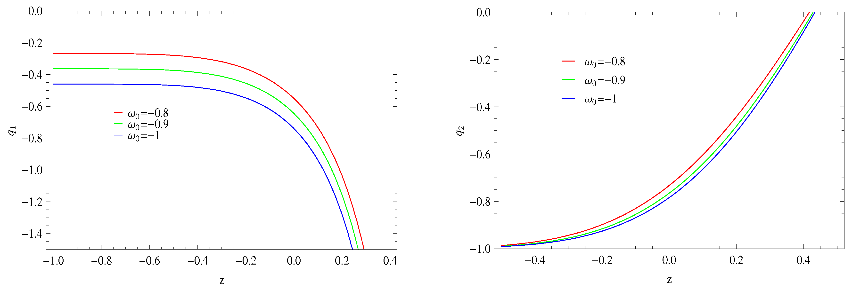
4.1. Deceleration Parameter

The deceleration parameter can be described as follows
q = 1 H ˙ H 2 .
This parameter characterizes the accelerated as well as decelerated phases of the universe. For q [ 1 , 0 ) , it shows the accelerated phase of the universe and q 0 exhibits the decelerated phase of the universe. The time derivative of Hubble parameter gives the following relation in terms of redshift function
H ˙ H 2 = ( 1 + z ) E d E d z .
Inserting Equation (38) into (37), we have
q = 1 + ( 1 + z ) E d E d z .
The deceleration parameter for ω 1 d can be evaluated by using Equations (22) and (39) such that
q 1 = 1 + ( 1 + z ) 2 ( b 2 ( 1 + z ) 6 2 H 0 2 ( 3 3 c 2 ω 0 ) + A ( 1 + z ) 3 + 3 c 2 ω 0 ) × 3 b 2 ( 1 + z ) 5 H 0 2 ( 3 3 c 2 ω 0 ) + A ( 1 + z ) 2 + 3 c 2 ω 0 ( 3 + 3 c 2 ω 0 ) .
The plot of this equation in shown in Figure 3 (left) versus z for three different values of ω 0 . The particular values of other constants are same as in above case. For z > 0 , the deceleration parameter transits towards the range for accelerated phase. For present and future epochs, this parameter represents the accelerated phase of the evolving universe. Substituting the Equation (23) into (39), the expression of deceleration parameter for ω 2 d takes the following form
q 2 = 1 + ( 1 + z ) b 2 ( 1 + z ) 6 11 c 2 ω 1 1 3 2 ( c 2 ω 1 ) H 0 2 ( 3 3 c 2 ω 0 8 c 2 ω 1 1 3 2 ( c 2 ω 1 ) ) + 2 B ( 1 + z ) 3 + 3 c 2 ω 0 3 c 2 ω 1 1 3 2 ( c 2 ω 1 ) 1 × [ ( 3 3 c 2 ω 1 + 3 c 2 ω 0 ) B ( 1 + z ) 1 + 3 3 c 2 ω 1 + 3 c 2 ω 0 1 3 2 ( c 2 ω 1 ) 1 3 2 ( c 2 ω 1 ) + 6 11 c 2 ω 1 1 3 2 c 2 ω 1 × b 2 ( 1 + z ) 1 + 6 11 c 2 ω 1 1 3 2 ( c 2 ω 1 ) 2 H 0 2 3 8 c 2 ω 1 1 3 2 ( c 2 ω 1 ) 3 c 2 ω 0 ] .
For ω 2 d , we plot the deceleration parameter q 2 as shown in Figure 3 (right) for same parametric values. In this scenario, the deceleration parameter exhibits accelerated phase of the universe since it remains between −1 and 0 for all values of ( ω 0 , ω 1 ) .

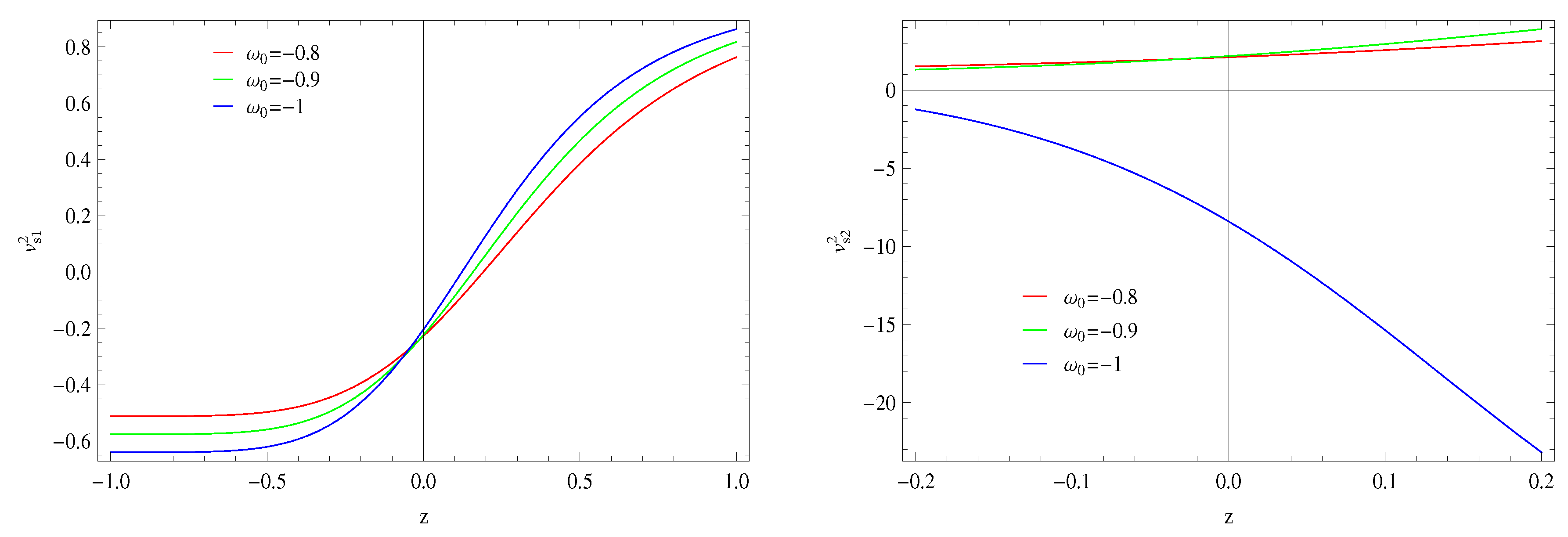
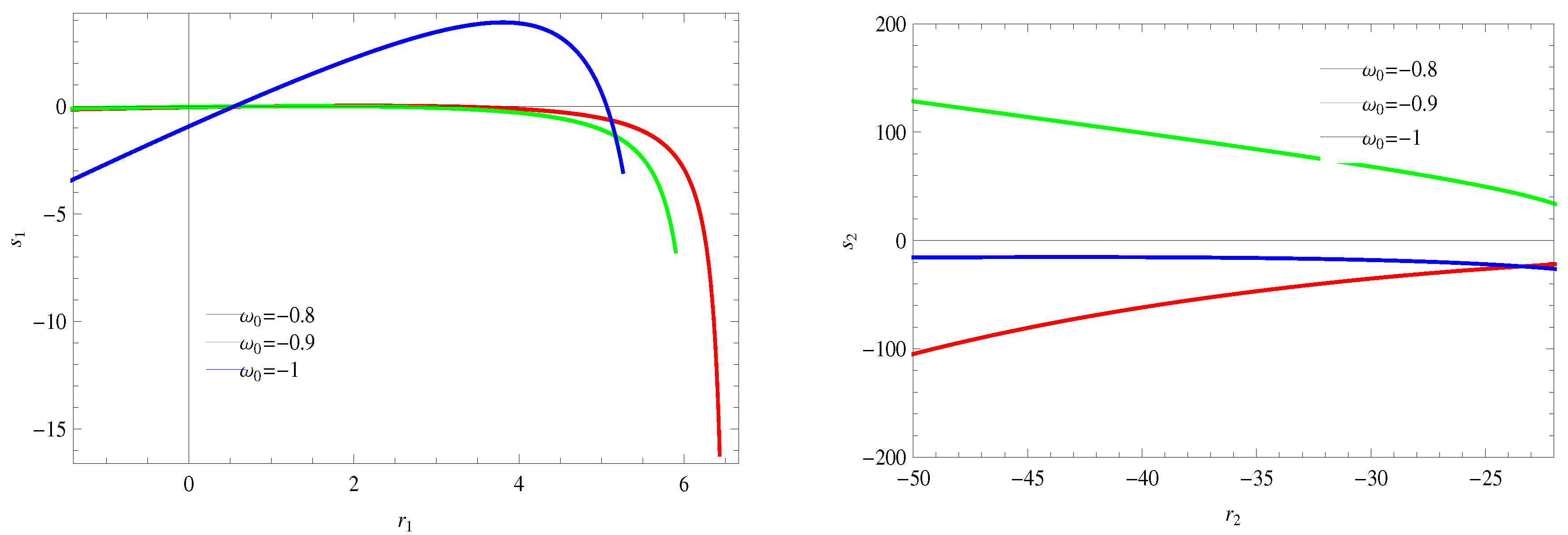
4.2. Stability Analysis

The squared speed of sound can be described as follows
v s 2 = d p d ρ .
The squared speed of sound parameter is used to discuss the stability of model. That is, v s 2 < 0 leads to the unstable behavior of the model while v s 2 0 corresponds to the stable behavior. Inserting Equations (12), (13) and (22) in (42), we obtain the squared speed of sound for ω 1 d as follows
v s 1 2 = ( 3 b 2 ( 1 + z ) 5 + H 0 2 ( 1 + z ) ( 15 b 2 ( 1 + z ) 4 H 0 2 ( 3 3 c 2 ω 0 ) + A ( 1 + z ) 1 + 3 c 2 ω 0 × ( 2 + 3 c 2 ω 0 ) ( 3 + 3 c 2 ω 0 ) ) 2 H 0 2 ( 3 b 2 ( 1 + z ) 5 H 0 2 ( 3 3 c 2 ω 0 ) + A ( 1 + z ) 2 + 3 c 2 ω 0 + ( 3 + 3 c 2 ω 0 ) ) ) 3 A H 0 2 ( 1 + z ) 2 + 3 c 2 ω 0 ( 3 + 3 c 2 ω 0 ) + 3 b 2 ( 1 + z ) 5 c 2 ω 0 1 c 2 ω 0 1 .
Taking into account Equations (12), (13) and (23) in (42), the relation of squared speed of sound for ω 2 d takes the following form
v s 2 2 = [ 3 b 2 ( 1 + z ) 5 + 3 b 2 ( 1 + z ) 5 11 c 2 ω 1 1 3 2 c 2 ω 1 ( 6 11 c 2 ω 1 1 3 2 c 2 ω 1 ) 2 ( 3 3 c 2 ω 0 8 c 2 ω 1 1 3 2 c 2 ω 1 ) + 3 B H 0 2 × ( 1 + z ) 2 + 3 c 2 ω 1 3 c 2 ω 1 1 3 2 c 2 ω 1 ( 3 + 3 c 2 ω 1 3 c 2 ω 1 1 3 2 c 2 ω 1 ) ] 1 [ b 2 2 ( 1 + z ) 6 3 B H 0 2 ( 1 + z ) 3 + 3 c 2 ω 1 3 c 2 ω 1 1 3 2 c 2 ω 1 3 b 2 ( 1 + z ) 6 11 c 2 ω 1 1 3 2 c 2 ω 1 2 ( 3 3 c 2 ω 0 8 c 2 ω 1 1 3 2 c 2 ω 1 ) + b 2 ( 1 + z ) 6 11 c 2 ω 1 1 3 2 c 2 ω 1 ( 6 11 c 2 ω 1 1 3 2 c 2 ω 1 ) ( 3 3 c 2 ω 0 8 c 2 ω 1 1 3 2 c 2 ω 1 ) + 2 B H 0 2 ( 1 + z ) 3 + 3 c 2 ω 1 3 c 2 ω 1 1 3 2 c 2 ω 1 × ( 3 + 3 c 2 ω 1 3 c 2 ω 1 1 3 2 c 2 ω 1 ) b 2 ( 1 + z ) 5 11 c 2 ω 1 1 3 2 c 2 ω 1 ( 6 11 c 2 ω 1 1 3 2 c 2 ω 1 ) 2 ( 3 3 c 2 ω 0 8 c 2 ω 1 1 3 2 c 2 ω 1 ) H 0 2 B ( 1 + z ) 2 + 3 c 2 ω 1 3 c 2 ω 1 1 3 2 c 2 ω 1 ( 3 + 3 c 2 ω 1 3 c 2 ω 1 1 3 2 c 2 ω 1 ) 3 b 2 ( 1 + z ) 5 + b 2 ( 1 + z ) 5 11 c 2 ω 1 1 3 2 c 2 ω 1 ( 5 11 c 2 ω 1 1 3 2 c 2 ω 1 ) ( 6 11 c 2 ω 1 1 3 2 c 2 ω 1 ) ( 3 3 c 2 ω 0 8 c 2 ω 1 1 3 2 c 2 ω 1 ) + 2 B H 0 2 × ( 1 + z ) 2 + 3 c 2 ω 1 3 c 2 ω 1 1 3 2 c 2 ω 1 ( 2 + 3 c 2 ω 1 3 c 2 ω 1 1 3 2 c 2 ω 1 ) × ( 3 + 3 c 2 ω 1 3 c 2 ω 1 1 3 2 c 2 ω 1 ) ] .
The plot of v s 1 2 is expressed in Figure 4 (left). It can be seen that the trajectories of squared speed of sound show positive behavior for a positive range of z (except some values) which gives the stability of the model. However, for a small range of positive values of z , z = 0 and z < 0 , the model expresses unstable behavior. In Figure 4 (right), the graph of squared speed of sound versus redshift parameter is given. The trajectories for ω 0 = 0 . 8 , 0 . 9 give the positive behavior for all values of z while for ω 0 = 1 , the squared speed of sound represents negative behavior for all values. This shows the stable behavior in first case while in latter case, the model is unstable.

4.3. Statefinder Parameters
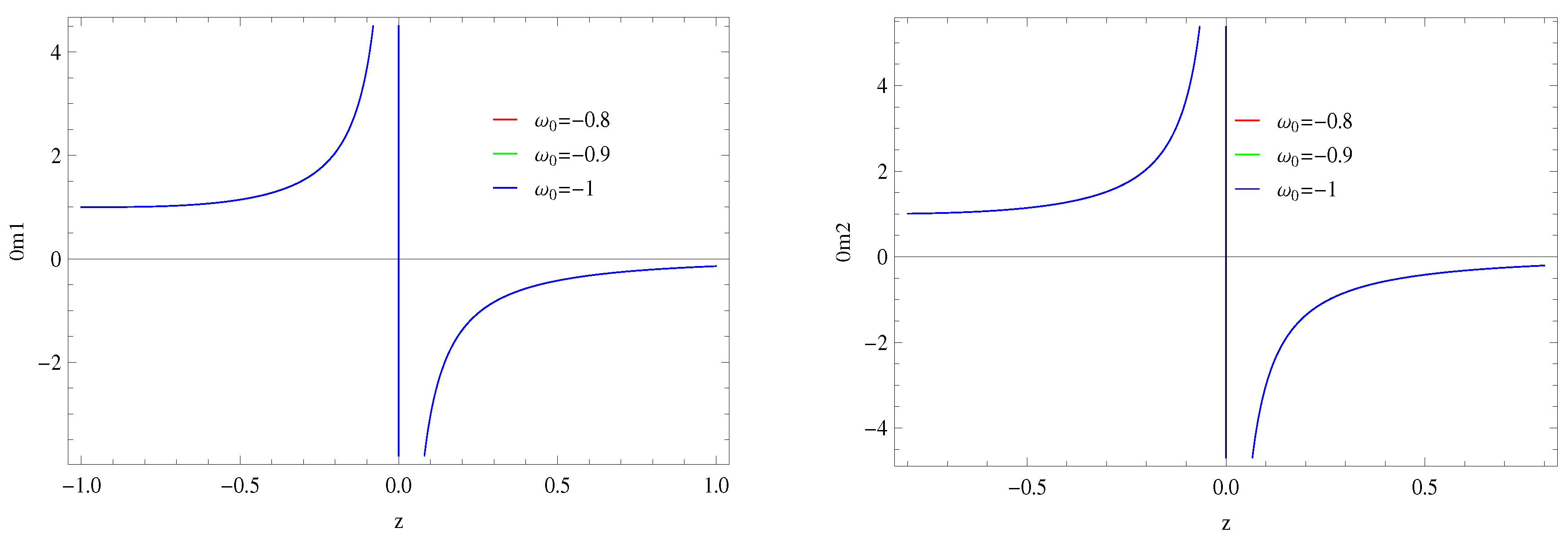
The statefinder parameters ( r , s ) are two new cosmological parameters introduced by Sahni [78] which are defined for flat universe model as
s = r 1 3 ( q 1 2 ) , r = 1 + 3 H ˙ H 2 + H ¨ H 3 ,
which help in differentiating the DE models. That is, for ( r , s ) = ( 1 , 0 ) then it shows the Λ CDM limit, ( r , s ) = ( 1 , 1 ) represents the CDM limit. Also, s > 0 and r < 1 represent the DE regions such that phantom and quintessence and r > 1 , s < 0 give the Chaplygin gas behavior. We can obtain statefinder parameters ( r , s ) for ω 1 d by using Equations (22) and (38) in (45), such that
r 1 = 1 + 3 ( 1 + z ) 2 b 2 ( 1 + z ) 6 2 H 0 2 ( 3 3 c 2 ) ω 0 + A ( 1 + z ) 3 + 3 c 2 ω 0 × ( 9 b 2 ( 1 + z ) 5 H 0 2 ( 3 3 c 2 ω 0 ) + 3 A × ( 1 + z ) 2 + 3 c 2 ω 0 ( 3 + 3 c 2 ω 0 ) ) 1 2 ( b 2 ( 1 + z ) 6 2 H 0 2 ( 3 3 c 2 ) ω 0 + A ( 1 + z ) 3 + 3 c 2 ω 0 ) × 3 b 2 ( 1 + z ) 6 H 0 2 ( 3 3 c 2 ω 0 ) + A ( 1 + z ) 3 + 3 c 2 ω 0 ( 3 + 3 c 2 ω 0 ) ( 15 b 2 ( 1 + z ) 6 H 0 2 ( 3 3 c 2 ω 0 ) + A ( 1 + z ) 3 + 3 c 2 ω 0 ( 3 + 3 c 2 ω 0 ) ( 2 + 3 c 2 ω 0 ) ) ,
s 1 = [ 3 ( 1 + z ) b 2 ( 1 + z ) 6 H 0 2 ( 3 3 c 2 ) ω 0 + 2 A ( 1 + z ) 3 + 3 c 2 ω 0 × ( 9 b 2 ( 1 + z ) 5 H 0 2 ( 3 3 c 2 ω 0 ) + 3 A × ( 1 + z ) 2 + 3 c 2 ω 0 ( 3 + 3 c 2 ω 0 ) ) 1 b 2 ( 1 + z ) 6 H 0 2 ( 3 3 c 2 ) ω 0 + 2 A ( 1 + z ) 3 + 3 c 2 ω 0 × 3 b 2 ( 1 + z ) 6 H 0 2 ( 3 3 c 2 ω 0 ) + A ( 1 + z ) 3 + 3 c 2 ω 0 ( 3 + 3 c 2 ω 0 ) ( 15 b 2 ( 1 + z ) 6 H 0 2 ( 3 3 c 2 ω 0 ) + A ( 1 + z ) 3 + 3 c 2 ω 0 ( 3 + 3 c 2 ω 0 ) ( 2 + 3 c 2 ω 0 ) ) ] [ 3 ( 3 2 ( 1 + z ) × b 2 ( 1 + z ) 6 2 H 0 2 ( 3 3 c 2 ) ω 0 + A ( 1 + z ) 3 + 3 c 2 ω 0 1 × ( 3 b 2 ( 1 + z ) 5 H 0 2 ( 3 3 c 2 ω 0 ) + A ( 1 + z ) 2 + 3 c 2 ω 0 ( 3 + 3 c 2 ω 0 ) ) ) ] 1 .
Inserting Equations (23) and (38) in (45), the statefinder parameters for ω 2 d take the following form
r 2 = 1 + 3 ( 1 + z ) ( b 2 H 0 2 3 3 c 2 ω 0 8 c 2 ω 1 1 3 2 c 2 ω 1 ( 1 + z ) 6 11 c 2 ω 1 1 3 2 c 2 ω 1 + 2 B × ( 1 + z ) 3 + 3 c 2 ω 0 3 c 2 ω 1 1 3 2 c 2 ω 1 ) 1 [ 3 b 2 ( 1 + z ) 6 11 c 2 ω 1 1 3 2 c 2 ω 1 ( 1 3 2 c 2 ω 1 ) ( 6 11 c 2 ω 1 1 3 2 c 2 ω 1 ) 2 H 0 2 ( 3 3 c 2 ω 0 8 c 2 ω 1 ) + 3 B ( 1 + z ) 3 + 3 c 2 ω 0 3 c 2 ω 1 1 3 2 c 2 ω 1 ] [ b 2 H 0 2 ( 3 3 c 2 ω 0 8 c 2 ω 1 1 3 2 c 2 ω 1 ) ( 1 + z ) 6 11 c 2 ω 1 1 3 2 c 2 ω 1 + 2 B ( 1 + z ) 3 + 3 c 2 ω 0 + 3 c 2 ω 1 1 3 2 c 2 ω 1 ] 1 [ ( b 2 ( 1 + z ) 6 11 c 2 ω 1 1 3 2 c 2 ω 1 ( 1 3 2 c 2 ω 1 ) ( 6 11 c 2 ω 1 1 3 2 c 2 ω 1 ) 2 H 0 2 ( 3 3 c 2 ω 0 8 c 2 ω 1 ) + B ( 1 + z ) 3 + 3 c 2 ω 0 3 c 2 ω 1 1 3 2 c 2 ω 1 ) + ( B ( 1 + z ) 3 + 3 c 2 ω 0 3 c 2 ω 1 1 3 2 c 2 ω 1 ( 3 + 3 c 2 ω 0 3 c 2 ω 1 1 3 2 c 2 ω 1 ) ( 2 + 3 c 2 ω 0 3 c 2 ω 1 1 3 2 c 2 ω 1 ) + b 2 ( 1 3 2 c 2 ω 1 ) ( 6 11 c 2 ω 1 1 3 2 c 2 ω 1 ) 2 H 0 2 ( 3 3 c 2 ω 0 8 c 2 ω 1 ) × ( 5 11 c 2 ω 1 1 3 2 c 2 ω 1 ) ( 1 + z ) 6 11 c 2 ω 1 1 3 2 c 2 ω 1 ) ] ,
s 2 = 3 ( 1 + z ) b 2 H 0 2 ( 3 3 c 2 ω 0 8 c 2 ω 1 1 3 2 c 2 ω 1 ) ( 1 + z ) 6 11 c 2 ω 1 1 3 2 c 2 ω 1 + 2 B ( 1 + z ) 3 + 3 c 2 ω 0 3 c 2 ω 1 1 3 2 c 2 ω 1 × [ 3 b 2 ( 1 + z ) 6 11 c 2 ω 1 1 3 2 c 2 ω 1 ( 1 3 2 c 2 ω 1 ) ( 6 11 c 2 ω 1 1 3 2 c 2 ω 1 ) 2 H 0 2 ( 3 3 c 2 ω 0 8 c 2 ω 1 ) + 3 B ( 1 + z ) 3 + 3 c 2 ω 0 × ( 1 + z ) 3 c 2 ω 1 1 3 2 c 2 ω 1 ] [ b 2 H 0 2 ( 3 3 c 2 ω 0 8 c 2 ω 1 1 3 2 c 2 ω 1 ) ( 1 + z ) 6 11 c 2 ω 1 1 3 2 c 2 ω 1 + 2 B × ( 1 + z ) 3 + 3 c 2 ω 0 + 3 c 2 ω 1 1 3 2 c 2 ω 1 ] 1 [ ( b 2 ( 1 + z ) 6 11 c 2 ω 1 1 3 2 c 2 ω 1 ( 1 3 2 c 2 ω 1 ) ( 6 11 c 2 ω 1 1 3 2 c 2 ω 1 ) 2 H 0 2 ( 3 3 c 2 ω 0 8 c 2 ω 1 ) + B ( 1 + z ) 3 + 3 c 2 ω 0 3 c 2 ω 1 1 3 2 c 2 ω 1 ) + ( B ( 1 + z ) 3 + 3 c 2 ω 0 3 c 2 ω 1 1 3 2 c 2 ω 1 ( 3 + 3 c 2 ω 0 3 c 2 ω 1 1 3 2 c 2 ω 1 ) ( 2 + 3 c 2 ω 0 3 c 2 ω 1 1 3 2 c 2 ω 1 ) + b 2 ( 1 3 2 c 2 ω 1 ) ( 6 11 c 2 ω 1 1 3 2 c 2 ω 1 ) 2 H 0 2 ( 3 3 c 2 ω 0 8 c 2 ω 1 ) × ( 5 11 c 2 ω 1 1 3 2 c 2 ω 1 ) ( 1 + z ) 6 11 c 2 ω 1 1 3 2 c 2 ω 1 ) ] [ 3 ( 3 2 ( 1 + z ) × b 2 2 H 0 2 ( 3 3 c 2 ω 0 8 c 2 ω 1 1 3 2 c 2 ω 1 ) ( 1 + z ) 6 11 c 2 ω 1 1 3 2 c 2 ω 1 + B ( 1 + z ) 3 + 3 c 2 ω 0 + 3 c 2 ω 1 1 3 2 c 2 ω 1 1 × 3 B ( 1 + z ) 1 + 3 1 3 2 c 2 ω 1 1 3 2 c 2 ω 1 + b 2 ( 6 11 c 2 ω 1 ) ( 1 + z ) 1 + 6 11 c 2 ω 1 1 3 2 c 2 ω 1 ( 1 3 2 c 2 ω 1 ) H o 2 ( 3 8 c 2 ω 1 1 3 2 c 2 ω 1 3 c 2 ω 0 ) ) ] 1 .
In Figure 5 (left), the graph of s 1 displayed against r 1 for three different values of ω 0 . We can observe that the ( r , s ) parameters corresponds to Chaplygin gas behavior for the underlying scenario. However, the trajectory for ω 0 = 1 does not yield any result for some region which is related to r > 1 , s > 0 . The model constitutes the Λ CDM limit ( r , s ) = ( 1 , 0 ) for the trajectories of ω 0 = 0 . 8 , 0 . 9 . In the right side plot, we draw s 2 versus r 2 for ω 2 d which gives the r < 1 and s > 0 for the trajectory ω 0 = 0 . 9 , ω 1 = 0 . 5 . This shows the DE eras, phantom and quintessence. The remaining two trajectories do not give any fruitful results.

4.4. Om-Diagnostic

The Om-diagnostic is another tool to differentiate different phases of the universe. The positive trajectory of Om-diagnostic represents the DE era like phantom while quintessence era is obtained from negative behavior. This parameter is given by
O m = ( H H 0 ) 2 1 ( 1 + z ) 3 1 .
The Om-diagnostic for ω 1 d and ω 2 d can be obtained by substitution of Equations (22) and (23) in above relation, such that
O m 1 = b 2 ( 1 + z ) 6 2 H 0 2 ( 3 3 c 2 ω 0 ) + A ( 1 + z ) 3 + 3 c 2 ω 0 1 ( 1 + z ) 3 1 ,
O m 2 = b 2 ( 1 + z ) 6 11 c 2 ω 1 1 3 2 c 2 ω 1 2 H 0 2 3 3 c 2 ω 0 8 c 2 ω 1 1 3 2 c 2 ω 1 + B ( 1 + z ) 3 + 3 c 2 ω 0 3 c 2 ω 1 1 3 2 ( c 2 ω 1 ) 1 ( 1 + z ) 3 1 .
In Figure 6, we draw the Om-diagnostic versus z for ω 1 d in left plot and for ω 2 d in the right plot. It can be observed that the trajectories of Om-diagnostic for both cases represent the negative slopes at a past epoch which implies the quintessence era while give positive slopes at future epoch which constitutes the phantom era of the universe.

5. Conclusions

In the framework of dynamical Chern–Simons modified gravity, we have assumed the flat FRW spacetime and discussed different DE models by using a collection of observations at low redshift. We have taken the parametrizations of EoS parameter to explore the cosmic evolution of accelerating universe in interacting scenario. The parametrization may be a Taylor series extension in the redshift, a Taylor series extension in the scale factor or any other parametrization of ω . We have evaluated the different cosmological parameters, such as the deceleration parameter, squared speed of sound, Om-diagnostic and statefinder parameters. The deceleration parameter is a cosmological parameter which helps to classify the accelerated as well as decelerated phases of the universe. The squared speed of sound is another cosmological parameter which is used to check the stability of the models. The statefinder parameters differentiate various DE models, their behavior and cosmological evolution at present time. The Om-diagnostic is used to differentiate the phantom and quintessence behavior. The trajectories of the constructed models have been plotted with different constant parametric values.
The interaction term represented the positive behavior and is observationally verified that the interaction term must not change its sign during cosmic evolution. The deceleration parameter indicated the consistent result while squared speed of sound expressed some stable solutions. The statefinder parameters for the first parametrization represented Chaplygin gas model behavior and met the Λ CDM limit for specific choice of parameters and DE era is obtained for second choice of parametrization. The Om diagnostic parameter indicated the phantom and quintessence eras of the universe.

Author Contributions

A.J., S.R. and S.S. completed the manuscript, while K.B. and R.J. done its proof reading.

Funding

This research received no external funding.

Acknowledgments

S.R. and A.J. are thankful to the Higher Education Commission, Islamabad, Pakistan for its financial support under the grant No: 5412/Federal/NRPU/R&D/HEC/2016. The work of K.B. was partially supported by the JSPS KAKENHI Grant Number JP 25800136 and Competitive Research Funds for Fukushima University Faculty (18RI009).

Conflicts of Interest

The authors declare no conflict of interest.

References

  1. Tripathi, A.; Sangwan, A.; Jassal, H.K. Dark energy equation of state parameter and its evolution at low redshift. JCAP 2017, 06, 012. [Google Scholar] [CrossRef]
  2. Perlmutter, S.; Gabi, S.; Goldhaber, G.; Goobar, A.; Groom, D.E.; Hook, I.M.; Kim, A.G.; Kim, M.Y.; Lee, J.C.; Pain, R.; et al. Measurements* of the Cosmological Parameters Ω and Λ from the First Seven Supernovae at z ≥ 0.35. Astrophys. J. 1997, 483, 565. [Google Scholar] [CrossRef]
  3. Perlmutter, S.; Aldering, G.; Goldhaber, G.; Knop, R.A.; Nugent, P.; Castro, P.G.; Deustua, S.; Fabbro, S.; Goobar, A.; Groom, D.E.; et al. Measurements of Ω and Λ from 42 high-redshift supernovae. Astrophys. J. 1999, 517, 565. [Google Scholar] [CrossRef]
  4. Riess, A.G.; Filippenko, A.V.; Challis, P.; Clocchiatti, A.; Diercks, A.; Garnavich, P.M.; Gillil, R.L.; Hogan, C.J.; Jha, S.; Kirshner, R.P.; et al. Observational evidence from supernovae for an accelerating universe and a cosmological constant. Astron. J. 1998, 116, 1009. [Google Scholar] [CrossRef]
  5. Astier, P.; Guy, J.; Regnault, N.; Pain, R.; Aubourg, E.; Balam, D.; Basa, S.; Carlberg, R.G.; Fabbro, S.; Fouchez, D.; et al. The Supernova Legacy Survey: Measurement of, and w from the first year data set. Astron. Astrophys. J. 2006, 447, 31–48. [Google Scholar] [CrossRef]
  6. Garnavich, P.M.; Jha, S.; Challis, P.; Clocchiatti, A.; Diercks, A.; Filippenko, A.V.; Gillil, R.L.; Hogan, C.J.; Kirshner, R.P.; Leibundgut, B.; et al. Supernova limits on the cosmic equation of state. Astrophys. J. 1998, 509, 74. [Google Scholar] [CrossRef]
  7. Tonry, J.L.; Schmidt, B.P.; Barris, B.; Candia, P.; Challis, P.; Clocchiatti, A.; Coil, A.L.; Filippenko, A.V.; Garnavich, P.; Hogan, C.; et al. Cosmological results from high-z supernovae. Astrophys. J. 2003, 594, 1. [Google Scholar] [CrossRef]
  8. Barris, B.J.; Tonry, J.L.; Blondin, S.; Challis, P.; Chornock, R.; Clocchiatti, A.; Filippenko, A.V.; Garnavich, P.; Holl, S.T.; Jha, S.; et al. Twenty-three high-redshift supernovae from the Institute for Astronomy Deep Survey: Doubling the supernova sample at z > 0.7. Astrophys. J. 2004, 602, 571. [Google Scholar] [CrossRef]
  9. Goobar, A.; Perlmutter, S.; Goldhaber, G.; Knop, R.A.; Nugent, P.; Castro, P.G.; Deustua, S.; Fabbro, S.; Groom, D.E.; Hook, I.M.; et al. The acceleration of the Universe: Measurements of cosmological parameters from type Ia supernovae. Phys. Scr. J. 2000, 85, 47. [Google Scholar] [CrossRef]
  10. González-Gaitán, S.; Conley, A.; Bianco, F.B.; Howell, D.A.; Sullivan, M.; Perrett, K.; Carlberg, R.; Astier, P.; Balam, D.; Ball, C.; et al. The Rise Time of Normal and Subluminous Type Ia Supernovae. Astrophys. J. 2012, 745, 44. [Google Scholar] [CrossRef]
  11. Buckley, J.; Byrum, K.; Dingus, B.; Falcone, A.; Kaaret, P.; Krawzcynski, H.; Pohl, M.; Vassiliev, V.; Williams, D.A. The Status and future of ground-based TeV gamma-ray astronomy. A White Paper prepared for the Division of Astrophysics of the American Physical Society. arXiv 2008, arXiv:0810.0444. [Google Scholar]
  12. Nojiri, S.; Odintsov, S.D. Unified cosmic history in modified gravity: From F(R) theory to Lorentz non-invariant models. Phys. Rep. 2011, 505, 59–144. [Google Scholar] [CrossRef] [Green Version]
  13. Capozziello, S.; Laurentis, M.D. Extended Theories of Gravity. Phys. Rep. 2011, 509, 167–321. [Google Scholar] [CrossRef] [Green Version]
  14. Nojiri, S.; Odintsov, S.D.; Oikonomou, V.K. Modified Gravity Theories on a Nutshell: Inflation, Bounce and Late-time Evolution. Phys. Rep. 2017, 692, 1–104. [Google Scholar] [CrossRef]
  15. Faraoni, V.; Capozziello, S. Beyond Einstein Gravity: A Survey of Gravitational Theories for Cosmology and Astrophysics. Fundam. Theor. Phys. 2010, 170. [Google Scholar] [CrossRef]
  16. Bamba, K.; Odintsov, S.D. Inflationary cosmology in modified gravity theories. Symmetry 2015, 7, 220. [Google Scholar] [CrossRef]
  17. Cai, Y.F.; Capozziello, S.; Laurentis, M.D.; Saridakis, E.N. f(T) teleparallel gravity and cosmology. Rep. Prog. Phys. 2016, 79, 106901. [Google Scholar] [CrossRef]
  18. Pfenniger, D.; Combes, F.; Martinet, L. Is dark matter in spiral galaxies cold gas? I. Observational constraints and dynamical clues about galaxy evolution. Astron. Astrophys. 1994, 285, 79–83. [Google Scholar]
  19. Clowe, D.; Bradač, M.; Gonzalez, A.H.; Markevitch, M.; Rall, S.W.; Jones, C.; Zaritsky, D. A Direct Empirical Proof of the Existence of Dark Matter. Astrophys. J. Lett. 2006, 648, L109–L113. [Google Scholar] [CrossRef]
  20. Alcock, C.; Allsman, R.A.; Axelrod, T.S.; Bennett, D.P.; Cook, K.H.; Freeman, K.C.; Griest, K.; Guern, J.A.; Lehner, M.J.; Marshall, S.L.; et al. The MACHO Project First-Year Large Magellanic Cloud Results: The Microlensing Rate and the Nature of the Galactic Dark Halo. Astrophys. J. 1996, 461, 84. [Google Scholar] [CrossRef]
  21. Zlatev, I.; Wang, L.; Steinhardt, P.J. Quintessence, cosmic coincidence, and the cosmological constant. Phys. Rev. Lett. 1999, 82, 896. [Google Scholar] [CrossRef]
  22. Elizalde, E.; Nojiri, S.; Odinstov, S.D. Late-time cosmology in a (phantom) scalar-tensor theory: Dark energy and the cosmic speed-up. Phys. Rev. D 2004, 70, 043539. [Google Scholar] [CrossRef] [Green Version]
  23. Nojiri, S.; Odintsov, S.D.; Tsujikawa, S. Properties of singularities in the (phantom) dark energy universe. Phys. Rev. D 2005, 71, 063004. [Google Scholar] [CrossRef] [Green Version]
  24. Anisimov, A.; Babichev, E.; Vikman, A. B-Inflation. J. Cosmol. Astropart. Phys. 2005, 6, 006. [Google Scholar] [CrossRef]
  25. Setare, M.R. Interacting generalized Chaplygin gas model in non-flat universe. Eur. Phys. J. C 2007, 52, 689–692. [Google Scholar] [CrossRef] [Green Version]
  26. Bento, M.C.; Bertolami, O.; Sen, A.A. Generalized Chaplygin gas, accelerated expansion, and dark-energy-matter unification. Phys. Rev. D 2002, 66, 043507. [Google Scholar] [CrossRef] [Green Version]
  27. Kamenshchik, A.; Moschella, U.; Pasquier, V. An alternative to quintessence. Phys. Lett. B 2001, 511, 265–268. [Google Scholar] [CrossRef] [Green Version]
  28. Chiba, T.; Okabe, T.; Yamaguchi, M. Kinetically driven quintessence. Phys. Rev. D 2000, 62, 023511. [Google Scholar] [CrossRef] [Green Version]
  29. Armendariz-Picon, C.; Mukhanov, V.; Steinhardt, P. Dynamical Solution to the Problem of a Small Cosmological Constant and Late-Time Cosmic Acceleration. J. Phys. Rev. Lett. 2000, 85, 4438. [Google Scholar] [CrossRef]
  30. Armendariz-Picon, C.; Damour, T.; Mukhanov, V. k-Inflation. Phys. Lett. B 1999, 458, 209–218. [Google Scholar] [CrossRef] [Green Version]
  31. Wei, H.; Cai, R.G. A new model of agegraphic dark energy. Phys. Lett. B 2008, 660, 113–117. [Google Scholar] [CrossRef] [Green Version]
  32. Cai, R.G. A dark energy model characterized by the age of the Universe. Phys. Lett. B 2007, 657, 228–231. [Google Scholar] [CrossRef] [Green Version]
  33. Hsu, S.D.H. Entropy bounds and dark energy. Phys. Lett. B 2004, 594, 13–16. [Google Scholar] [CrossRef] [Green Version]
  34. Li, M. A model of holographic dark energy. Phys. Lett. B 2004, 603, 1–5. [Google Scholar] [CrossRef]
  35. Setare, M.R. The holographic dark energy in non-flat Brans–Dicke cosmology. Phys. Lett. B 2007, 644, 99–103. [Google Scholar] [CrossRef]
  36. Caldwell, R.R. A phantom menace? Cosmological consequences of a dark energy component with super-negative equation of state. Phys. Lett. B 2002, 545, 23–29. [Google Scholar] [CrossRef] [Green Version]
  37. Nojiri, S.; de Odintsov, S.D. Sitter brane universe induced by phantom and quantum effects. Phys. Lett. B 2003, 565, 1–9. [Google Scholar] [CrossRef]
  38. Nojiri, S.; Odintsov, S.D. Quantum de Sitter cosmology and phantom matter. Phys. Lett. B 2003, 562, 147–152. [Google Scholar] [CrossRef] [Green Version]
  39. Tavayef, M.; Sheykhi, A.; Bamba, K.; Moradpour, H. Tsallis holographic dark energy. Phys. Lett. B 2018, 781, 195–200. [Google Scholar] [CrossRef]
  40. Wang, B.; Abdalla, E.; Atrio-Barandela, F.; Pavon, D. Dark matter and dark energy interactions: Theoretical challenges, cosmological implications and observational signatures. Rep. Prog. Phys. 2016, 79, 096901. [Google Scholar] [CrossRef]
  41. Joan, S. Dark energy: A quantum fossil from the inflationary universe? J. Phys. A 2008, 41, 164066. [Google Scholar]
  42. Chevallier, M.; Polarski, D. Accelerating universes with scaling dark matter. Int. J. Mod. Phys. D 2001, 10, 213. [Google Scholar] [CrossRef]
  43. Linder, E.V. Exploring the Expansion History of the Universe. Phys. Rev. Lett. 2003, 90, 091301. [Google Scholar] [CrossRef] [Green Version]
  44. Jassal, H.K.; Bagla, J.S.; Padmanabhan, T. Observational constraints on low redshift evolution of dark energy: How consistent are different observations? Phys. Rev. D 2005, 72, 103503. [Google Scholar] [CrossRef] [Green Version]
  45. Feng, L.; Lu, T. A new equation of state for dark energy model. JCAP 2011, 11, 034. [Google Scholar] [CrossRef]
  46. Efstathiou, G. Constraining the equation of state of the Universe from distant Type Ia supernovae and cosmic microwave background anisotropies. Mon. Not. R. Astron. Soc. 1999, 310, 842. [Google Scholar] [CrossRef]
  47. Lee, S. Constraints on the dark energy equation of state from the separation of CMB peaks and the evolution of α. Phys. Rev. D 2005, 71, 123528. [Google Scholar] [CrossRef]
  48. Hannestad, S.; Mörtsell, E. Cosmological constraints on the dark energy equation of state and its evolution. JCAP 2004, 9, 001. [Google Scholar] [CrossRef]
  49. Wang, Y.; Kostov, V.; Freese, K.; Frieman, J.A.; Gondolo, P. Probing the evolution of the dark energy density with future supernova surveys. JCAP 2004, 12, 003. [Google Scholar] [CrossRef]
  50. Wang, Y.; Tegmark, M. New dark energy constraints from supernovae, microwave background, and galaxy clustering. Phys. Rev. Lett. 2004, 92, 241302. [Google Scholar] [CrossRef]
  51. Bassett, B.A.; Corasaniti, P.S.; Kunz, M. The Essence of Quintessence and the Cost of Compression. Astrophys. J. 2004, 617, L1. [Google Scholar] [CrossRef]
  52. Huterer, D.; Turner, M.S. Prospects for probing the dark energy via supernova distance measurements. Phys. Rev. D 1999, 60, 081301. [Google Scholar] [CrossRef] [Green Version]
  53. Huterer, D.; Turner, M.S. Probing dark energy: Methods and strategies. Phys. Rev. D 2001, 64, 123527. [Google Scholar] [CrossRef] [Green Version]
  54. Weller, J.; Albrecht, A. Opportunities for Future Supernova Studies of Cosmic Acceleration. Phys. Rev. Lett. 2001, 86, 1939. [Google Scholar] [CrossRef]
  55. Pantazis, G.; Nesseris, S.; Perivolaropoulosv, L. Comparison of thawing and freezing dark energy parametrizations. Phys. Rev. D 2016, 93, 103503. [Google Scholar] [CrossRef] [Green Version]
  56. Rani, N.; Jain, D.; Mahajan, S. Transition redshift: new constraints from parametric and nonparametric methods. JCAP 2015, 12, 045. [Google Scholar] [CrossRef]
  57. Copel, E.J.; Sami, M.; Tsujikawa, S. Dynamics of dark energy. Int. J. Mod. Phys. D 2006, 15, 1753. [Google Scholar]
  58. Bamba, K.; Capozziello, S.; Nojiri, S.; Odintsov, S.D. Dark energy cosmology: The equivalent description via different theoretical models and cosmography tests. Astrophys. Space Sci. 2012, 342, 155. [Google Scholar] [CrossRef]
  59. Capozziello, S.; Cardone, V.F.; Elizalde, E.; Nojiri, S.I.; Odintsov, S.D. Observational constraints on dark energy with generalized equations of state. Phys. Rev. D 2006, 73, 043512. [Google Scholar] [CrossRef] [Green Version]
  60. Jackiw, R.; Pi, S.Y. Chern-Simons modification of general relativity. Phys. Rev. D 2003, 68, 104012. [Google Scholar] [CrossRef] [Green Version]
  61. Ashtekar, A.; Balachran, A.P.; Jo, S. The CP problem in quantum gravity. Int. J. Mod. Phys. A 1989, 4, 1493–1514. [Google Scholar] [CrossRef]
  62. Jawad, A.; Sohail, A. Cosmological evolution of modified QCD ghost dark energy in dynamical Chern-Simons gravity. Astrophys. Space Sci. 2015, 55, 359. [Google Scholar] [CrossRef]
  63. Jawad, A.; Rani, S. Cosmological Evolution of Pilgrim Dark Energy in f(G) Gravity. Adv. High Energy Phys. 2015, 10, 952156. [Google Scholar] [CrossRef]
  64. Jawad, A. Reconstruction of f( R ˜ ) models via well-known scale factors. Eur. Phys. J. Plus 2014, 129, 207. [Google Scholar] [CrossRef]
  65. Jawad, A.; Majeed, A. Correspondence of pilgrim dark energy with scalar field models. Astrophy. Space Sci. 2015, 356, 375. [Google Scholar] [CrossRef]
  66. Jawad, A. Cosmological analysis of pilgrim dark energy in loop quantum cosmology. Eur. Phys. J. C 2015, 75, 206. [Google Scholar] [CrossRef]
  67. Jawad, A.; Chattopadhyay, S.; Pasqua, A. A holographic reconstruction of the modifiedf(R) Horava-Lifshitz gravity with scale factor in power-law form. Astrophy. Space Sci. 2013, 346, 273. [Google Scholar] [CrossRef]
  68. Jawad, A.; Chattopadhyay, S.; Pasqua, A. Reconstruction of f(G) gravity with the new agegraphic dark-energy model. Eur. Phys. J. Plus 2013, 128, 88. [Google Scholar] [CrossRef]
  69. Jawad, A.; Pasqua, A.; Chattopadhyay, S. Correspondence between f(G) gravity and holographic dark energy via power-law solution. Astrophy. Space Sci. 2013, 344, 489. [Google Scholar] [CrossRef]
  70. Jawad, A.; Pasqua, A.; Chattopadhyay, S. Holographic reconstruction of f (G) gravity for scale factors pertaining to emergent, logamediate and intermediate scenarios. Eur. Phys. J. Plus 2013, 128, 156. [Google Scholar] [CrossRef]
  71. Jawad, A. Analysis of QCD ghost gravity. Astrophys. Space Sci. 2014, 353, 691. [Google Scholar] [CrossRef]
  72. Younus, M.; Jawad, A.; Qummer, S.; Moradpour, H.; Rani, S. Cosmological Implications of the Generalized Entropy Based Holographic Dark Energy Models in Dynamical Chern-Simons Modified Gravity. Adv. High Energy Phys. 2019, 2019, 1287932. [Google Scholar] [CrossRef]
  73. Cohen, A.; Kaplan, D.; Nelson, A. Effective field theory, black holes, and the cosmological constant. Phys. Rev. Lett. 1999, 82, 4971. [Google Scholar] [CrossRef]
  74. Chattopadhyay, S.; Jawad, A.; Rani, S. Holographic Polytropic Gravity Models. Adv. High Energy Phys. 2015, 2015, 798902. [Google Scholar] [CrossRef]
  75. Jawad, A.; Rani, S.; Salako, I.G.; Gulshan, F. Aspects of some new versions of pilgrim dark energy in DGP braneworld. Eur. Phys. J. Plus 2016, 131, 236. [Google Scholar] [CrossRef]
  76. Elizaldel, E.; Khurshudyan, M.; Nojiri, S. Cosmological singularities in interacting dark energy models with an w(q) parametrization. arxiv 2018, arXiv:1809.01961v1. [Google Scholar]
  77. Cruz, M.; Lepe, S. Holographic approach for dark energy–dark matter interaction in curved FLRW spacetime. Class. Quantum Gravity 2018, 35, 155013. [Google Scholar] [CrossRef]
  78. Sahni, V.; Saini, T.D.; Starobinsky, A.A.; Alam, U. Statefinder—A new geometrical diagnostic of dark energy. JEPT Lett. 2003, 77, 201. [Google Scholar] [CrossRef]
Figure 1. Plot of Q 1 corresponding to z for ω 1 d .
Symmetry 11 01009 g001
Figure 2. Plot of Q 2 corresponding to z for ω 2 d .
Symmetry 11 01009 g002
Figure 3. Plot of q 1 for ω 1 d and q 2 for ω 2 d corresponding to z taking ( ω 0 , ω 1 ) = ( 0 . 8 , 0 . 2 ) , ( 0 . 9 , 0 . 5 ) , ( 1 , 0 . 8 ) .
Symmetry 11 01009 g003
Figure 4. Plot of v s 1 2 for ω 1 d and v s 2 2 for ω 2 d corresponding to z taking ( ω 0 , ω 1 ) = ( 0 . 8 , 0 . 2 ) , ( 0 . 9 , 0 . 5 ) , ( 1 , 0 . 8 ) .
Symmetry 11 01009 g004
Figure 5. Plot of r 1 corresponding to s 1 for ω 1 d and r 2 corresponding to s 2 for ω 2 d .
Symmetry 11 01009 g005
Figure 6. Plot of O m 1 for ω 1 d and O m 2 for ω 2 d corresponding to z.
Symmetry 11 01009 g006

