Numerical Simulation of Pattern Formation on Surfaces Using an Efficient Linear Second-Order Method

Abstract

We present an efficient linear second-order method for a Swift–Hohenberg (SH) type of a partial differential equation having quadratic-cubic nonlinearity on surfaces to simulate pattern formation on surfaces numerically. The equation is symmetric under a change of sign of the density field if there is no quadratic nonlinearity. We introduce a narrow band neighborhood of a surface and extend the equation on the surface to the narrow band domain. By applying a pseudo-Neumann boundary condition through the closest point, the Laplace–Beltrami operator can be replaced by the standard Laplacian operator. The equation on the narrow band domain is split into one linear and two nonlinear subequations, where the nonlinear subequations are independent of spatial derivatives and thus are ordinary differential equations and have closed-form solutions. Therefore, we only solve the linear subequation on the narrow band domain using the Crank–Nicolson method. Numerical experiments on various surfaces are given verifying the accuracy and efficiency of the proposed method.

1. Introduction

A Swift–Hohenberg (SH) type of partial differential equation [1] has been used to study pattern formation [2,3,4,5]:

$$\begin{array}{c}\hfill \frac{\partial \varphi }{\partial t}=-\left({\varphi }^3-g{\varphi }^2+\left(-ϵ+{(1+\Delta )}^2\right)\varphi \right),\end{array}$$

where $\varphi$ is the density field and $g\ge 0$ and $ϵ>0$ are constants. In general, the equation does not have an analytical solution, thus various computational algorithms [6,7,8,9,10,11,12,13] have been proposed to obtain a numerical solution. However, most of them were solved on flat surfaces except [12,13].

In this paper, we present an efficient linear second-order method for the SH type of equation on surfaces, which is based on the closest point method [14,15]. We introduce a narrow band domain of a surface and apply a pseudo-Neumann boundary condition on the boundary of the narrow band domain through the closest point [16]. This results in a constant value of $\varphi$ in the direction normal to the surface, thus the Laplace–Beltrami operator can be replaced by the standard Laplacian operator. In addition, we split the equation into one linear and two nonlinear subequations [17,18], where the nonlinear subequations are independent of spatial derivatives and thus are ordinary differential equations and have closed-form solutions. Therefore, we only solve the linear subequation on the narrow band domain using the Crank–Nicolson method. As a result, our method is easy to implement and linear.

This paper is organized as follows. In Section 2, we describe the SH type of equation on a narrow band domain. In Section 3, we propose an efficient linear second-order method for the equation on the narrow band domain. Numerical examples on various surfaces are given in Section 4. Finally, we conclude in Section 5.

2. Swift–Hohenberg Type of Equation on a Narrow Band Domain

The SH type of equation on a surface $\mathcal{S}$ is given by

$$\begin{array}{c}\hfill \frac{\partial \varphi (\mathbf{x},t)}{\partial t}=-\left({\varphi }^3(\mathbf{x},t)-g{\varphi }^2(\mathbf{x},t)+\left(-ϵ+{(1+{\Delta }_{\mathcal{S}})}^2\right)\varphi (\mathbf{x},t)\right),\mathbf{x}\in \mathcal{S},0<t\le T,\end{array}$$

(1)

where ${\Delta }_{\mathcal{S}}$ is the Laplace–Beltrami operator [19,20]. Next, let ${\mathrm{\Omega }}_{\delta }=\left\{\mathbf{y}\right|\mathbf{x}\in \mathcal{S},\mathbf{y}=\mathbf{x}+\eta \mathbf{n}\left(\mathbf{x}\right)\mathrm{for}\left|\eta \right|<\delta \}$ be a $\delta$-neighborhood of $\mathcal{S}$, where $\mathbf{n}\left(\mathbf{x}\right)$ is a unit normal vector at $\mathbf{x}$. Then, we extend the Equation (1) to the narrow band domain ${\mathrm{\Omega }}_{\delta }$:

$$\begin{array}{c}\hfill \frac{\partial \varphi (\mathbf{x},t)}{\partial t}=-\left({\varphi }^3(\mathbf{x},t)-g{\varphi }^2(\mathbf{x},t)+\left(-ϵ+{(1+{\Delta }_{\mathcal{S}})}^2\right)\varphi (\mathbf{x},t)\right),\mathbf{x}\in {\mathrm{\Omega }}_{\delta },0<t\le T\end{array}$$

(2)

with the pseudo-Neumann boundary condition on $\partial {\mathrm{\Omega }}_{\delta }$:

$$\begin{array}{c}\hfill \varphi (\mathbf{x},t)=\varphi \left(\mathrm{cp}\right(\mathbf{x}),t),\end{array}$$

(3)

where $\mathrm{cp}\left(\mathbf{x}\right)$ is a point on $\mathcal{S}$, which is closest to $\mathbf{x}\in \partial {\mathrm{\Omega }}_{\delta }$ [14]. For a sufficiently small $\delta$, $\varphi$ is constant in the direction normal to the surface. Thus, the Laplace–Beltrami operator in ${\mathrm{\Omega }}_{\delta }$ can be replaced by the standard Laplacian operator [14], i.e.,

$$\begin{array}{c}\hfill \frac{\partial \varphi (\mathbf{x},t)}{\partial t}=-\left({\varphi }^3(\mathbf{x},t)-g{\varphi }^2(\mathbf{x},t)+\left(-ϵ+{(1+\Delta )}^2\right)\varphi (\mathbf{x},t)\right),\mathbf{x}\in {\mathrm{\Omega }}_{\delta },0<t\le T.\end{array}$$

(4)

3. Numerical Method

In this section, we propose an efficient linear second-order method for solving Equation (4) with the boundary condition (3). We discretize Equation (4) in $\mathrm{\Omega }=[-L_x/2,L_x/2]\times [-L_y/2,L_y/2]\times [-L_z/2,L_z/2]$ that includes ${\mathrm{\Omega }}_{\delta }$. Let $h=L_x/N_x=L_y/N_y=L_z/N_z$ be the uniform grid size, where $N_x$, $N_y$, and $N_z$ are positive integers. Let ${\mathrm{\Omega }}^h=\{{\mathbf{x}}_{ijk}=(x_i,y_j,z_k)|x_i=-L_x/2+ih,y_j=-L_y/2+jh,z_k=-L_z/2+kh\mathrm{for}0\le i\le N_x,0\le j\le N_y,0\le k\le N_z\}$ be a discrete domain. Let ${\varphi }_{ijk}^n$ be an approximation of $\varphi ({\mathbf{x}}_{ijk},n\Delta t)$, where $\Delta t$ is the time step. Let ${\mathrm{\Omega }}_{\delta }^h=\{{\mathbf{x}}_{ijk}\left|\right|{\psi }_{ijk}|<\delta \}$ be a discrete narrow band domain, where $\psi$ is a signed distance function for the surface $\mathcal{S}$, and $\partial {\mathrm{\Omega }}_{\delta }^h=\{{\mathbf{x}}_{ijk}|I_{ijk}|{\nabla }_h{I}_{ijk}|\ne 0\}$ are discrete domain boundary points, where ${\nabla }_h{I}_{ijk}=(I_{i+1,j,k}-I_{i-1,j,k},I_{i,j+1,k}-I_{i,j-1,k},I_{i,j,k+1}-I_{i,j,k-1})/\left(2h\right)$. Here, $I_{ijk}=0$ if ${\mathbf{x}}_{ijk}\in {\mathrm{\Omega }}_{\delta }^h$, and $I_{ijk}=1$, otherwise.

We here split Equation (4) into the following subequations:

$$\begin{array}{ccc}\hfill \frac{\partial \varphi }{\partial t}& =& -({\varphi }^3-ϵ\varphi ),\hfill \end{array}$$

(5)

$$\begin{array}{ccc}\hfill \frac{\partial \varphi }{\partial t}& =& g{\varphi }^2,\hfill \end{array}$$

(6)

$$\begin{array}{ccc}\hfill \frac{\partial \varphi }{\partial t}& =& -{(1+\Delta )}^2\varphi .\hfill \end{array}$$

(7)

Equations (5) and (6) are solved analytically and the solutions ${\varphi }_{ijk}^{n+1}$ are given as follows:

$$\begin{array}{c}\hfill {\varphi }_{ijk}^{n+1}=\frac{{\varphi }_{ijk}^n}{\sqrt{{\left({\varphi }_{ijk}^n\right)}^2/ϵ+(1-{\left({\varphi }_{ijk}^n\right)}^2/ϵ)e^{-2ϵ\Delta t}}}\mathrm{and}{\varphi }_{ijk}^{n+1}=\frac{{\varphi }_{ijk}^n}{1-g\Delta t{\varphi }_{ijk}^n},\end{array}$$

respectively. In addition, Equation (7) is solved using the Crank–Nicolson method:

$$\begin{array}{c}\hfill \frac{{\varphi }_{ijk}^{n+1}-{\varphi }_{ijk}^n}{\Delta t}=-\frac{{(1+{\Delta }_h)}^2}{2}({\varphi }_{ijk}^{n+1}+{\varphi }_{ijk}^n)\end{array}$$

(8)

with the boundary condition on $\partial {\mathrm{\Omega }}_{\delta }^h$:

$$\begin{array}{c}\hfill {\varphi }_{ijk}^n={\varphi }^n\left(\mathrm{cp}\left({\mathbf{x}}_{ijk}\right)\right).\end{array}$$

Here, ${\Delta }_h{\varphi }_{ijk}=({\varphi }_{i+1,j,k}+{\varphi }_{i-1,j,k}+{\varphi }_{i,j+1,k}+{\varphi }_{i,j-1,k}+{\varphi }_{i,j,k+1}+{\varphi }_{i,j,k-1}-6{\varphi }_{ijk})/h^2$. The numerical closest point $\mathrm{cp}\left({\mathbf{x}}_{ijk}\right)$ for a point ${\mathbf{x}}_{ijk}\in \partial {\mathrm{\Omega }}_{\delta }^h$ is defined as

$$\begin{array}{c}\hfill \mathrm{cp}\left({\mathbf{x}}_{ijk}\right)={\mathbf{x}}_{ijk}-\left|{\psi }_{ijk}\right|\frac{{\nabla }_h\left|{\psi }_{ijk}\right|}{|{\nabla }_h|{\psi }_{ijk}\left|\right|}.\end{array}$$

In general, $\mathrm{cp}\left({\mathbf{x}}_{ijk}\right)$ is not a grid point in ${\mathrm{\Omega }}_{\delta }^h$, i.e., $\mathrm{cp}\left({\mathbf{x}}_{ijk}\right)\notin {\mathrm{\Omega }}_{\delta }^h$, and thus we use trilinear interpolation and take $\delta >\sqrt{3}h$ to obtain $\varphi \left(\mathrm{cp}\left({\mathbf{x}}_{ijk}\right)\right)$. The resulting implicit linear discrete system of Equation (8) is solved efficiently using the Jacobi iterative method. We iterate the Jacobi iteration until a discrete $L^2$-norm of the consecutive error on ${\mathrm{\Omega }}_{\delta }^h$ is less than a tolerance $tol$. Here, the discrete $L^2$-norm on ${\mathrm{\Omega }}_{\delta }^h$ is defined as ${\parallel \varphi \parallel }_{L^2\left({\mathrm{\Omega }}_{\delta }^h\right)}=\sqrt{{\sum }_{{\mathbf{x}}_{ijk}\in {\mathrm{\Omega }}_{\delta }^h}{\varphi }_{ijk}^2/\#{\mathrm{\Omega }}_{\delta }^h}$, where $\#{\mathrm{\Omega }}_{\delta }^h$ is the cardinality of ${\mathrm{\Omega }}_{\delta }^h$. Then, the second-order solution of Equation (4) is evolved by five stages [21]

$$\begin{array}{ccc}\hfill {\varphi }_{ijk}^{\left(1\right)}& =& \frac{{\varphi }_{ijk}^n}{\sqrt{{\left({\varphi }_{ijk}^n\right)}^2/ϵ+(1-{\left({\varphi }_{ijk}^n\right)}^2/ϵ)e^{-ϵ\Delta t}}},\hfill \\ \hfill {\varphi }_{ijk}^{\left(2\right)}& =& \frac{{\varphi }_{ijk}^{\left(1\right)}}{1-(g\Delta t/2){\varphi }_{ijk}^{\left(1\right)}},\hfill \\ \hfill \frac{{\varphi }_{ijk}^{\left(3\right)}-{\varphi }_{ijk}^{\left(2\right)}}{\Delta t}& =& -\frac{{(1+{\Delta }_h)}^2}{2}({\varphi }_{ijk}^{\left(3\right)}+{\varphi }_{ijk}^{\left(2\right)}),\hfill \\ \hfill {\varphi }_{ijk}^{\left(4\right)}& =& \frac{{\varphi }_{ijk}^{\left(3\right)}}{1-(g\Delta t/2){\varphi }_{ijk}^{\left(3\right)}},\hfill \\ \hfill {\varphi }_{ijk}^{n+1}& =& \frac{{\varphi }_{ijk}^{\left(4\right)}}{\sqrt{{\left({\varphi }_{ijk}^{\left(4\right)}\right)}^2/ϵ+(1-{\left({\varphi }_{ijk}^{\left(4\right)}\right)}^2/ϵ)e^{-ϵ\Delta t}}}.\hfill \end{array}$$

4. Numerical Experiments

4.1. Convergence Test

In order to verify the rate of convergence of the proposed method, we consider the evolution of $\varphi$ on a unit sphere. An initial piece of data is

$$\begin{array}{c}\hfill \varphi (x,y,z,0)=0.15+0.1\cos \left(2\pi x\right)\cos \left(2\pi y\right)\cos \left(2\pi z\right)\end{array}$$

and a signed distance function for the unit sphere is

$$\begin{array}{c}\hfill \psi (x,y,z)=\sqrt{x^2+y^2+z^2}-1\end{array}$$

on $\mathrm{\Omega }={[-1.5,1.5]}^3$. We fix the grid size to $h=0.125$ and vary $\Delta t=T/2,T/2^2,T/2^3,T/2^4$ for $T=0.00025$ with $ϵ=0.25$, $\delta =2.2\sqrt{3}h$, and $tol=\Delta t$. Table 1 shows the $L^2$-errors of $\varphi (x,y,z,T)$ and convergence rates with $g=0$. Here, the errors are computed by comparison with a reference numerical solution using $\Delta t=T/2^6$. It is observed that the method is second-order accurate in time. Note that we obtain the same result for $g=1$.

Table 1. $L^2$-errors and convergence rates for $g=0$.

$\mathsf{\Delta }\mathit{t}$	$\mathit{T}/2$		$\mathit{T}/2^2$		$\mathit{T}/2^3$		$\mathit{T}/2^4$
$L^2$-error	$5.445\times {10}^{-3}$		$1.341\times {10}^{-3}$		$2.862\times {10}^{-4}$		$5.519\times {10}^{-5}$
Rate		2.02		2.22		2.37

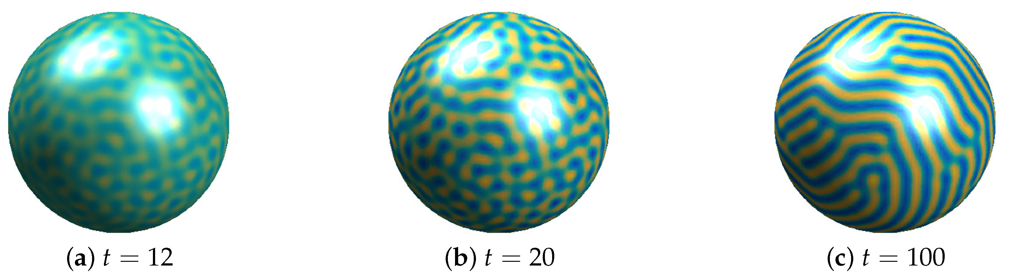
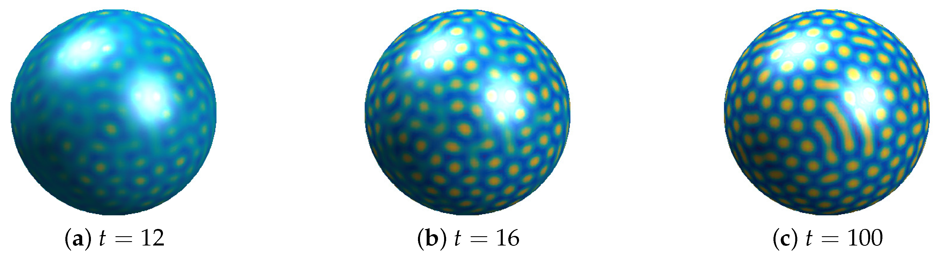
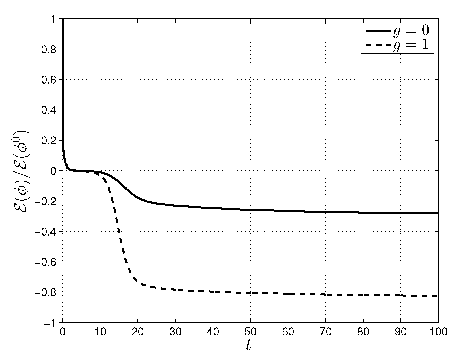
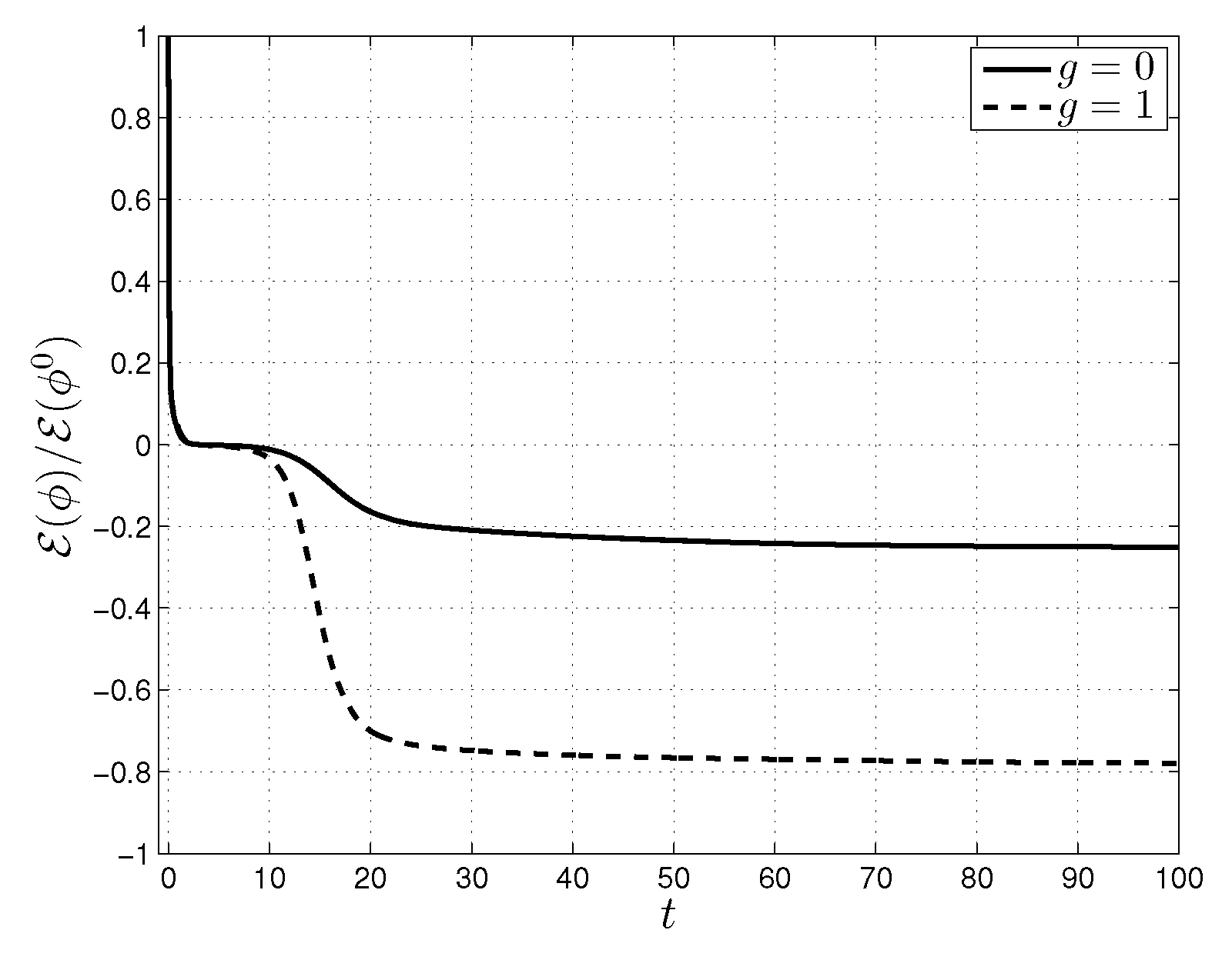
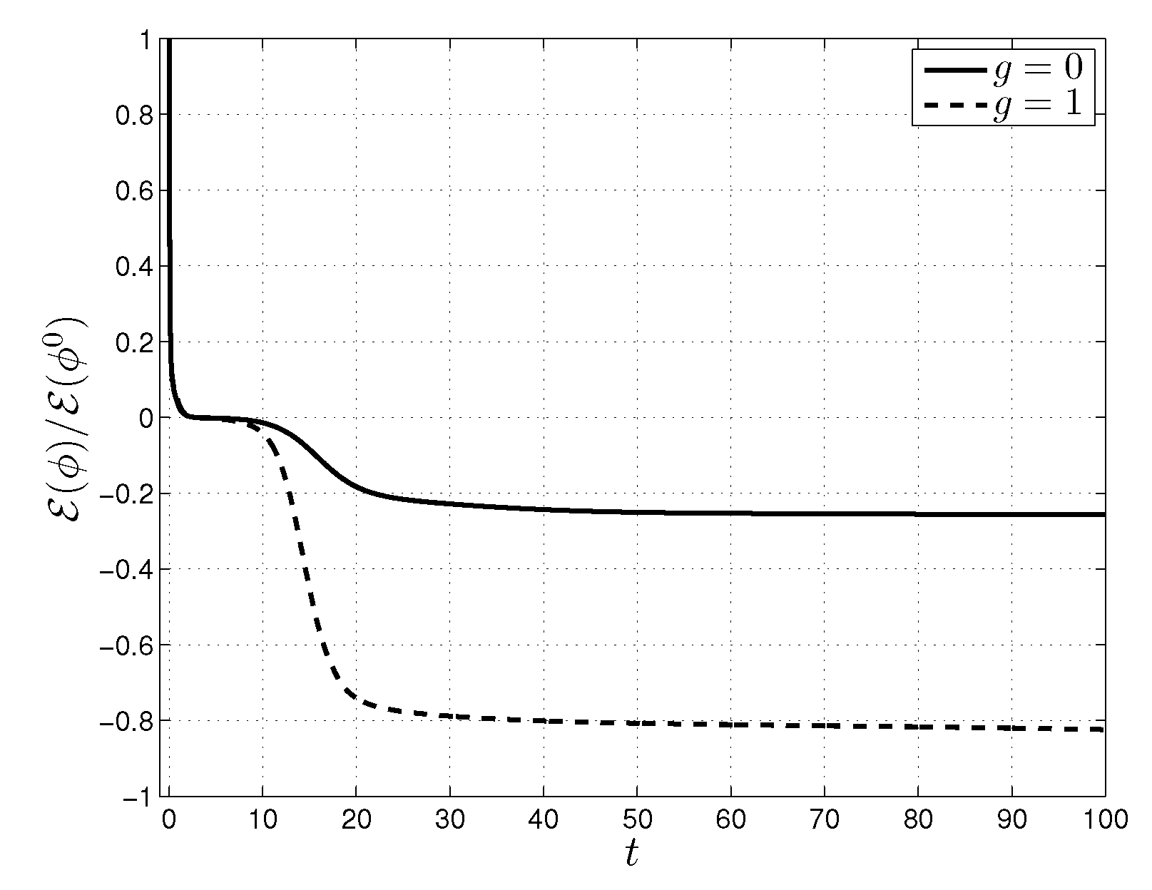
4.2. Pattern Formation on a Sphere

Unless otherwise stated, we take an initial piece of data as

$$\begin{array}{c}\hfill \varphi (x,y,z,0)=0.15+\mathrm{rand}(x,y,z),\end{array}$$

where $\mathrm{rand}(x,y,z)$ is a uniformly distributed random number between $-0.1$ and $0.1$ at the grid points, and use $ϵ=0.25$, $h=1$, $\Delta t=0.1$, $\delta =1.1\sqrt{3}h$, and $tol={10}^{-4}$.

For $g=0$ and 1, Figure 1 and Figure 2 show the evolution of $\varphi (x,y,z,t)$ on a sphere with $\psi (x,y,z)=\sqrt{x^2+y^2+z^2}-32$ on $\mathrm{\Omega }={[-36,36]}^3$, respectively. Depending on the value of g, we have different patterns, such as striped (Figure 1) and hexagonal (Figure 2) [11]. Figure 3 shows the energy decay with $g=0$ and 1, where the energy $\mathcal{E}\left(\varphi \right)$ is defined by

$$\begin{array}{c}\hfill \mathcal{E}\left(\varphi \right)={\int }_{{\mathrm{\Omega }}_{\delta }}\left(\frac{1}{4}{\varphi }^4-\frac{g}{3}{\varphi }^3+\frac{1}{2}\varphi \left(-ϵ+{(1+\Delta )}^2\right)\varphi \right)d\mathbf{x}.\end{array}$$

Figure 1. Evolution of $\varphi (x,y,z,t)$ with $g=0$. The yellow and blue regions indicate $\varphi =0.7540$ and $-0.7783$, respectively.

Figure 2. Evolution of $\varphi (x,y,z,t)$ with $g=1$. The yellow and blue regions indicate $\varphi =1.4320$ and $-0.7152$, respectively.

Figure 3. Evolution of $\mathcal{E}\left(\varphi \right)/\mathcal{E}\left({\varphi }^0\right)$ on the sphere with $g=0$ and 1.

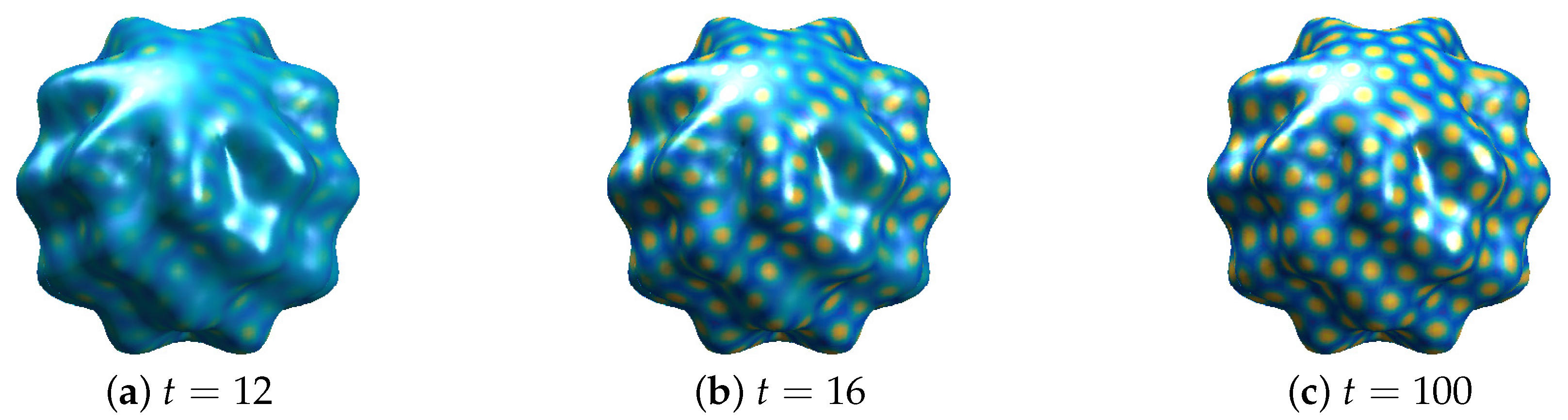
4.3. Pattern Formation on a Sphere Perturbed by a Spherical Harmonic

In this section, we perform the evolution of $\varphi$ on a sphere of center $(0,0,0)$ and radius 32 perturbed by a spherical harmonic $10Y_{10}^7(\theta ,\phi )$. Here, $\theta$ and $\phi$ are the polar and azimuthal angles, respectively, and the computational domain is $\mathrm{\Omega }={[-40,40]}^3$. Figure 4 and Figure 5 show the evolution of $\varphi (x,y,z,t)$ with $g=0$ and 1, respectively. From the results in Figure 4 and Figure 5, we can see that our method can solve the SH type of equation on not only simple but also complex surfaces. Figure 6 shows the energy decay with $g=0$ and 1.

Figure 4. Evolution of $\varphi (x,y,z,t)$ with $g=0$. The yellow and blue regions indicate $\varphi =0.8717$ and $-0.8372$, respectively.

Figure 5. Evolution of $\varphi (x,y,z,t)$ with $g=1$. The yellow and blue regions indicate $\varphi =1.4833$ and $-0.7135$, respectively.

Figure 6. Evolution of $\mathcal{E}\left(\varphi \right)/\mathcal{E}\left({\varphi }^0\right)$ on the perturbed sphere with $g=0$ and 1.

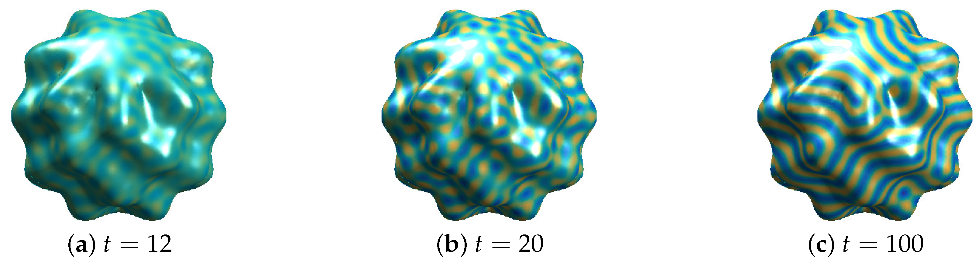
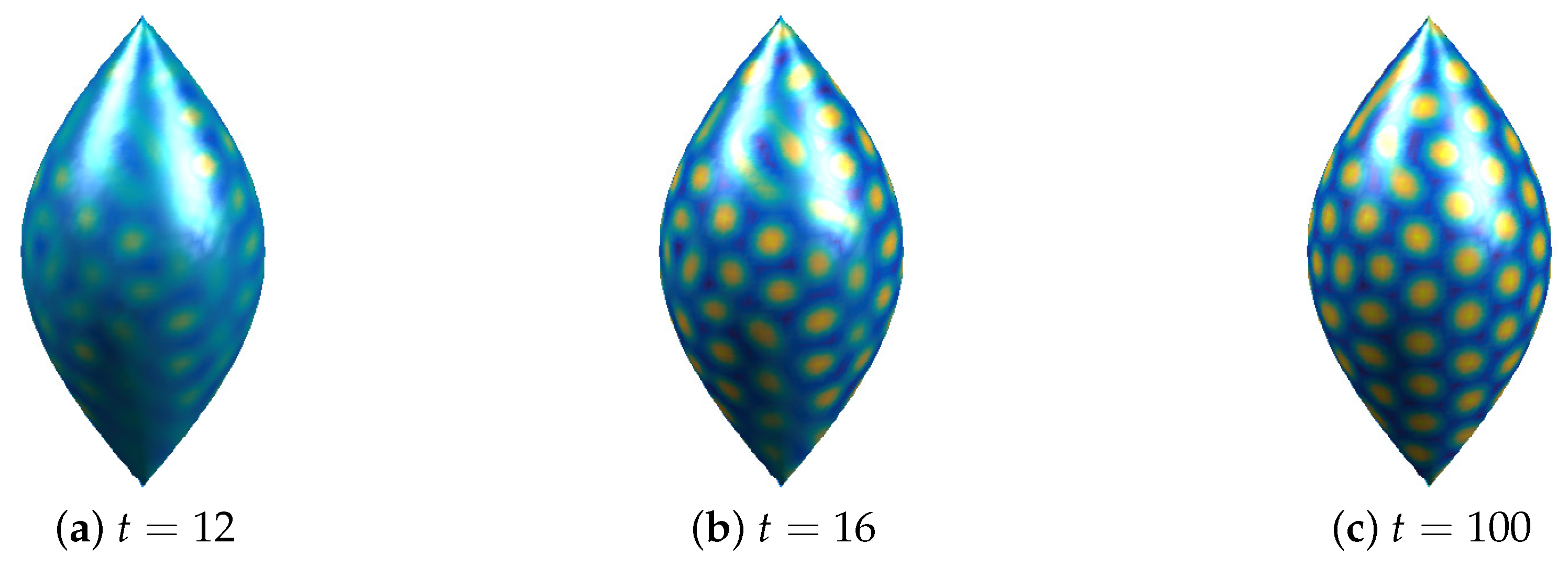
4.4. Pattern Formation on a Spindle

Finally, we simulate the evolution of $\varphi$ on a spindle that has narrow and sharp tips. The spindle is defined parametrically as

$$\begin{array}{c}\hfill x=16\cos \theta \sin \phi ,y=16\sin \theta \sin \phi ,z=32\left(\frac{2\phi }{\pi }-1\right),\end{array}$$

where $\theta \in [0,2\pi )$ and $\phi \in [0,\pi )$, and the computational domain is $\mathrm{\Omega }=[-20,20]\times [-20,20]\times [-36,36]$. Figure 7 and Figure 8 show the evolution of $\varphi (x,y,z,t)$ with $g=0$ and 1, respectively. The results in Figure 7 and Figure 8 suggest that pattern formation on a surface having narrow and sharp tips can be simulated by using our method. Figure 9 shows the energy decay with $g=0$ and 1.

Figure 7. Evolution of $\varphi (x,y,z,t)$ with $g=0$. The yellow and blue regions indicate $\varphi =0.7059$ and $-0.7593$, respectively.

Figure 8. Evolution of $\varphi (x,y,z,t)$ with $g=1$. The yellow and blue regions indicate $\varphi =1.3842$ and $-0.6224$, respectively.

Figure 9. Evolution of $\mathcal{E}\left(\varphi \right)/\mathcal{E}\left({\varphi }^0\right)$ on the spindle with $g=0$ and 1.

5. Conclusions

We simulated pattern formation on surfaces numerically by solving the SH type of equation on surfaces by using the efficient linear second-order method. The method was based on the closest point and operator splitting methods and thus was easy to implement and linear. We confirmed that the proposed method gives the desired order of accuracy in time and observed that pattern formation on surfaces is affected by the value of g.

References

- Swift, J.; Hohenberg, P.C. Hydrodynamic fluctuations at the convective instability. Phys. Rev. A 1977, 15, 319–328. [Google Scholar] [CrossRef]
- Hohenberg, P.C.; Swift, J.B. Effects of additive noise at the onset of Rayleigh–Bénard convection. Phys. Rev. A 1992, 46, 4773–4785. [Google Scholar] [CrossRef] [PubMed]
- Cross, M.C.; Hohenberg, P.C. Pattern formation outside of equilibrium. Rev. Mod. Phys. 1993, 65, 851–1112. [Google Scholar] [CrossRef]
- Rosa, R.R.; Pontes, J.; Christov, C.I.; Ramos, F.M.; Rodrigues Neto, C.; Rempel, E.L.; Walgraef, D. Gradient pattern analysis of Swift–Hohenberg dynamics: Phase disorder characterization. Phys. A 2000, 283, 156–159. [Google Scholar] [CrossRef]
- Hutt, A.; Atay, F.M. Analysis of nonlocal neural fields for both general and gamma-distributed connectivities. Phys. D 2005, 203, 30–54. [Google Scholar] [CrossRef]
- Cheng, M.; Warren, J.A. An efficient algorithm for solving the phase field crystal model. J. Comput. Phys. 2008, 227, 6241–6248. [Google Scholar] [CrossRef]
- Wise, S.M.; Wang, C.; Lowengrub, J.S. An energy-stable and convergent finite-difference scheme for the phase field crystal equation. SIAM J. Numer. Anal. 2009, 47, 2269–2288. [Google Scholar] [CrossRef]
- Gomez, H.; Nogueira, X. A new space–time discretization for the Swift–Hohenberg equation that strictly respects the Lyapunov functional. Commun. Nonlinear Sci. Numer. Simul. 2012, 17, 4930–4946. [Google Scholar] [CrossRef]
- Elsey, M.; Wirth, B. A simple and efficient scheme for phase field crystal simulation. ESAIM: Math. Model. Numer. Anal. 2013, 47, 1413–1432. [Google Scholar] [CrossRef]
- Sarmiento, A.F.; Espath, L.F.R.; Vignal, P.; Dalcin, L.; Parsani, M.; Calo, V.M. An energy-stable generalized-α method for the Swift–Hohenberg equation. J. Comput. Appl. Math. 2018, 344, 836–851. [Google Scholar] [CrossRef]
- Lee, H.G. An energy stable method for the Swift–Hohenberg equation with quadratic–cubic nonlinearity. Comput. Methods Appl. Mech. Eng. 2019, 343, 40–51. [Google Scholar] [CrossRef]
- Matthews, P.C. Pattern formation on a sphere. Phys. Rev. E 2003, 67, 036206. [Google Scholar] [CrossRef] [PubMed]
- Sigrist, R.; Matthews, P. Symmetric spiral patterns on spheres. SIAM J. Appl. Dyn. Syst. 2011, 10, 1177–1211. [Google Scholar] [CrossRef][Green Version]
- Ruuth, S.J.; Merriman, B. A simple embedding method for solving partial differential equations on surfaces. J. Comput. Phys. 2008, 227, 1943–1961. [Google Scholar] [CrossRef]
- Choi, Y.; Jeong, D.; Lee, S.; Yoo, M.; Kim, J. Motion by mean curvature of curves on surfaces using the Allen–Cahn equation. Int. J. Eng. Sci. 2015, 97, 126–132. [Google Scholar] [CrossRef]
- Lee, H.G.; Kim, J. A simple and efficient finite difference method for the phase-field crystal equation on curved surfaces. Comput. Methods Appl. Mech. Eng. 2016, 307, 32–43. [Google Scholar] [CrossRef]
- Pak, D.; Han, C.; Hong, W.-T. Iterative speedup by utilizing symmetric data in pricing options with two risky assets. Symmetry 2017, 9, 12. [Google Scholar] [CrossRef]
- Zong, C.; Tang, Y.; Cho, Y.J. Convergence analysis of an inexact three-operator splitting algorithm. Symmetry 2018, 10, 563. [Google Scholar] [CrossRef]
- Bertalmío, M.; Cheng, L.-T.; Osher, S.; Sapiro, G. Variational problems and partial differential equations on implicit surfaces. J. Comput. Phys. 2001, 174, 759–780. [Google Scholar] [CrossRef]
- Greer, J.B. An improvement of a recent Eulerian method for solving PDEs on general geometries. J. Sci. Comput. 2006, 29, 321–352. [Google Scholar] [CrossRef]
- Strang, G. On the construction and comparison of difference schemes. SIAM J. Numer. Anal. 1968, 5, 506–517. [Google Scholar] [CrossRef]
© 2019 by the author. Licensee MDPI, Basel, Switzerland. This article is an open access article distributed under the terms and conditions of the Creative Commons Attribution (CC BY) license (http://creativecommons.org/licenses/by/4.0/).