A Deviation-Based Dynamic Vertex Reordering Technique for 2D Mesh Quality Improvement

Abstract

We propose a novel deviation-based vertex reordering method for 2D mesh quality improvement. We reorder free vertices based on how likely this is to improve the quality of adjacent elements, based on the gradient of the element quality with respect to the vertex location. Specifically, we prioritize the free vertex with large differences between the best and the worst-quality element around the free vertex. Our method performs better than existing vertex reordering methods since it is based on the theory of non-smooth optimization. The downhill simplex method is employed to solve the mesh optimization problem for improving the worst element quality. Numerical results show that the proposed vertex reordering techniques improve both the worst and average element, compared to those with existing vertex reordering techniques.

1. Introduction

When the finite element method (FEM) is used to solve certain partial differential equations (PDEs), the quality of a mesh element is determined geometrically. For instance, to solve the Poisson equation, equilateral elements are preferred over “long and skinny” ones [1,2]. In order to measure the quality of a triangle, the ratio of the radius of the incircle and the circumcircle may be used. The ratio is maximal for an equilateral triangle and tends to zero as the triangle becomes degenerate [1], so it serves as a good measure of the quality of a triangle. The quality of the whole mesh is typically defined as some average (mean, r.m.s., etc.) of the quality of its elements [1,3].

The FEM is faster and more accurate if the mesh is of high quality [1]. In order to obtain a high-quality mesh, numerical optimization algorithms may be used to move mesh vertices such that the quality of the elements improves. Since the quality of the elements is a continuous function of the position of the vertices, several papers have explored the use of different continuous numerical optimization techniques to efficiently carry out the quality improvement [4,5,6].

The objective function that is optimized by the numerical techniques can be formulated in the following two ways: (a) global formulation and (b) local formulation. In the global formulation, every vertex in the mesh contributes to the objective function (an average mesh quality) that is being optimized. In other words, in every iteration, all vertices are simultaneously moved to improve the mesh quality. In the local formulation, only one vertex contributes to the objective function being optimized in each step. In other words, in each step, only one vertex is moved, and other vertices wait for their turn to move.

In the local mesh optimization technique, a natural question arises about the order in which the vertices are moved: is it possible to further improve the mesh quality or the efficiency (fewer iterations/less time) of the optimization by changing the vertex ordering? The ordering of vertices is especially important when the mesh quality is defined as the quality of its worst-quality element. Can we prioritize vertices that belong to the worst-quality element? In this paper, we answer this question by analyzing the objective function that we are attempting to optimize. In particular, we consider the problem of improving the quality of the worst-quality element in a mesh because it significantly affects the efficiency and accuracy of the FEM.

Sastry et al. developed a global formulation for the objective function based on the log-barrier technique, which improved the quality of all poor elements in a mesh, not just the worst one [7]. A global formulation is sometimes too expensive since all we really need is a way to improve the quality of few poor elements in a mesh. Thus, local techniques may be preferred for this purpose because it takes much less time.

We attempted to improve the quality of the worst element using the active set method, [8,9] which is a local technique. We found that quality of the worst element improves only in the first few iterations, but the quality remains static in the subsequent iterations. This was because the worst-quality element was surrounded by other poor-quality elements. By moving any of the vertices of the worst-quality element, the adjacent poor-quality elements would become poorer. Thus, the optimization routine was stuck in a local optimum in the part of the mesh where the worst-quality element was present. In other parts of the mesh, however, we saw some significant vertex movement. In those parts, we observed that there were both high- and poor-quality elements, and the quality of the poor elements were being improved at the cost of the quality of good elements. This observation led us to develop our inequality-based vertex reordering technique.

A high inequality in the quality of elements around a vertex is indicative (though not necessarily) of a high potential of quality improvement around the vertex. When the vertex moves appropriately, the quality of poor elements improves, and the quality of good elements deteriorates. Thus, we end up with elements of nearly identical quality around the vertex. After the vertex movement, the quality of the neighbors of the (formerly) good elements remains unchanged because we move only one vertex at a time. As a result, we have propagated the inequality with respect to the mesh quality from one vertex to the neighboring vertex. When the propagation hits a vertex with the worst-quality element, it is possible to improve the quality of the worst element in subsequent iterations. The propagation of the inequality in element quality travels one vertex in every iteration. If the vertices are not ordered properly, it can potentially take a lot of iterations before we see the quality of the worst-quality element being improved. In this paper, we develop a vertex reordering technique such that the propagation of inequality in quality of mesh elements is accelerated. We reorder vertices based on how likely it is to improve the quality of adjacent elements based on the gradient of the element quality with respect to the vertex location.

The optimization of the worst-quality element in a mesh is a non-smooth optimization problem. This is because we consider multiple elements and pick the one with the minimum quality. This results in a piece-wise smooth function that we optimize by determining the ideal location of the vertices. Our  heuristic algorithm performs better than prior vertex reordering techniques because it is based on the theory of non-smooth optimization.

2. Related Work

Several researchers have studied vertex reordering methods to improve the efficiency of the mesh optimization algorithm. Shontz and Knupp [10] examined several choices in deciding the ordering of vertices. They chose reordering schemes by considering the ease of implementation and geometry. Examples of the choices include the ordering based on the quality of the element and the distance by which the vertices were moved in the previous iteration. They also examined a static ordering technique in which the ordering remains fixed for all iterations and a dynamic ordering technique in which the ordering changed after every iteration. They found that vertex reordering was the most effective when the initial mesh was far from being the optimal mesh. They also observed that dynamic vertex ordering techniques were computationally too expensive when compared to static vertex reordering techniques. The results of the paper, however, were not definitive, i.e., the paper does not unequivocally recommend an ordering.

Park et al. [11] investigated static vertex reordering techniques to improve the efficiency of the mesh optimization algorithm. They investigated the effect of static vertex ordering on the time taken for the Laplacian smoothing algorithm to converge. In total, they investigated twenty vertex ordering techniques and explored the sensitivity of the timing results with the termination criterion and the mesh size. As in the previous study [10], the results of the paper were not definitive.

Some researchers [12,13] studied the effect of vertex reordering on cache performance. Strout et al. [12] developed six reordering methods and applied them to tetrahedral meshes using a hypergraph model. They focused on improving the overall execution time by applying hierarchical data reordering. Aupy et al. [13] proposed vertex reordering techniques using the reuse distance metric, which reduced the execution time by improving cache utilization.

3. Background

The improvement of the worst-quality element is a non-smooth optimization problem. We wish to improve the quality of the worst element through a local optimization technique. Let ${\overrightarrow{x}}_i$ and $q({\overrightarrow{x}}_i)$ be a vector of coordinates of the vertices and the quality of an element i, respectively. Then, the quality of the worst element is denoted as

$$\underset{1\le i\le n}{\max }\left(q({\overrightarrow{x}}_i)\right),$$

(1)

where n is the number of elements around a free (interior) vertex. Then, we solve the following optimization problem, which is denoted as

$$\min \left(\underset{1\le i\le n}{\max }\left(q({\overrightarrow{x}}_i)\right)\right).$$

(2)

The objective function is smooth when the set of worst-quality elements (the set may contain just one element) remains the same as the vertex positions are perturbed. The objective function is non-smooth when such a perturbation results in a different set of elements being ranked as having the worst quality. Since $q({\overrightarrow{x}}_i)$ is itself a smooth function (when the element is non-inverted), the objective function is non-smooth only when two or more element qualities are identical and they are also the worst-quality elements.

In our formulation of the objective function, we consider the position of only one free vertex at a time. Our algorithm is based on the necessary condition for optimality of such non-smooth objective functions. In this context, our objective function is non-smooth when the qualities of two or more elements (adjacent to the vertex) are equally poor and they are also the worst-quality elements around the vertex. The set of worst-quality elements for a given vertex position is called the active set [8,9]. The gradients associated with the quality of the elements in the active set contribute to the first-order necessary conditions for the optimality of the function. Let the gradient of the quality of element i be denoted by $\nabla q({\overrightarrow{x}}_i)$. A vector $\overrightarrow{g}$ is called the sub-gradient of the objective function F, if ∃ an $ϵ$ neighborhood such that $F({\overrightarrow{x}}_i+ϵ)-F({\overrightarrow{x}}_i)\ge {\overrightarrow{g}}^Tϵ$. It can be shown that $\overrightarrow{g}$ is set of all vectors which are convex combinations of the gradients of the quality of the elements in the active set. This set of all sub-gradients is also called the sub-differential of F at x, denoted by $\partial F(x)$. A first order necessary condition for optimality of a non-smooth objective function at x is $0\in \partial F(x)$.

For three or more elements in the active set, this condition simply means that the origin must be inside convex hull of the gradients of the constituent element quality functions. If there are just two elements in the active set, their gradients must be anti-parallel. If there is only one function in the active set, the gradient must vanish. In our context, the gradient vanishes only when the quality of the worst element is also the quality of the ideal element. If the worst-quality element is ideal, either it is the only element under consideration or all elements have the ideal quality. In the latter case, the active set contains multiple elements.

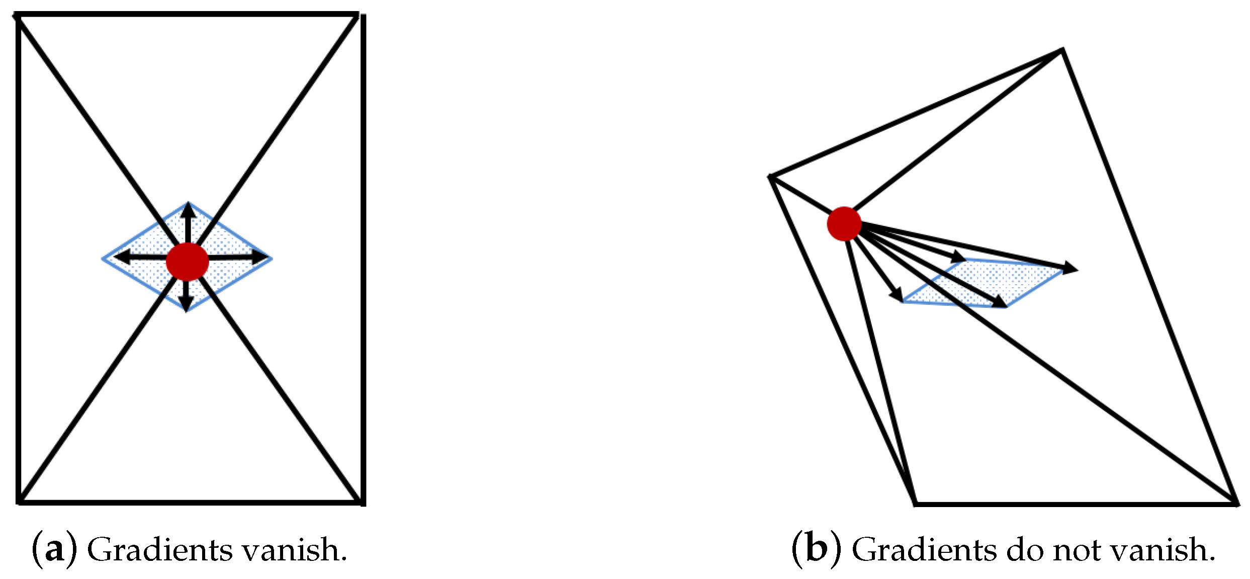
Figure 1a shows an example when the gradient of the constituent element quality with respect to the free vertex (red) vanishes. The four arrows indicate the (negative) gradient of their quality with respect to the free vertex. Since our goal is to minimize the objective function as in Equation (2), we consider the direction of the negative gradients. The blue area indicates a convex hull of the gradients, and the free vertex is located inside the convex hull of the gradients. For this case, the gradients vanish since all elements around the free vertex reach the ideal element qualities. Therefore, the movement of the free vertex could deteriorate the element qualities (of at least one element) around the free vertex. Figure 1b shows an example when the free vertex is located outside the convex hull of the (negative) gradients of the constituent element quality functions. For this case, the movement of the free vertex is able to significantly improve all element qualities around the free vertex. Therefore, we prioritize this free vertex when the vertex reordering is performed.

4. Algorithm

4.1. Vertex Reordering Algorithm

Based on our previous observation, our objective function is optimal when two or more elements have the same quality and the gradients of the function defining their quality are directed such that their convex combination can vanish, i.e., there is a convex combination of the gradients of the worst quality elements whose magnitude is zero. If such a combination exists, we will call them suitably directed gradients.

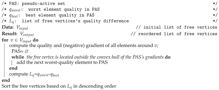
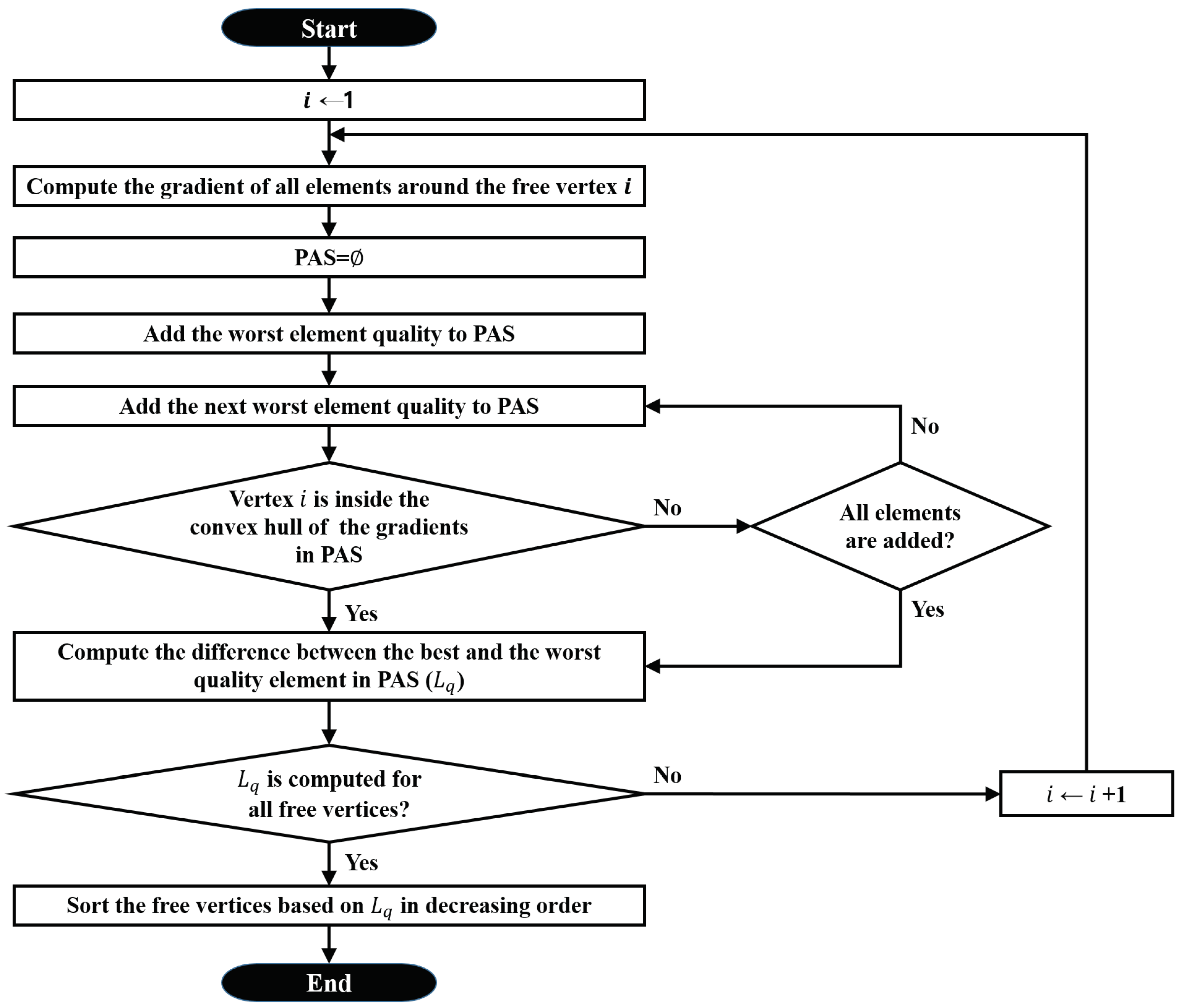
To compute the ordering of free vertices, we first sort our elements based on their quality by descending order and compute the gradient of their quality with respect to the free vertex. Second, for every free vertex, we start with the worst-quality element and add other elements to this “pseudo-active” set (PAS) until the gradients of the function defining their qualities are suitably directed such that their convex combination of gradients can vanish. Specifically, we add the next worst-quality element to PAS until the free vertex is inside the convex hull of the gradients. Third, we compute the difference in the quality of the best ($q_{best}$) and the worst-quality ($q_{worst}$) element in the PAS for every free vertex. Finally, we sort the vertices based on the difference in the quality ($L_q$) in descending order, where $L_q$ is computed as $q_{worst}$-$q_{best}$. The flowchart and the pseudo code of our algorithm are presented in Figure 2 and Algorithm 1, respectively.

Algorithm 1 Vertex Reordering Algorithm

A high inequality in the quality of elements around a vertex indicates a high potential for quality improvement around the vertex. Thus, our idea is to prioritize the free vertex with large differences between the best and the worst-quality element (i.e., $L_q$), in the pseudo-active set. Optimizing these free vertices is able to quickly improve the mesh qualities and accelerates the mesh optimization process over the entire mesh.

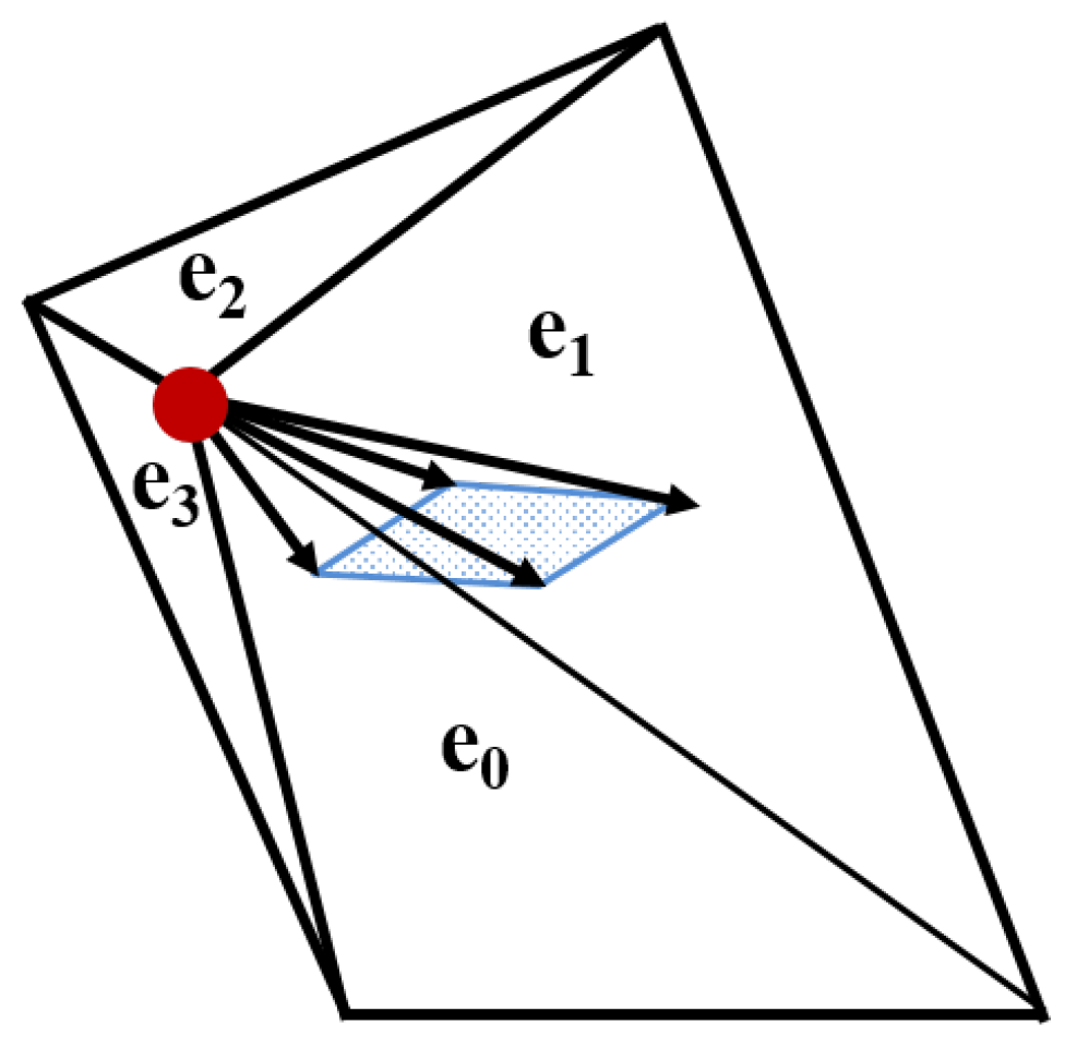
Figure 3 shows a toy example of computing the difference in the quality of the best and the worst element (i.e., $L_q$) in the pseudo-active set for one free vertex. Let the element qualities of four elements, $e_0$, $e_1$, $e_2$, $e_3$, be 1.159, 1.058, 2.064, and 2.911, respectively. A smaller value indicates a better element quality. The four arrows in this figure indicate the (negative) gradient of their quality with respect to the free vertex (red). The free vertex is located outside the convex hull of the gradients of the constituent element quality functions. For this free vertex, $PAS=\left\{e_0,e_1,e_2,e_3\right\}$ and $q_{worst}$ is 2.911 and $q_{best}$ is 1.058, respectively. Finally, $L_q$ is 1.853, which is computed as $q_{worst}$-$q_{best}$. We repeat this process for the other free vertices and sort the free vertices based on $L_q$.

4.2. Mesh Quality Improvement

We focus on improving the worst element quality on the mesh using mesh optimization. Here, mesh optimization refers to a technique of moving interior vertices while fixing the element connectivity. We use local mesh optimization where only one free (interior) vertices moves at a time.

The inverse mean ratio (IMR) quality metric is used to improve the mesh quality [14]. Let a, b, and c be the three vertices of a triangle. Next, define the incidence matrix A by $\left[b-a,c-a\right]$. Let W be the incidence matrix for an ideal element. Then, the IMR quality metric is defined as

$$q(x_i)=\frac{{∥A{W}^{-1}∥}_F^2}{2\left|\det (A{W}^{-1})\right|},$$

(3)

where ${∥·∥}_F$ is the Frobenius norm. The IMR quality metric ranges from 1 to ∞ for valid elements with 1 being the best value.

Since the objective function defined in Equation (2) is a non-smooth objective function, we use a downhill simplex method to minimize it. The downhill simplex method is a popular derivative-free method, which does not use either function derivatives or a Hessian, but only uses function evaluations [15]. It first generates a virtual initial simplex to begin, which is a triangle in 2D and removes the vertex with the worst function value and replace it with another point with a better value by repeatedly performing three actions to find the optimal point: expansions, reflections, and contractions [16]. Readers refer to [15,16] for more details on the downhill simplex method.

When the downhill simplex method is used, initial simplex diameter should be appropriately chosen such that the mesh optimization process converges quickly. Based on the observation in [15], we choose an initial simplex diameter to be 0.1× (minimum edge length).

5. Vertex Reordering Schemes

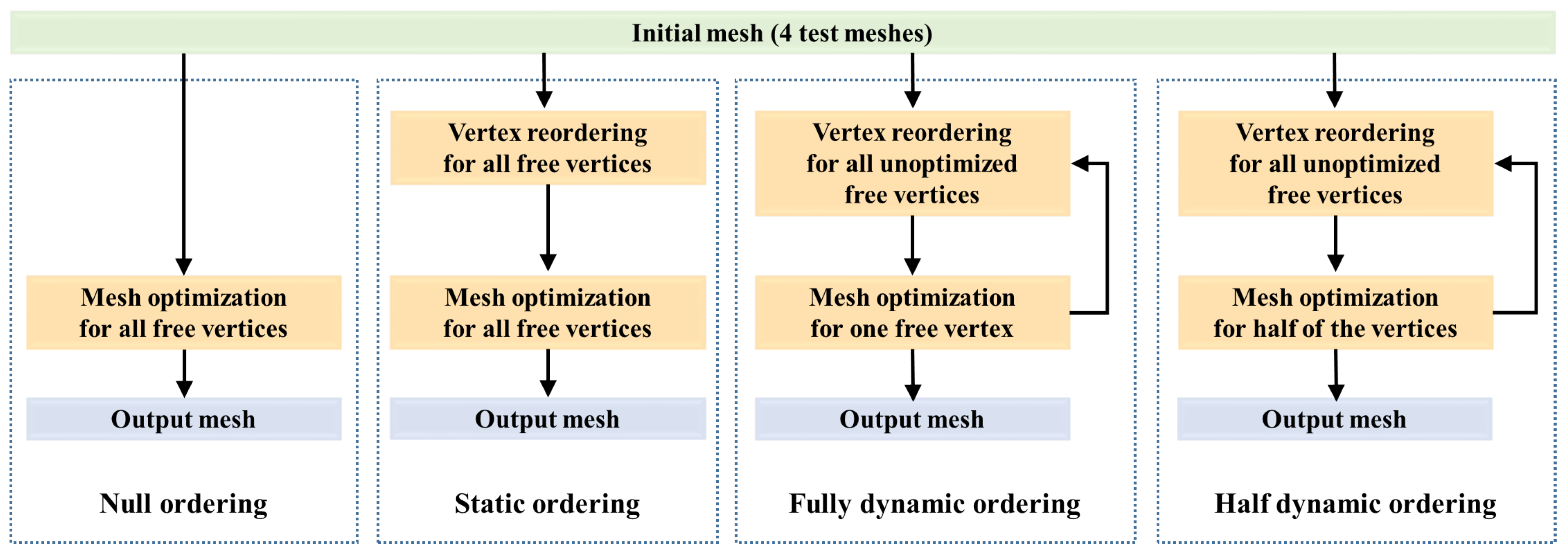
During the mesh optimization process, vertex reordering can be performed either statically or dynamically [10]. For the static case, vertex ordering is performed only once at the beginning of the optimization process, and the ordering remains fixed for all remaining iterations. For the dynamic case, we first reorder the free vertices at the beginning of the optimization process and reapply vertex reordering at the end of some constant number of iterations within the optimization. We further divide dynamic vertex reordering into two methods by how often the reordered list is updated. The fully dynamic ordering updates the reordered list at the end of each iteration within the optimization. The half dynamic ordering is a compromise between a static and fully dynamic vertex ordering. The half dynamic ordering applies vertex reordering at the beginning of the optimization process and updates the reordered list after half of the free vertices are optimized.

The half dynamic ordering is devised from the following observations. We apply the local mesh optimization, which is a Gauss-Seidel type mesh optimization. The element quality around each free vertex varies as the mesh optimization process proceeds. The half dynamic ordering scheme utilizes the updated element quality and performs vertex reordering one more time in the middle of the mesh optimization process. Specific vertex reordering schemes considered in this study are summarized next.

• Null ordering. Do not reorder the free vertices. The ordering is the initial ordering of the free vertices as given by the mesh generator.
• Static ordering. Apply the proposed vertex reordering algorithm at the beginning of the optimization process, and the ordering remains fixed for all iterations.
• Fully dynamic ordering. Apply the proposed vertex reordering algorithm at the end of each iteration within the optimization.
• Half dynamic ordering. Apply the proposed vertex reordering algorithm at the beginning of the optimization process and reapply vertex reordering algorithm after half of the free vertices are optimized.

6. Numerical Experiments

We describe our numerical results to show the effectiveness of the proposed vertex reordering algorithm. Figure 4 summarizes the vertex reordering schemes we used for the numerical experiments. We implemented our vertex reordering algorithms in Mesquite software [17]. Specifically, we used Mesquite version 2.99. A quick sort algorithm was used to perform vertex reordering. The machine employed for this study was equipped with an AMD Opteron processor 6174 (2.2GHz) and 6.5 GB of RAM.

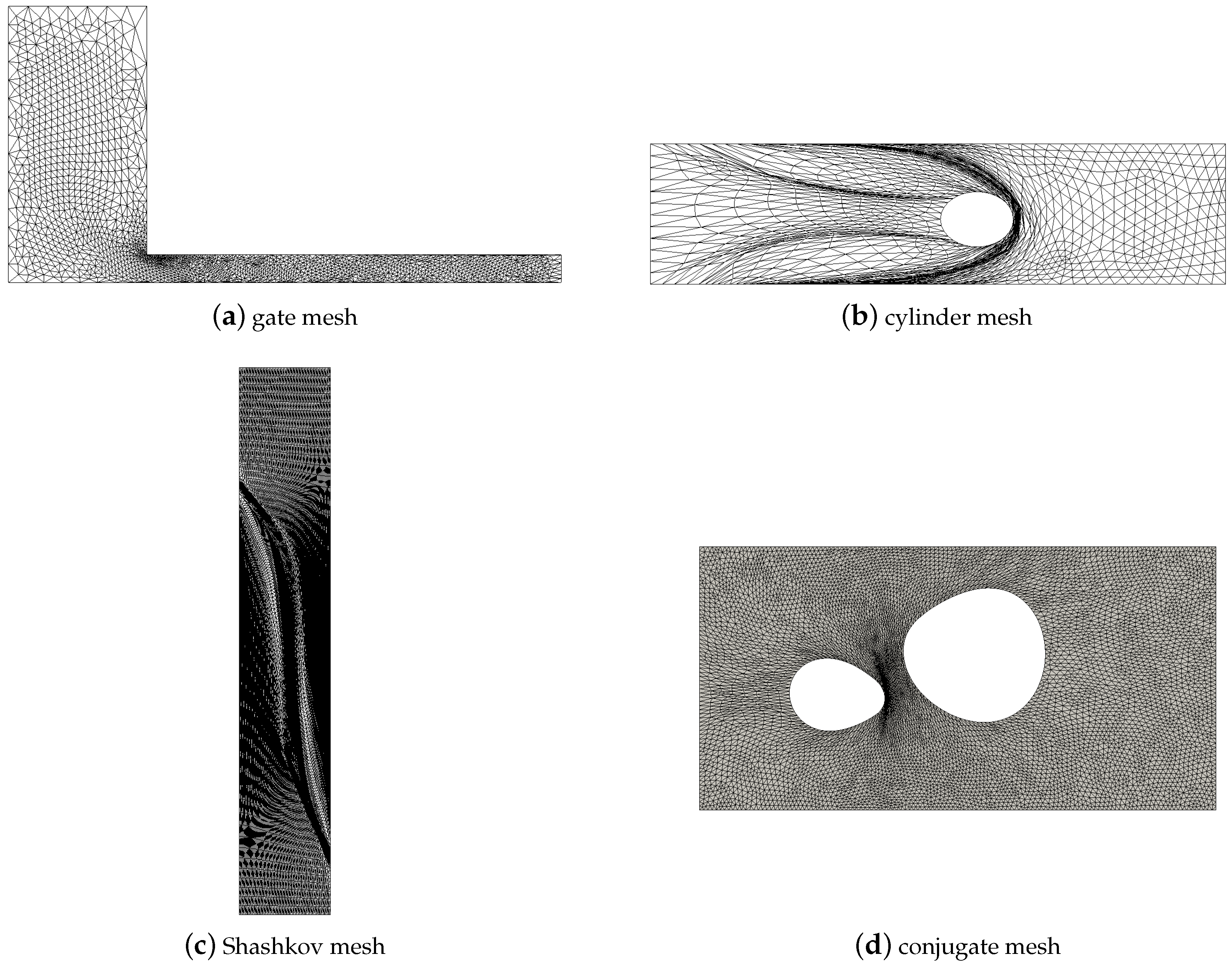
A total of four 2D test meshes, which were triangular, were used as shown in Figure 5. Three meshes (i.e., conjugate, cylinder, gate) were produced during the mesh deformation process and the Shashkov mesh was provided in Mesquite software. Properties of the four test meshes and mesh quality statistics (minimum, average, maximum and standard deviation) are shown in

Table 1. The test mesh configurations.

Mesh Name	# of Vertices	# of Elements
Gate	2107	4034
Cylinder	4167	7232
Shashkov	5252	10,200
Conjugate	6994	13,441

and

Table 2. Mesh quality statistics.

Mesh Name	Min	Avg	Max	Std.dev
Gate	1.001	1.737	87.152	5.355
Cylinder	1.000	12.315	2282.600	53.123
Shashkov	1.000	13.213	277.046	21.821
Conjugate	1.000	1.404	30.992	1.201

, respectively. The IMR quality metric was used to measure the element quality. A smaller value indicated a better element quality, and the ideal element had a value of one. We also tested the proposed vertex reordering schemes using other shape-based mesh quality metrics such as a condition number quality metric [17]. Due to the page limits, those results were omitted here but we observed consistent results. We performed an accurate mesh optimization such that the mesh optimization procedure is driven to a highly converged solution [2].

6.1. Mesh Quality

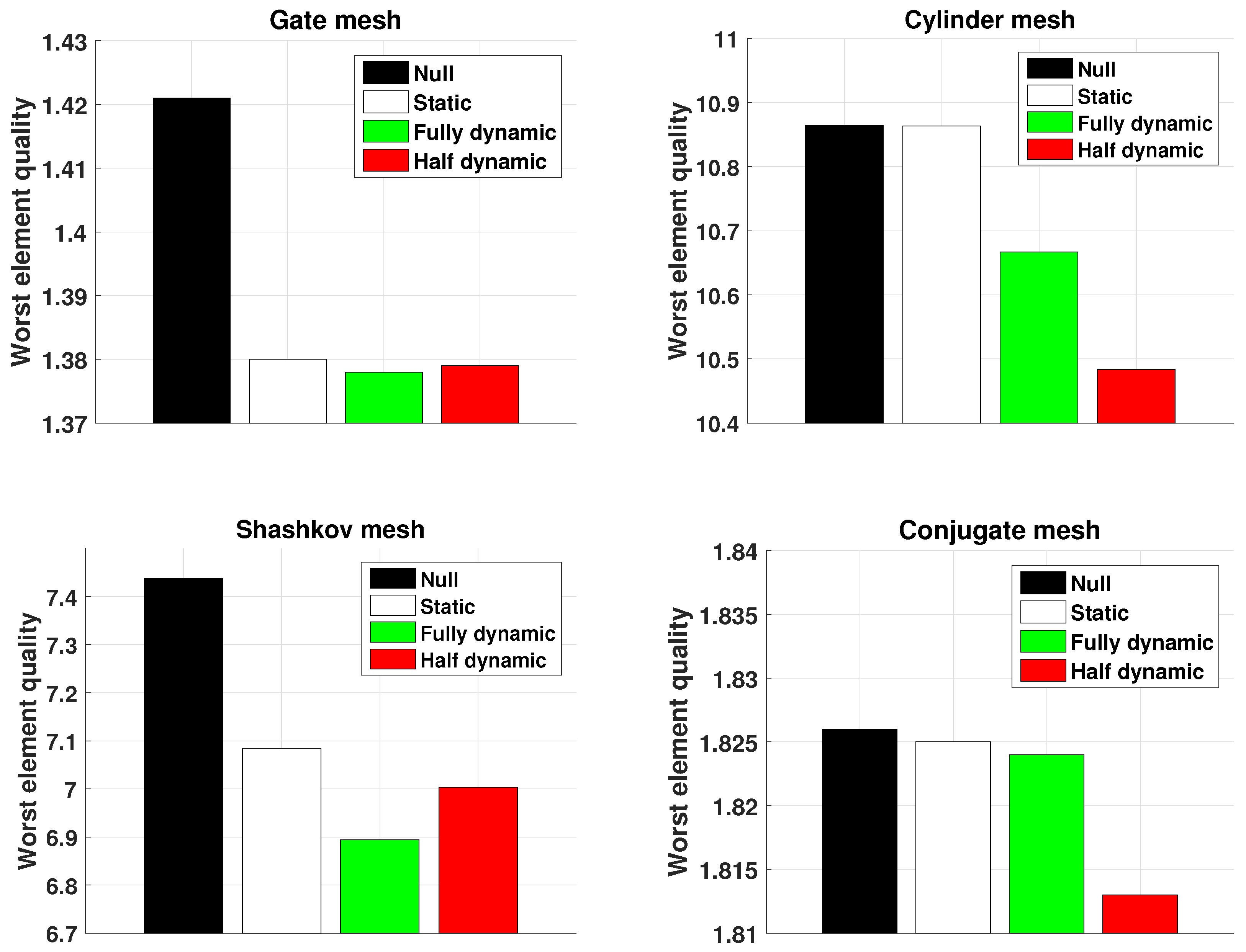
The purpose of this experiment was to observe whether the proposed vertex reordering techniques are able to improve the element quality compared with the null ordering technique, which does not reorder free vertices. Figure 6 shows the worst element quality on the optimized test meshes using various vertex reordering methods. For all test cases, the proposed vertex reordering techniques outperformed the null ordering technique. We observed that the proposed vertex reordering techniques improve the worst element quality up to 7.3% compared to those with the null ordering method.

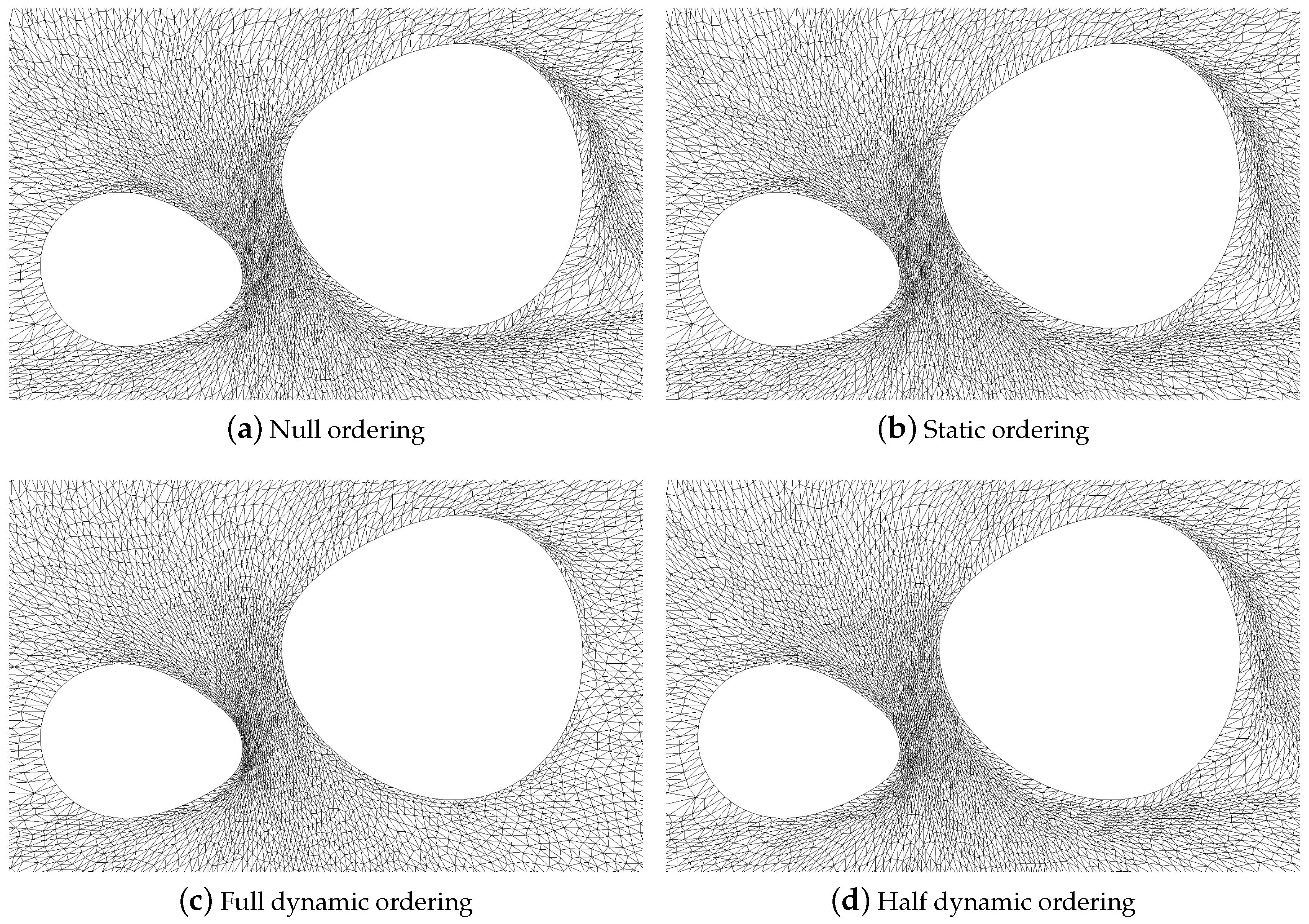
Figure 7 shows the optimized output meshes when various vertex reordering techniques are used for the conjugate mesh. In terms of the worst element quality, the half dynamic vertex reordering technique produces the best output mesh. The worst element quality was 1.813 when the IMR quality metric was used. Figure 7 shows that the output mesh using the full dynamic vertex ordering for the conjugate mesh. The output mesh using the full dynamic vertex ordering method shows better average element qualities compared with the output meshes using other vertex reordering techniques. For this output mesh with the dynamic vertex ordering, we observed that the triangular elements are more uniform and close to equilateral triangles. 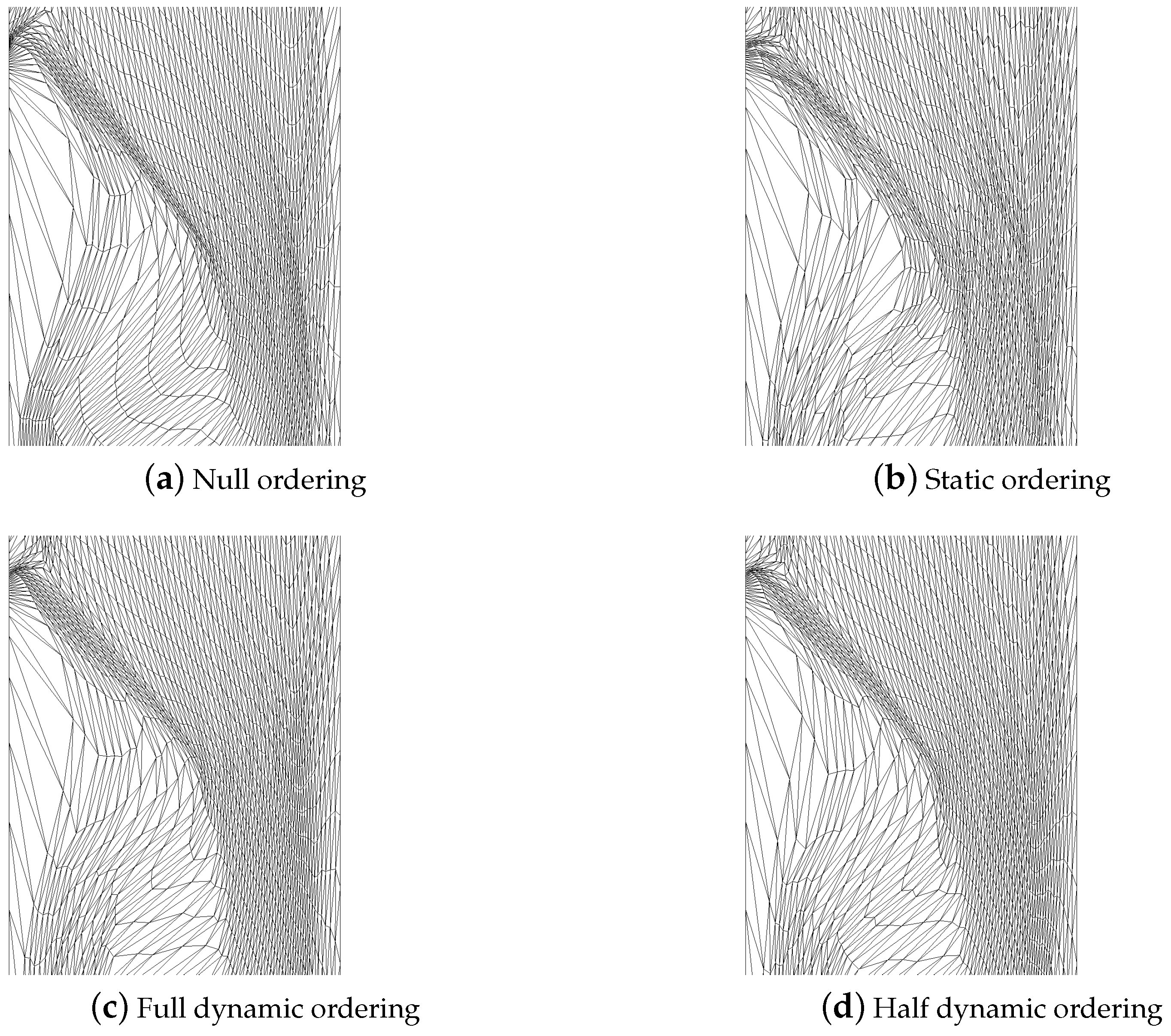Figure 8 shows the optimized output meshes when various vertex reordering techniques are used for the Shashkov mesh. The fully dynamic vertex ordering technique also produces the best output meshes in terms of both the worst and average element qualities.

Table 3. $L_q$ value distributions for initial meshes.

Mesh Name	Min	Avg	Max	Std.dev
Gate	0.002	1.292	84.863	7.437
Cylinder	0.001	11.934	2270.890	74.233
Shashkov	0.001	6.836	225.536	18.374
Conjugate	0.001	0.246	20.975	0.695

shows initial $L_q$ value distributions for various meshes. For the cylinder and Shashkov meshes, the deviation (also, the maximum) of $L_q$ values are larger than the gate and conjugate meshes. It indicates that the cylinder and Shashkov meshes are more heterogeneous compared to the other two meshes. Our previous results show that the proposed vertex reordering techniques are more effective for non-uniform meshes whose maximum and the standard deviation of the $L_q$ values are large. This is because the proposed vertex reordering technique utilizes the difference in the quality of the best and the worst element (i.e., $L_q$) in the pseudo-active set.

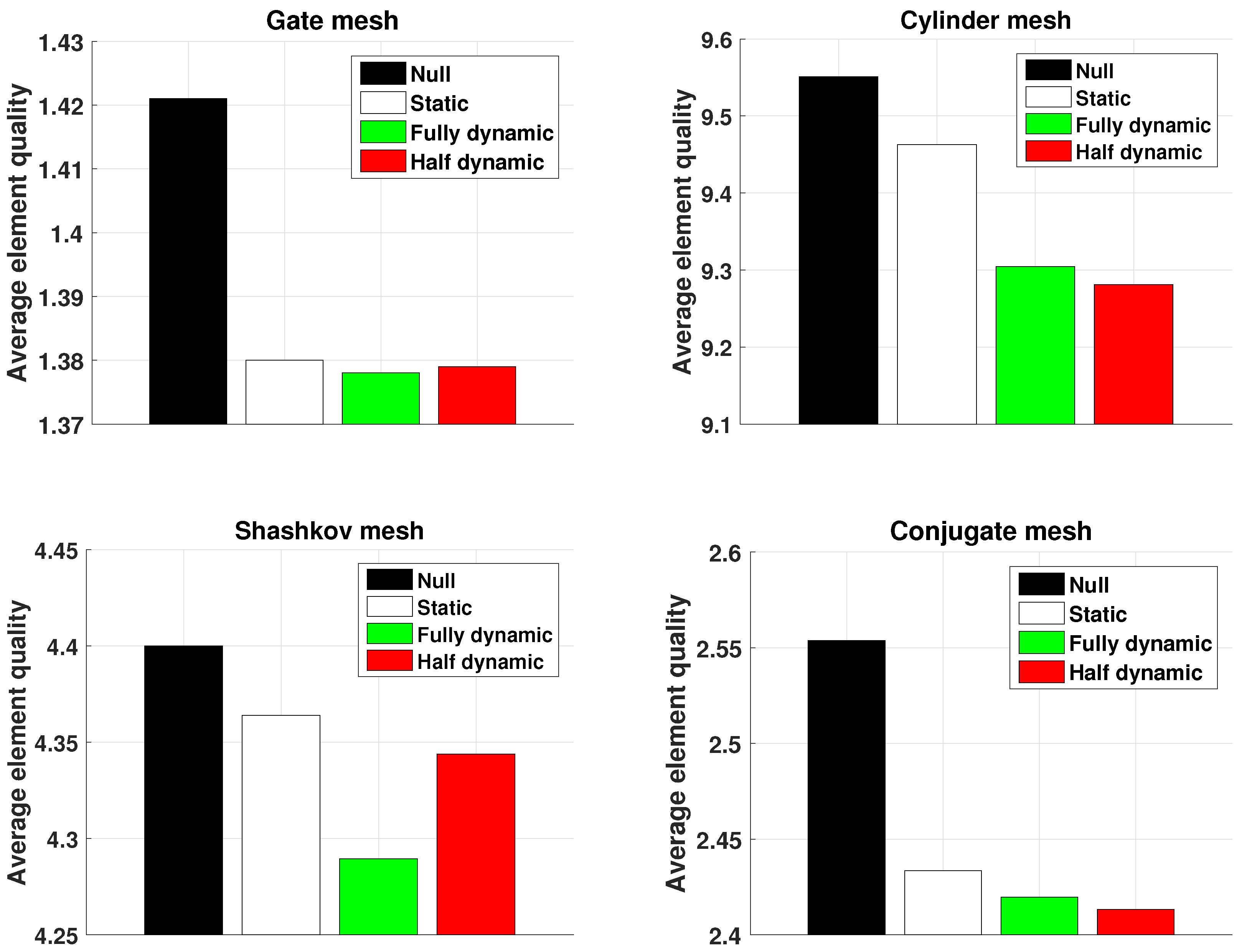
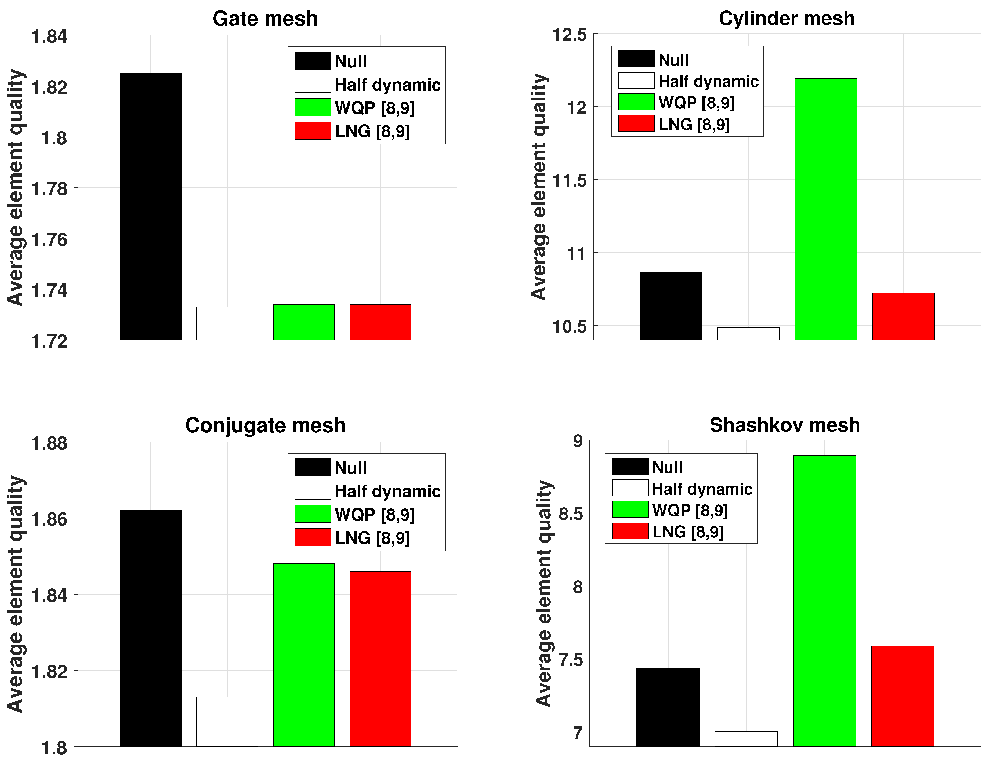
We also investigated whether the proposed vertex reordering techniques were able to also improve the average element quality on the mesh. Figure 9 shows the average element quality on the optimized test meshes using various vertex reordering methods. For all test meshes, the proposed vertex reordering methods outperformed the null reordering method, which does not perform vertex reordering. The average element quality is improved by up to 5.5% when the proposed vertex reordering techniques are used compared with the one with the null vertex reordering. Therefore, the proposed vertex reordering techniques was able to simultaneously improve both the worst and average element qualities.

6.2. Timing

The purpose of this experiment is to observe the effect of the vertex reordering on the CPU time. Here, the CPU time means the total time, which includes both the vertex reordering time and the mesh optimization time. The null ordering method only includes the mesh optimization time, but other vertex reordering methods take additional vertex reordering time.

Table 4. Timing results (gate mesh).

Reordering Schemes	Reordering Time	Optimization Time	Total Time
Null ordering	-	99.365	99.365
Static ordering	0.600	70.511	71.111
Fully dynamic ordering	1388.830	53.839	1442.669
Half dynamic ordering	2.145	64.465	66.609

,

Table 5. Timing results (cylinder mesh).

Reordering Schemes	Reordering Time	Optimization Time	Total Time
Null ordering	-	86.144	86.144
Static ordering	0.003	71.294	71.297
Fully dynamic ordering	762.746	61.204	823.94
Half dynamic ordering	1.260	54.670	55.930

,

Table 6. Timing results (Shashkov mesh).

Reordering Schemes	Reordering Time	Optimization Time	Total Time
Null ordering	-	136.836	136.836
Static ordering	0.010	141.595	141.605
Fully dynamic ordering	5364.980	107.709	5472.689
Half dynamic ordering	3.168	99.822	102.990

and

Table 7. Timing results (conjugate mesh).

Reordering Schemes	Reordering Time	Optimization Time	Total Time
Null ordering	-	888.510	888.510
Static ordering	0.190	1028.149	1028.339
Fully dynamic ordering	9971.850	96.021	10,067.871
Half dynamic ordering	32.533	983.007	1015.540

show comparisons of the vertex reordering time, mesh optimization time and the total time using various vertex reordering methods.

For all tested meshes, the fully dynamic vertex reordering method is the slowest among the compared methods since it updates the vertex list at the end of each iteration. Surprisingly, the half dynamic vertex reordering method takes less total time than the null reordering scheme for all tested meshes other than the conjugate mesh. These results can be understood by two factors. First, the vertex list is only updated at the beginning of the optimization process and after half of the vertices are optimized. Therefore, the computational overhead for sorting is small. Second, due to the smart vertex reordering, free vertices are quickly converged to the optimal locations and the mesh optimization timing is minimized. Overall, the half vertex reordering method shows the best performance in most cases when considering both mesh quality and timing. It simultaneously improves both the average and worst element quality with the minimal computational overhead.

6.3. Comparison with Existing Vertex Reordering Schemes

We compare the proposed vertex reordering schemes with the existing vertex reordering methods in terms of both the worst element quality and the timing. Specifically, we compared the proposed half dynamic vertex reordering method with two existing static vertex reordering schemes. We chose the half dynamic vertex reordering scheme for comparison among the proposed vertex reordering techniques, since our numerical results show robust performance for both mesh quality and timing. The full dynamic vertex reordering scheme was too slow to use in practice for large size meshes.

First, the existing vertex reordering method was a WQP (worst quality patch) method, which orders the free vertices from worst quality first, and the best quality last [10,11]. The second method is the LNG (largest norm of gradient) method, which evaluates the $l_2$ norm of the local gradient of the objective function and sorts the free vertices by putting the largest norm first, and the smallest norm last [10,11]. Our preliminary results show that the dynamic version of both LNG and WQP are too slow to converge. Therefore, we compared the proposed half dynamic vertex reordering method with the static version of both LNG and WQP.

For tested meshes, the proposed half dynamic vertex reordering method shows the best performance in terms of the worst element quality on the optimized meshes. Similar results are observed for the average element quality. Both WQP and LNG methods show mixed results. They sometimes improve the worst element quality compared with the null reordering method, but for some test cases, they show poor performance that is worse than the null reordering method. Figure 10 shows the worst element quality of the optimized meshes. For two tested meshes, we observe that the WQP method shows poor performance that is and even worse than the null reordering method. The LNG method showed worse performance than the null reordering method for the Shashkov mesh.

7. Conclusions

We have proposed a novel vertex reordering technique for 2D mesh quality improvement such that the propagation of inequality in the quality of mesh elements is accelerated. Our idea is to prioritize the free vertex with large differences between the best and the worst-quality element, in the pseudo-active set.

Numerical results show that the optimized meshes using the proposed vertex reordering methods improve both the worst and average element quality up to 7.3% and 5.5%, respectively, compared those with the null ordering method, which does not reorder vertices. Moreover, the worst element quality is improved up to 21.3% compared with existing vertex reordering techniques. For some test meshes, the proposed vertex reordering method is able to improve the mesh optimization efficiency up to 31.2% compared with the null ordering method, since free vertices are quickly converged to the optimal points and the mesh optimization time is minimized.

The proposed vertex reordering technique is more effective when the deviation of free vertices’s quality difference (i.e., $L_q$ value) is huge. For such non-uniform meshes, the ordering of vertices is important when the mesh optimization is performed. Among the proposed vertex reordering techniques, we recommend employing the half dynamic vertex reordering method since it shows the best performance in most cases when considering both the output mesh quality and the timing. The full dynamic vertex reordering scheme is too slow to use in practice for large size meshes.

The proposed vertex reordering techniques can be extended to high order meshes. We plan to apply the proposed vertex reordering techniques to improve high order elements. We also plan to extend the proposed vertex reordering method to 3D meshes.