Neighbor Discovery Optimization for Big Data Analysis in Low-Power, Low-Cost Communication Networks

Abstract

Big data analysis generally consists of the gathering and processing of raw data and producing meaningful information from this data. These days, large collections of sensors, smart phones, and electronic devices are all connected in the network. One of the primary features of these devices is low-power consumption and low cost. Power consumption is one of the important research concerns in low-power, low-cost communication networks such as sensor networks. A primary feature of sensor networks is a distributed and autonomous system. Therefore, all network devices in this type of network maintain the network connectivity by themselves using limited energy resources. When they are deployed in the area of interest, the first step for neighbor discovery involves the identification of neighboring nodes for connection and communication. Most wireless sensors utilize a power-saving mechanism by powering on the system if it is off, and vice versa. The neighbor discovery process becomes a power-consuming task if two neighboring nodes do not know when their partner wakes up and sleeps. In this paper, we consider the optimization of the neighbor discovery to reduce the power consumption in wireless sensor networks and propose an energy-efficient neighbor discovery scheme by adapting symmetric block designs, combining block designs, and utilizing the concept of activating nodes based on the multiples of a specific number. The performance evaluation demonstrates that the proposed neighbor discovery algorithm outperforms other competitive approaches by analyzing the wasted awakening slots numerically.

1. Introduction

Connectivity is expected to be one of the most important factors to be considered in the near future. Many electronic devices, such as computers, smart phones, and tablet PCs are connected to each other through the internet nowadays. Even different types of home appliances are connected through internet services. Consequently, significant amounts of information are exchanged every day in the world. Gartner, Inc. estimated that the number of connected devices would reach 20.4 billion by 2020 in a report. It is not easy to imagine the amount of information that would be produced, processed, and exchanged among these devices.

Big data analysis usually requires significant computing and electric power owing to the large amounts of data that have to be processed. Especially, energy consumption is one of the most critical issues for the purpose of information gathering for big data analysis among resource constrained devices, such as wireless or mobile sensors. These machines are both the primary components of low-power and low-cost communication networks and a raw data source used for big data analysis. Hence, it is possible to maintain network connectivity by saving the energy utilized by machines. It is known that communication cost is significantly more expensive than other costs, such as those for collecting or processing information.

As the internet of things (IoT) technology has emerged and has been extensively applied to a variety of areas, several mobile network studies are focusing on low-power, low-cost communication networks [1,2,3,4]. A typical network of low-power communication is a wireless sensor network (WSN). There is no permanent power source in this type of network. Therefore, energy-efficient communication is much more important than other research subjects. Furthermore, the movement of networked devices may frequently occur in mobile networks. Finally, the nodes in these network environments have certain constraints of computing resources and depend on limited electrical power.

It is widely known that IoT communication networks are in general composed of heterogeneous physical devices. Power consumption might not be a significant concern in certain IoT networks; however, low-power consumption and the utilization of wireless devices are considered as an energy-efficient solution. Several IoT communications are based on machine-to-machine (M2M) communication, which is similar to the basic communication method of a wireless sensor network. It is assumed that most sensors do not change their location after they are deployed in the area of interest. However, this assumption might not be applicable to low-power IoT communication networks. For example, sensors that are used in autonomous or unmanned vehicles constantly move during their lifetime. These devices might join and leave the network at any time. Therefore, continuous neighbor discovery should be performed for maintaining network connectivity.

The neighbor discovery process is required to sustain the network connectivity in low-power, low-cost communication networks [5,6,7,8]. Furthermore, this process consumes the battery power of wireless devices. A neighbor discovery optimization problem considers and focuses on how to minimize power consumption as much as possible. In this paper, we propose an energy-efficient neighbor discovery algorithm for symmetric and asymmetric operations. We formulated the neighbor discovery optimization problem with a mathematical term, borrowed the concept of block design in combinatorics for effective neighbor discovery, and analyzed the performance of certain representative neighbor discovery mechanisms numerically.

This paper is configured as follows: Section 2 provides literature reviews of asynchronous neighbor discovery. Section 3 specifies a neighbor discovery optimization process. Section 4 introduces a neighbor discovery problem (NDP), few neighbor discovery schedules, the main features of block designs, and a practical challenge of existing block designs. Section 5 elaborates the primary idea of merging two block designs and focuses on our key contributions. In Section 6, we consider an asymmetric NDP. Section 7 evaluates and measures the performance of the proposed algorithm and compares the proposed scheme with that of other representative neighbor discovery protocols. Finally, we conclude the paper in Section 8.

2. Related Work

Several researchers have conducted studies pertaining to the NDP since this problem was first introduced. Consequently, there are a number of representative outcomes of NDP, referred to as neighbor discovery protocol, in the sensor network research fields. In IoT communication networks, a network topology is constantly updated owing to nodes joining and leaving the network frequently. Consequently, the neighbor discovery process should happen continually to ensure network connectivity. In this section, we present several related works of major neighbor discovery protocols.

The primary idea behind the Birthday protocol [9] follows the birthday paradox in which the birthday of two individuals out of a set of n randomly selected people is the same. This paradox is applied to develop a neighbor discovery protocol in ad hoc networks. Nodes can wake up and sleep with their own probabilities in the network. They merely pursue their probabilities and meet each other at a certain time owing to the paradox. This mechanism is likely to sound advantageous for neighbor discovery. However, it is known that a randomness approach, such as the Birthday protocol, performs well in average cases, but it cannot guarantee neighbor discovery at a worst case. Neighbor discovery should be assured in both average and worst cases with minimum energy consumption.

Each wireless node can randomly choose one row and one column of a two-dimensional array n × n in a Quorum-based neighbor discovery protocol [10,11] for ad hoc networks. Every node activates all the slots from the selected rows and columns and the remaining slots are inactive for neighbor discovery. Consequently, $\frac{2n-1}{n^2}$ slots remain awake and attempt to locate their neighbors at the awakening time. The Quorum-based neighbor discovery protocol can guarantee that two neighbor nodes can identify each other quickly if the two nodes choose the same row or column. Even if this aspect demonstrates the advantage of the Quorum-based protocol, the performance of the protocol depends on which row and column are chosen. Furthermore, we cannot ensure that two different nodes will always select the same row or column.

There are two similar approaches to neighbor discovery that adopts prime numbers: Disco [12] and U-Connect [13]. In Disco, every node chooses two different prime numbers and activates the nodes that are multiples of these numbers to identify if there are neighboring nodes in the communication boundary. The main concept of Disco ensures that there is at least one common time slot between two neighboring nodes at the time of the multiplication of the chosen prime numbers. When compared to previous protocols for neighbor discovery, Disco has its own distinct feature where two nodes are able to locate each other at different duty cycles. The study emphasizes that Disco can support an asymmetric duty cycle. The performance of Disco depends on choosing balanced primes (the difference between two prime numbers of each node is minimal) at a given duty cycle. Choosing two well-balanced prime numbers may not be easy because there is no proper algorithm or formula for identifying balanced prime numbers.

The other neighbor discovery protocol using a prime number is U-Connect [13]. Only one prime number is used in U-Connect instead of using two prime numbers. Unfortunately, there may be no overlap between two neighboring nodes with one prime number. U-Connect activates certain number of slots to overcome the problem of non-rendezvous slots. For instance, $\frac{p+1}{2}$ consecutive slots wake up in the beginning of the time slots per p² slots when a prime number p is selected for neighbor discovery. One of valuable contributions of U-Connect is the performance metric of neighbor discovery protocols called the power-latency (PL) product. U-Connect offers an alternative approach to Disco by using one prime number; however, it still demonstrates a weakness where two nodes are not likely to meet each other quickly in case of a mismatch during the early time slots of a neighbor discovery schedule. This shortcoming may result in a significant increase in the worst-case discovery latency.

The concept of a block design in combinatorial mathematics was used for inventing a neighbor discovery protocol by Zheng et al. [14]. The neighbor discovery schedule can be easily generated using a certain duty cycle from an existing and well-known block design. The combinatorial approach demonstrates the fastest discovery latency and lowest energy consumption when compared to other existing neighbor discovery protocols based on the PL product. It is to be noted that the combinatorial scheme performs well in a situation where all nodes follow the same duty cycle (a symmetric case). However, it may be impossible to apply this approach to an asymmetric case of neighbor discovery. In addition, it is impossible to create a discovery schedule using the concept of the block design if there is no proper set of block designs at a given duty cycle.

The simplest solution of neighbor discovery is to maintain all slots as active until two neighboring nodes identify each other. However, this approach is not applicable to low-power and resource-constrained network environments. Activating half of the total slots in each duty cycle could be a better solution than the previously mentioned extreme one. However, this solution is also not sufficiently good for developing an energy-efficient neighbor discovery protocol. Searchlight [15] offers a clue for energy-efficient neighbor discovery by probing half of the total time slots to determine at least one common active slot. There are two active slots within t contiguous slots: an anchor slot and a probe slot. The anchor slot is the first slot in the discovery period and the probe slot changes its location to search for the anchor slot of the other node. Intuitively, the probing method can reduce the number of active slots marginally; however, the discovery latency takes longer as the total slots in the neighbor discovery period is increased.

Two different types of slots, called static and dynamic slots, are used in BlindDate [16]. The static slot is approximately the same as the anchor slot in Searchlight. The concept of dynamic slot is similar to that of the probe slot of Searchlight; however, the moving directions constantly change from left to right or right to left to locate neighboring nodes quickly. This mechanism can decrease the worst-case discovery latency when compared to Searchlight. However, the performance of BlindDate is only marginally different from that of Searchlight.

3. Problem Statement

There are generally two power-operating modes called sleeping and awakening modes in most energy-saving mechanisms in wireless networks [17,18,19,20,21]. In the sleeping mode, a wireless node turns off its radio interface and expends only a small amount of power, thereby saving energy when it turns on its radio for communication in the awakening mode.

One of the simplest ways to reduce the power consumption of wireless nodes in the network minimizes the number of awakening modes. If the nodes sleep for most of their network lifetime, then we could achieve the optimization of power consumption in wireless sensor networks effectively. Unfortunately, this power management mechanism is ineffective because the entire network remains disconnected. Hence, we are required to accomplish both network connectivity and power management.

As we mentioned before, the power-saving policy consists of the sleeping and awakening modes. Each node might follow its own power management schedule based on its own policy. We can formulate the power management schedule to represent two power-saving modes using a binary number. A binary number “zero” can be used to represent the sleeping mode and the number “one” can express the awakening mode. All the sensor devices that follow this power-saving policy alternate between the sleeping and awakening modes continuously. Therefore, the power management schedule, $\mathcal{S}$, can be illustrated as zero and one. Furthermore, each wireless node has its own duty cycle of a certain length of schedule, $ℒ$. The power management schedule of node u, ${\mathcal{S}}_u$, can be represented by a polynomial of order $ℒ$ as

$${\mathcal{S}}_u\left(x\right)={{\displaystyle \sum }}_{i=0}^{ℒ-1}{a}_i{x}^i,$$

(1)

where $ℒ$ is the length of the schedule, $a_i$ = 0 or 1 ($0\le i\le ℒ-1)$, and x is a place holder.

By definition, two nodes, u and v, wake up in slot i if a_i = 1. In this situation, they can communicate with each other if they are within the same communication range; thus, it can be noted that nodes u and v identify their neighbors. Conversely, it may be difficult for them to talk to each other when u is awake and v sleeps at slot i, or vice versa. In the latter scenario, an awakening node cannot avoid wasting its energy and the neighboring nodes u and v are unable to identify each other. For neighbor discovery optimization to achieve low-power, lost-cost communication networks, an ultimate goal is to minimize the number of wasted awakening slots as much as possible during the neighbor discovery process.

By the above definition of $\mathcal{S}$, ${\mathcal{S}}_u\left(1\right)$ is the total number of slots where node u should be awake for neighbor discovery in every $ℒ$ slot when a_i = 1. If we apply a bitwise XOR operation (^) to ${\mathcal{S}}_u\left(x\right)$ and ${\mathcal{S}}_v\left(x\right)$, then it would be possible to determine the number of wasted awakening slots that exist between ${\mathcal{S}}_u\left(x\right)$ and ${\mathcal{S}}_v\left(x\right)$. In addition, we can calculate the number of overlapping awakening slots that occur between ${\mathcal{S}}_u\left(x\right)$ and ${\mathcal{S}}_v\left(x\right)$ if we assign a bitwise AND operation (&) to ${\mathcal{S}}_u\left(x\right)$ and ${\mathcal{S}}_v\left(x\right)$. Let ${\mathcal{S}}_{u^v}\left(1\right)$ be the total number of wasted awakening slots and ${\mathcal{S}}_{u\&v}\left(1\right)$ be the total number of overlapping awakening slots between ${\mathcal{S}}_u\left(x\right)$ and ${\mathcal{S}}_v\left(x\right)$. Therefore, we define a neighbor discovery optimization problem as follows:

$$\begin{array}{c}\mathrm{Minimize}:\hspace{1em}{\mathcal{S}}_{u^v}\left(1\right)\\ \mathrm{Subject}\mathrm{to}:\hspace{1em}{\mathcal{S}}_{u\&v}\left(1\right)\ge 1\end{array}$$

(2)

4. Block Design for Neighbor Discovery

It is crucial to minimize the total number of wasted awakening slots in the neighbor discovery optimization problem. However, fundamentally, two nodes, u and v should locate each other within $ℒ$ slots. Hence, in this section, we introduce a block design for neighbor discovery. The NDP can be applied to the block design in combinatorics theory. Initially, we define certain important terminologies in neighbor discovery.

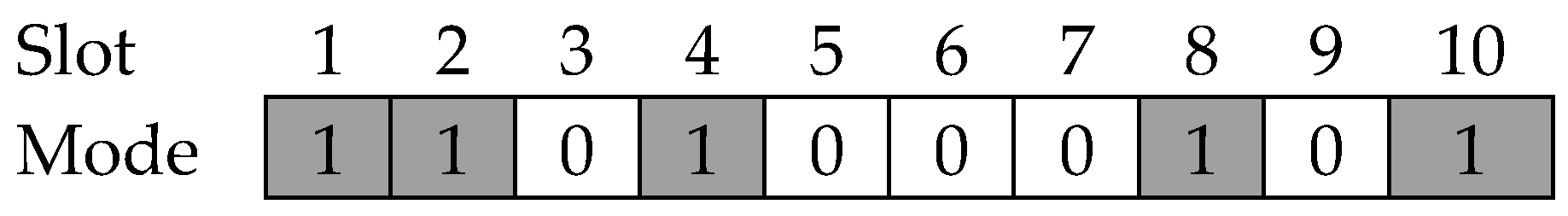
Definition 1.

A discovery schedule (DS) is a repetition of zeroes or ones that represents the sleeping and awakening modes, respectively. When a wireless node is in the awakening mode, it should be scheduled to turn its radio on for communication and prepare to transmit or receive packets. If the node stays in the sleeping mode, then it should turn its radio off and obtain certain environmental information. In a DS, the binary number zero represents the sleeping mode and one denotes the awakening mode.

Definition 2.

A DS consists of a certain number of place holders containing the binary numbers, zero or one. We call this place holder a “slot”. Therefore, each DS has its own number of slots representing sleeping or awakening modes.

Definition 3.

A duty cycle (D) is the ratio of the number of active slots over the total number of slots for a given DS. Therefore, D can be expressed as:

$$\mathrm{D}=\frac{\mathrm{A}}{\mathrm{T}}\times 100\%,$$

where A is the number of awakening slots and T is the total number of slots in a DS. Hence, D illustrates the number of slots that should be awake in a DS.

It is possible to express DS graphically as illustrated in Figure 1. Based on Definition 1, there are only two modes in the DS. Therefore, it can be said that the DS is a sequence of zeroes and ones representing awakening or sleeping slots. Figure 1 shows a typical example of a DS. In this example, the DS consists of 10 slots and the duty cycle of the DS is $\frac{5}{10}\times 100\%=50\%$.

We adapted the basic idea of the block design to address the NDP. The block design is defined as follows [22,23,24]:

Definition 4.

A design is a pair (X, A) such that the following criteria are satisfied:

(1) 

X is a set of elements (points), and

(2) 

A is a collection of non-empty subsets of X (blocks).

Definition 5.

Let v, k, and λ be positive integers such that v > k ≥ 2. A (v, k, λ)-balanced incomplete block design ((v, k, λ)-BIBD) satisfies the following properties:

(1) 

|X| = v,

(2) 

Each block has exactly k points, and

(3) 

Every pair of distinct points is included in exactly λ blocks.

Thus, (7, 3, 1)-BIBD is one of the representative BIBDs when λ = 1. In the (7, 3, 1)-BIBD,

X = {1, 2, 3, 4, 5, 6, 7}, and
A = {{1,2,4}, {2,3,5}, {3,4,6},
{4,5,7}, {5,6,1}, {6,7,2}, {7,1,3}}.

In (7,3,1)-BIBD, each block is composed of three points and each pair of distinct points is exactly related to one block. For example, a block {1,2,4} contains elements 1, 2, and 4 and a pair (2,3) or (3,5) only appears in a block {2,3,5}.

In the theory of block design, if the number of blocks is the same as the number of points, i.e., |X| = |A|, then they call this design a symmetric-BIBD. In Reference [25], based on Theorem 1.2.1, it was discussed that if a block design is a symmetric-BIBD, then the arbitrarily chosen two blocks have λ common points. This theorem involves a basic property where two random DSs might have overlapping awakening slots when applying the symmetric-BIBD to the NDP. Therefore, we introduce this theorem here.

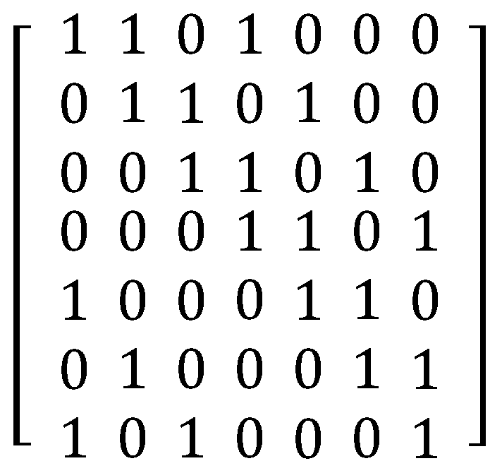
Theorem 1.

(Theorem 1.2.1 in [25]): If (X, A) is a symmetric-BIBD with parameters (v, k, λ), any two different blocks have exactly λ common points.

It is possible to rewrite all the blocks in (7,3,1)-BIBD. For instance, a block {1,2,4} can be replaced by (1101000) with binary numbers, zero and one. The (7, 3, 1)-BIBD can be demonstrated explicitly as shown in Figure 2 using the notation of a matrix. This binary matrix of blocks completely corresponds with the design of DS. Hence, we can allocate one of the blocks to each wireless node at random as its own DS.

This ensures that the symmetric-BIBD guarantees at least one overlapping awakening slot between two DSs for neighbor discovery. Theorem 2 demonstrates that any arbitrary two DSs have λ overlapping awakening slots when we employ symmetric-BIBD to the design of DSs.

Theorem 2.

If two distinct DSs, S_i and S_j, are applied to the (X, A) symmetric-BIBD with parameters (v, k, λ), then the two DSs, S_i and S_j, have λ overlapping awakening slots.

Proof: 

As (X, A) is a symmetric-BIBD with parameters (v, k, λ), X and A can be represented as follows:

X = {p₁, p₂, …, p_v}, and

$$A=\left\{B_i\right|B_i\subset X,\left|B_i\right|=k\}$$

Two schedules, S_i and S_j, can be connected to two distinct blocks in A, respectively. Let two blocks in A be B_i and B_j. According to Theorem 1, there exists λ points in B_i and B_j. Consequently, it is possible to mention that | B_i ∩ B_j | = λ. It shows that S_i and S_j, which are applied to B_i and B_j, respectively, have λ overlapped active slots. □

It is already known that if k is a power of a prime, there exists a block design (k² + k + 1, k + 1, 1)-BIBD for λ = 1; further, this kind of BIBD is a symmetric-BIBD [22]. (7, 3, 1)-BIBD is a case where k = 2. By choosing an appropriate power of the prime k, we would be able to create several DSs with different duty cycles. Although this idea seems as a possible method for designing DSs, there is a practical challenge in adopting a (v, k, 1)-BIBD directly.

The practical challenge of a block design is that there is no algorithmic and well-known block construction method. In a general WSN application, it is required to make a set of DSs with a low duty cycle to save considerable energy of wireless sensors. For maintaining a low duty cycle continuously, a relatively big prime number should be selected to generate a set of blocks. However, a big prime number results in a large number of blocks. Hence, big prime numbers may considerably influence the computational time for generating blocks. It might not be possible to search for a proper BIBD within a constant time when very low duty cycles are required. If we cannot select a suitable block construction technique for a target low duty cycle, we must consider $\left(\begin{array}{c}{k}^2+k+1\\ k+1\end{array}\right)\times \left(\begin{array}{c}{k}^2+k+1\\ 2\end{array}\right)$ number of trials as the worst-case scenario to search all the blocks of a (k² + k + 1, k + 1, 1)-BIBD.

5. Block Construction Mechanism

As we stated in the previous section, a practical challenge results in a difficulty in creating a DS by adopting a symmetric-BIBD directly. A new approach is required for producing neighbor discovery schedules within a small amount of computational time. We have introduced our proposed DS construction mechanism and its specific features in this section.

A fundamental idea of the proposed scheme is mixing two existing block designs and creating a discovery schedule. The symmetric-BIBD is only used to illustrate and explain how our technique is operated.

Definition 6.

Let v, k, and λ be positive integers such that v > k ≥ 2. A (v, k, λ)-neighbor discovery design ((v, k, λ)-NDD) is a design (X, A) such that the following characteristics are valid:

(1) 

|X| = v,

(2) 

Each block has exactly k awakening slots, and

(3) 

Every pair of different blocks includes at least λ common awakening slots.

Definition 7.

A sleep schedule is a n × n matrix with a value of all zeroes.

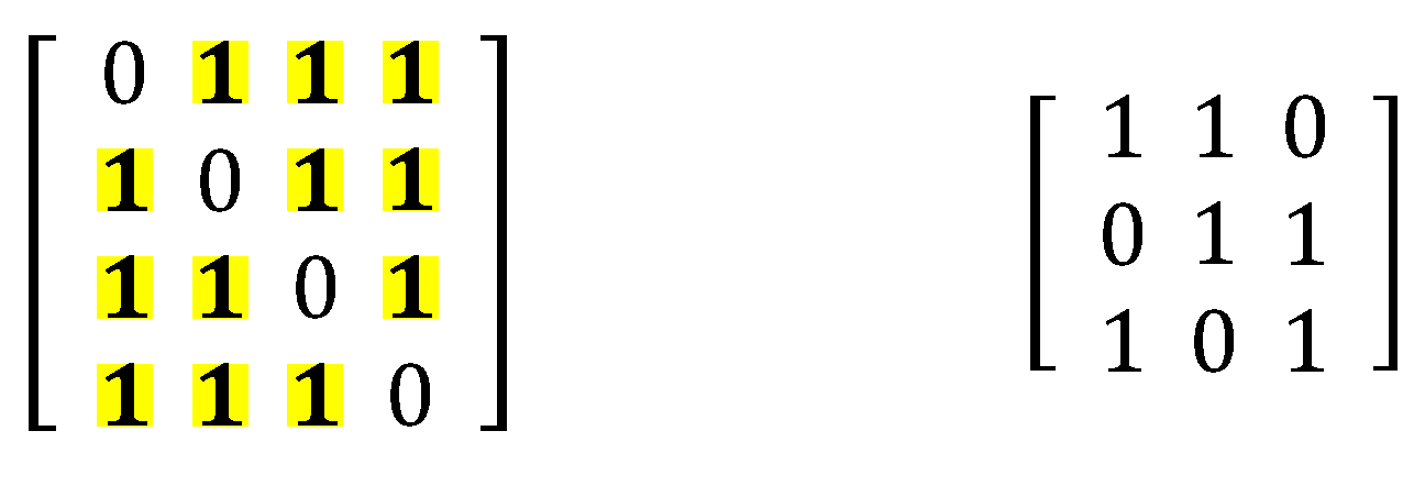
We only created (4,3,2)- and (3,2,1)-designs for the purpose of explaining how to combine two block designs. It is to be noted that these two block designs were constructed only for demonstrating the process of making neighbor discovery schedules.

Step 1: Preparing two block designs.

First, we prepared two well-known block designs. We assumed that there are two block designs: A = (v_a, k_a, λ_a)-BIBD and B = (v_b, k_b, λ_b)-BIBD. (4,3,2)- and (3,2,1)-designs were created to demonstrate the operation of the proposed combining process. The (4,3,2)- and (3,2,1)-designs are shown in Figure 3. We defined the (4, 3, 2)-design as base and the (3,2,1)-design as replacement.

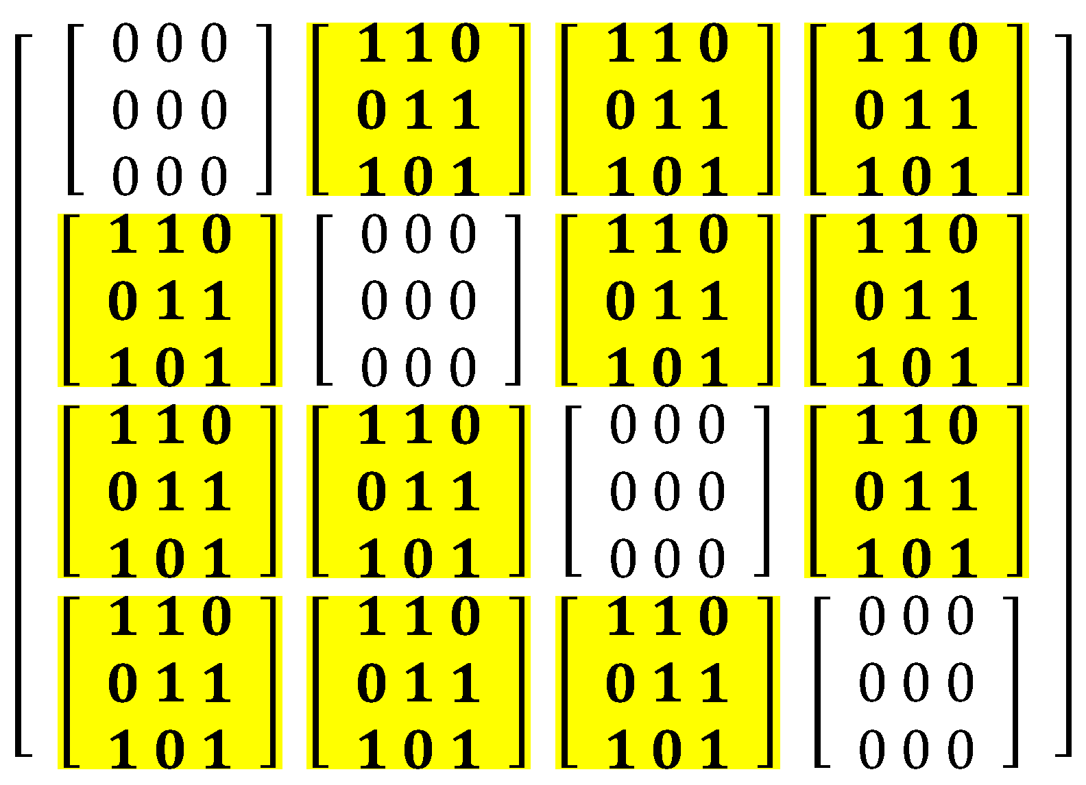
Step 2: Replacing each awakening slot in the base by the entire slot of the replacement.

Secondly, each awakening slot in the base was replaced by the total slots of the replacement. In addition, all sleeping slots were changed into a sleep schedule as per Definition 7. Each awakening slot in the (4,3,2)-design was transformed to entire slots in the (3,2,1)-design.

Step 3: Constructing a new block design.

It is possible to create a (v_a × v_b, k_a × k_b, λ_a × λ_b)-NDD by implementing steps 1 and 2 in the final step. A new block design, (12,6,2)-NDD, is shown in Figure 4. It is finally produced by combining the (4,3,2) and (3,2,1)-designs.

It can be guaranteed that we can produce and create a number of diverse DSs with a target duty cycle by repeating the proposed construction method through steps 1 to 3. If the existing well-known block designs are able to cover the given duty cycle, it could simply use it to construct a neighbor discovery schedule. However, it is not always possible to do that because of the lack of a general algorithm for generating BIBDs. Consequently, the proposed idea can be applied for solving the NDP. As you have seen, it is relatively simple to create a new block design for neighbor discovery. Additionally, our technique is reasonable with respect to the computational time.

It is required to prove that the newly created block design has the same features as specified in Definition 5. The process for proving this is really important and critical. If the new block design does not have the same properties of the original block design, then the new one is inoperable and it cannot be applied to the NDP. The proposed scheme can guarantee that the new DS has the same properties as the original block designs.

Definition 8.

We assumed that F is defined as a (v₁, k₁, 1)-BIBD and $ℛ$ is declared as a (v₂, k₂, 1)-BIBD. F $\otimes ℛ$ represents that all the awakening slots in F are transformed to $ℛ$ and all the sleeping slots are changed into a v₂ $\times$v₂ size matrix of the sleep schedule.

Theorem 3.

We assume that F is a (v₁, k₁, 1)-BIBD and $ℛ$ is a (v₂, k₂, 1)-BIBD. F $\otimes$$ℛ$ results in a (v₁ × v₂, k₁ × k₂, 1)-NDD.

Proof: 

Both F and $ℛ$ are BIBDs. Hence, it is possible to say that F = {${\mathrm{F}}_i$ | ${\mathrm{F}}_i$ is a schedule} and $ℛ$ = {T_i | T_i is a schedule}. We assumed that $\mathsf{\Psi }$ = F $\otimes$ $ℛ$. We know that $\mathsf{\Psi }$ = {${\mathsf{\Psi }}_i$ | 1 $\le$ | ${\mathsf{\Psi }}_i$ | $\le$ v₁v₂} is a (v₃, k₃, 1)-NDD, where v₃ = v₁v₂ and k₃ = k₁k₂. Thus, ${\mathsf{\Psi }}_j$ $\in$ $\mathsf{\Psi },$ where i $\ne$ j, $\exists$ 1 $\le$ h $\le$ v₁v₂ such that $\omega$_ih = $\omega$_jh = 1 for any pair of schedules ${\mathsf{\Psi }}_i$. Every awakening slot in $\mathrm{F}$ is transformed to $ℛ$ by $\mathrm{F}$ ⊗ $ℛ$. In addition, every sleeping slot in $\mathrm{F}$ is changed into a v₂ × v₂ sized matrix of all zeros. Hence, it is possible to express that the total number of points in $\mathsf{\Psi }$ is v₁ × v₂ and each block in $\mathsf{\Psi }$ has exactly k₁ × k₂ awakening slots. These two chrematistics perfectly correspond to the first and second properties in Definition 10. Consequently, we concluded that every pair of differing two blocks has at least λ common awakening slots. $\mathsf{\Psi }$ can be illustrated with the notation of the matrix as follows:

$$\mathsf{\Psi }=\left[\begin{array}{cccc}{\psi }_{(1,1)}& {\psi }_{(1,2)}& \cdots & {\psi }_{(1,v_1{v}_2)}\\ {\psi }_{(2,1)}& {\psi }_{(2,2)}& \cdots & {\psi }_{(2,v_1{v}_2)}\\ ⋮& ⋮& \ddots & ⋮\\ {\psi }_{(v_1{v}_2,1)}& {\psi }_{(v_1{v}_2,2)}& \cdots & {\psi }_{(v_1{v}_2,v_1{v}_2)}\end{array}\right]$$

$\mathsf{\Psi }$ is a v₁v₂ × v₁v₂ sized matrix and each component of $\mathsf{\Psi }$ denotes an awakening or a sleeping slot. Schedules ${\mathsf{\Psi }}_i$ and ${\mathsf{\Psi }}_j$ represent one of the rows in $\mathsf{\Psi }$. $\mathrm{F}$ is a BIBD. Therefore, $\mathrm{F}$ has a schedule ${\mathrm{F}}_i$. Each ${\mathrm{F}}_i$ has at least one awakening slot, s_im, where 1 ≤ m ≤ v₁v₂. According to Definition 8, s_im is changed into $ℛ$.

Case I: For all indexes i $\ne$ j in $\mathsf{\Psi }$,

$$i,j\in [v_2\times (\alpha -1)+1\dots v_2\times (\alpha -1)+v_2]$$

where 1 $\le$ $\alpha$ $\le$ v₁. ${\mathsf{\Psi }}_i$ and ${\mathsf{\Psi }}_j$ contain at least one common awakening slot such that $\psi$_ih = $\psi$_jh = 1 by $ℛ$.

Case II: For all values of $\alpha \ne \beta$ and indexes i $\ne$ j in $\mathsf{\Psi }$,

$$i\in [v_2\times (\alpha -1)+1\dots v_2\times (\alpha -1)+v_2]\mathrm{and}$$

$$j\in [v_2\times (\beta -1)+1\dots v_2\times (\beta -1)+v_2]$$

where 1 ≤ $\alpha$, $\beta$ ≤ v₁, ${\mathsf{\Psi }}_i$ and ${\mathsf{\Psi }}_j$ include at least one common awakening slot such that $\psi$_ih = $\psi$_jh = 1 by F. According to Cases I and II, schedules ${\mathsf{\Psi }}_i$ and ${\mathsf{\Psi }}_j$ in $\mathsf{\Psi }$ always contain at least λ common awakening slots. Finally, $\mathsf{\Psi }$ is a (v₁ × v₂, k₁ × k₂, 1)-NDD.  □

6. Asymmetric Neighbor Discovery Algorithm

We assumed that the DS of each node operated at the same duty cycle. Unfortunately, this hypothesis may not be considered in real network environments because it is not a general situation. This is because participant nodes could follow different duty cycles in a distributed manner (asymmetric duty cycle). However, both the concept of original block design and the proposed block construction mechanism are intrinsically unable to support asymmetric duty cycles because the basic concept of these two ideas is centered on symmetric-BIBD.

An asymmetric neighbor discovery algorithm should focus on constructing proper neighbor discovery schedules by supporting both symmetric and asymmetric cases. The traditional theory of block design works well in a given symmetric duty cycle. However, it cannot be applied to nodes working with asymmetric duty cycles. Furthermore, if we cannot determine an appropriate block design, then it might not be possible to consider solving NDPs. One of the main shortcomings of the original block designs is that it could not assist certain duty cycles. The reason is that there is no proper block design for certain specific duty cycles. We can easily solve this problem by adopting our new approach of constructing neighbor DSs with a given target duty cycle. However, both techniques cannot be applied to solve the asymmetric NDP. That is why we have primarily discussed the algorithm dealing with the asymmetric NDP in this section.

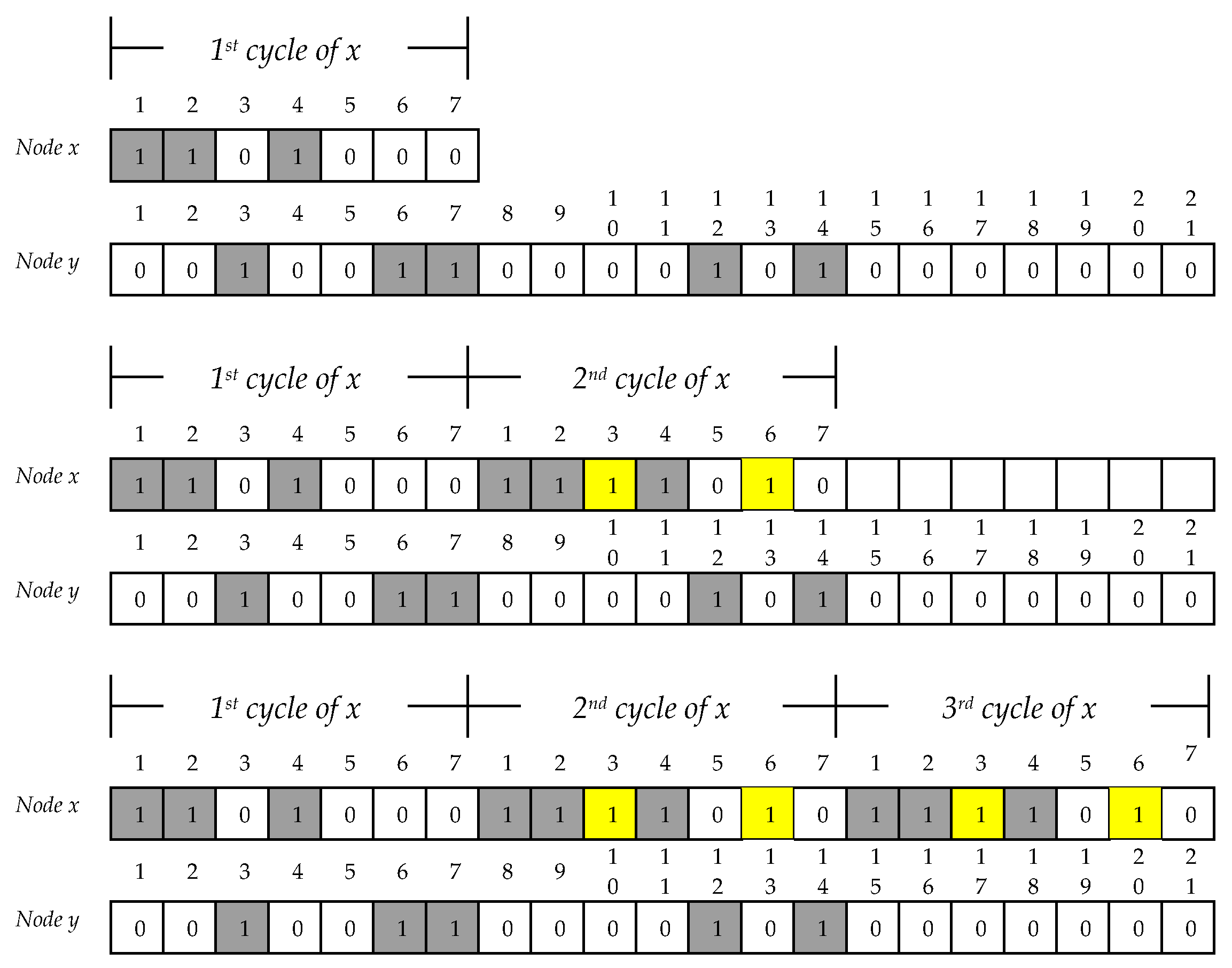
The fundamental idea of solving the asymmetric NDP is to incorporate the original block designs with multiples of k. The asymmetric NDP can be resolved by integrating the concept of multiples of k with the original block designs. The primary concept of the multiples of k is that if a slot number is the same as a multiple of k then the proposed algorithm activates that slot. Thus, the multiples try to cordinate the wake-up time of two nodes operating at different duty cycles and provide the two nodes a chance to locate each other at the same time.

There are two different neighbor discovery schedules: one is a (7,3,1)-design and the other is obtained from a (21,5,1)-design. The duty cycle of these two block designs is not symmetric (asymmetric duty cycle). Hence, two nodes cannot communicate with each other because the two block designs do not have at least one overlapping awakening slot. As seen from Figure 5, there is no common awakening slot between nodes x and y. In Figure 5, node x follows the (7, 3, 1)-design and y utilizes the (21, 5, 1)-design. Therefore, it was possible to apply our proposed asymmetric neighbor discovery algorithm to this problem. Initially, node x may think that there is no neighbor within its communication range in the first round of the duty cycle. There are two options in this situation: First, there is no neighbor in practice. Second, there are neighbors around node x; however, x and its neighbors cannot meet each other because of different duty cycles. We have an opportunity to enable them to talk to each other with the proposed algorithm. From the second cycle, the proposed mechanism can begin to work. In Figure 5, for the first time, x has three awakening slots: 1, 2, and 4. Our asymmetric algorithm starts waking up slot numbers 3 and 6 because these number are multiples of three. From this second cycle, the proposed mechanism turns on its process. Even if node x wasted six awakening slots in the first and second duty cycles, nodes x and y still cannot talk to each other. However, the node following a (21,5,1)-design also thinks that there is no neighbor for communication. 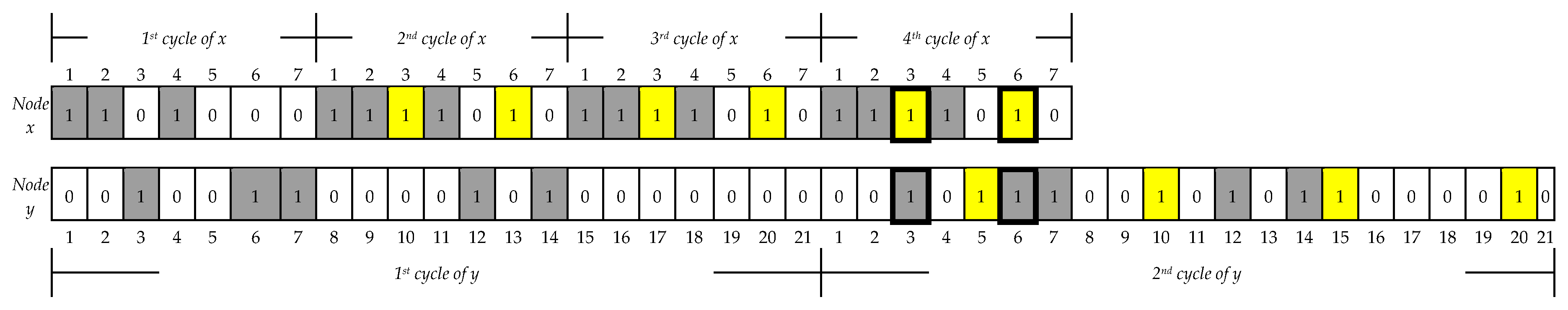Node y proceeds with the proposed mechanism. Figure 6 illustrates that node y wakes up slot numbers 5, 10, 15, 20, which implies that y adopts multiples of five. The yellow color in Figure 5 and Figure 6 represents additional awakening slots that occur using the proposed mechanism. 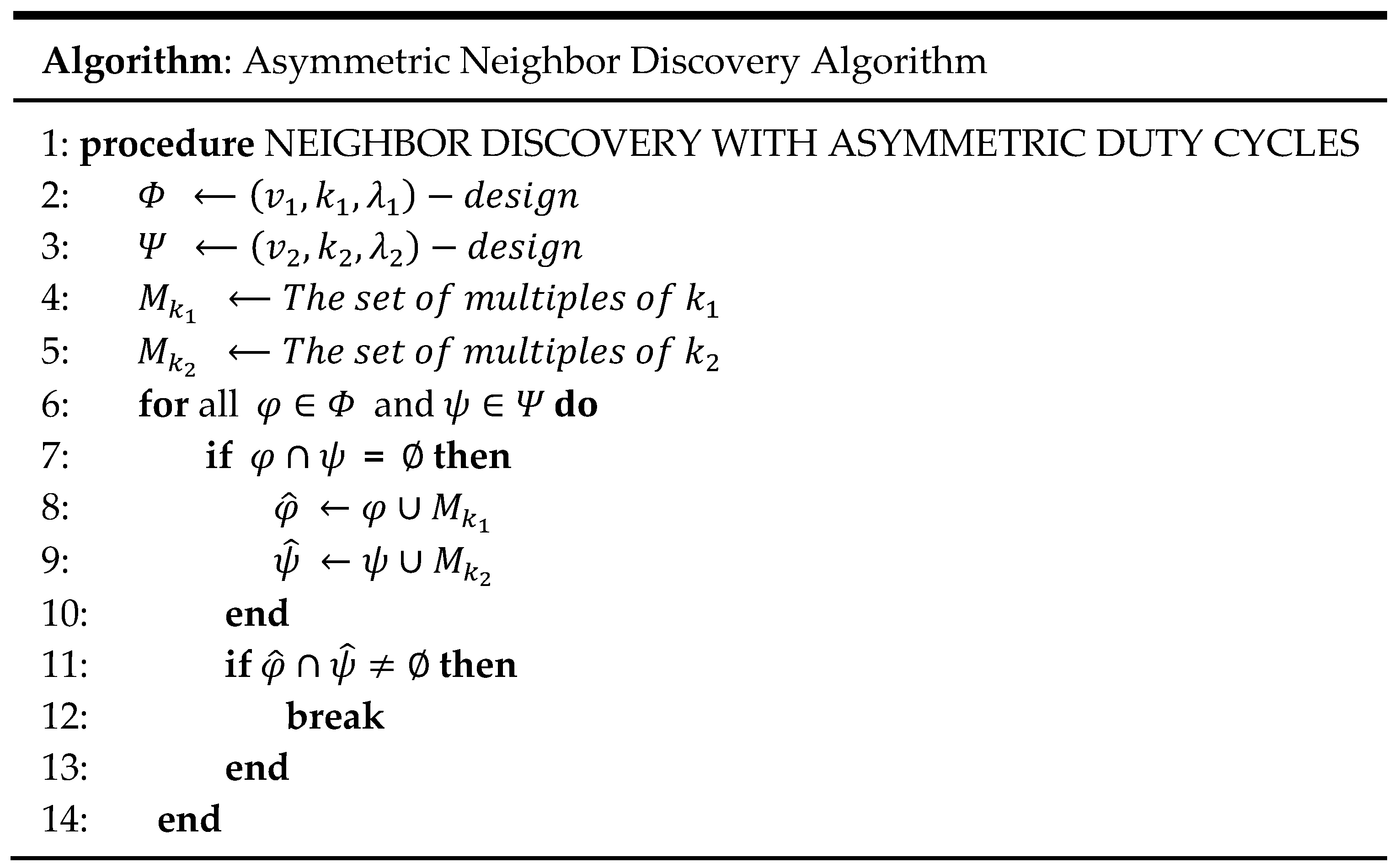Both x and y finally talk to each other twice in the fourth cycle of x and the second cycle of y, respectively, in Figure 6. The proposed asymmetric neighbor discovery algorithm is shown in Figure 7.

7. Numerical Analysis

The study of sensor network protocols [26] shows that the most energy consumption in wireless networked devices occurs during radio communication and idle listening. Idle listening activates a radio interface and waits for the signal from neighboring nodes to maintain network connectivity. If a node wakes up and remains idle, then it wastes energy without any activity. Therefore, the main goal of neighbor discovery optimization is to minimize idle listening time while maintaining network connectivity. Both minimum discovery latency time and a small amount of energy are critical requirements to achieve the primary goal. In Section 7, we present the numerical analysis conducted by comparing and analyzing the performance of certain representative neighbor discovery protocols and ours. There are two performance metrics we considered in numerical analysis: discovery latency time and energy consumption. The first metric is significant because it represents the worst-case neighbor discovery latency. The second one is also crucial because it involves the energy usage of each node.

It is easy to calculate the worst-case discovery latency time once a target duty cycle is provided. There are different duty cycles in an asymmetric case: one is lower than the other. We only considered a lower duty cycle that primarily influences the performance of neighbor discovery in an asymmetric scenario. Unfortunately, the node with the lower cycle cannot discover its neighbors until the total number of slots are utilized in a worst-case scenario. For the numerical study, we first defined the main parameters such as duty cycle, discovery latency time, and the number of active slots for the analysis of discovery latency.

Table 1. Comparison of different discovery protocols.

Protocol	DC	L	Active slots
Disco [12]	$\frac{p_1+p_2}{p_1·p_2}$	$p_1·p_2$	$p_1+p_2$
U-Connect [13]	$\frac{p+1}{p^2}$	p2	$\frac{3p-1}{2}$
Searchlight [15]	$\frac{2}{t}$	$\frac{t^2}{2}$	t
Combinatorial + Multiples of k	$\frac{\left(k+1\right)+\alpha }{k^2+k+1}$	$k^2+k+1$	$\left(k+1\right)+\alpha$

lists three main parameters considered among the representative neighbor discovery protocols and our protocol. The next step was to determine an appropriate parameter for each protocol to apply these parameters to compute the worst-case discovery latency time.

Table 2. Parameter settings for numerical analysis.

Protocol	DC
	10%	5%	2%	1%
Disco	p1 = 13, p2 = 31	p1 = 29, p2 = 61	p1 = 97, p2 = 101	p1 = 191, p2 = 211
U-Connect	p = 11	p = 23	p = 53	p = 101
Searchlight	t = 20	t = 40	t = 100	t = 200
Combinatorial + Multiples of k	k = 9	k = 19	k = 49	k = 97

lists the parameter settings for calculating the discovery latency of each protocol based on 10%, 5%, 2%, and 1% of the duty cycles.

Table 3. Total number of slots of different discovery protocols.

Protocol	DC
	10%	5%	2%	1%
Disco	403	1769	9797	40,301
U-Connect	121	529	2809	10,201
Searchlight	200	800	5000	20,000
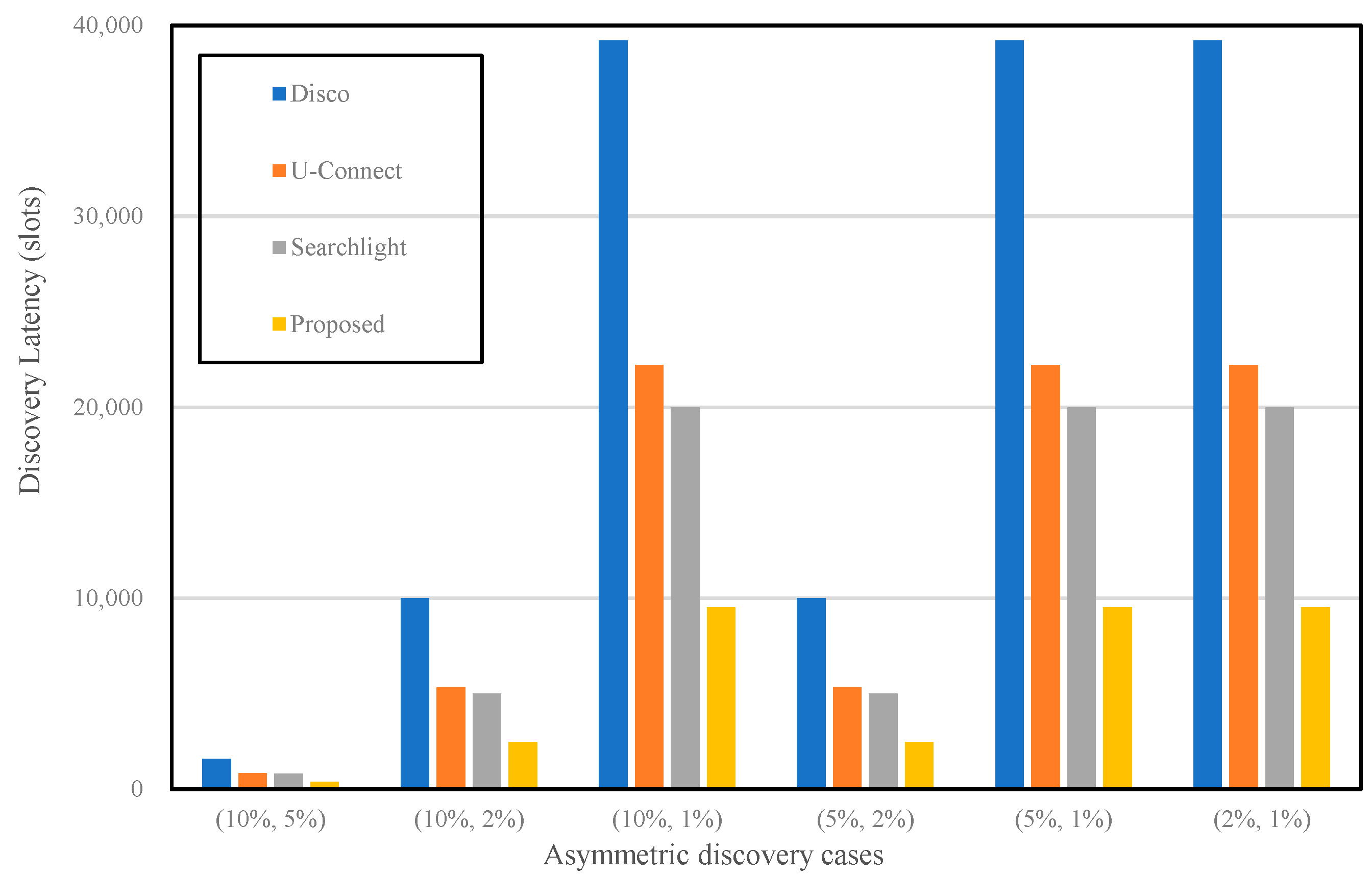
Combinatorial + Multiples of k	91	381	2451	9507

depicts the worst-case discovery latency with respect to the total number of slots. As we can realize from Table 3, the proposed approach has the smallest number of slots when compared to the three neighbor discovery protocols (Disco, U-Connect, Searchlight). It proves that the two nodes adopting the proposed protocol might have a chance to discover their neighbors faster than when utilizing other protocols in an asymmetric situation. Figure 8 shows that the total number of slots is different in several asymmetric scenarios.

It is guaranteed that the number of active slots is closely related to energy consumption of the wireless sensors. When the node is in the active state, it turns its radio on and is ready to transmit and receive packets. Transmitting and receiving packets are some of the most expensive activities. That is why active slots represent energy consumption. From this perspective, the numerical analysis of energy consumption usually computes the number of active slots. Table 1 lists the number of active slots for each neighbor discovery protocol. In the proposed mechanism, the number of awakening slots might be different at given duty cycles; therefore, a variable α is borrowed in Table 1. The variable α can be decided based on the multiples of k. k is not fixed in our proposed algorithm. If k is a small value, then the number of active slots will be increased. Otherwise, the active slots will be decreased. For example, if the duty cycle is 10% and k value is 9, the variable α will be approximately 10.

The following scenario was considered for the analysis of energy consumption: one node has a higher duty cycle than the other. This node cannot discover its neighbor within the first round of its duty cycle. For instance, node A uses 10% of the duty cycle (higher duty cycle) and the other node B uses 5% of the duty cycle (lower duty cycle). A cannot talk to B within the first round of its duty cycle. The next step is to compute the total number of active slots among the four neighbor discovery protocols. 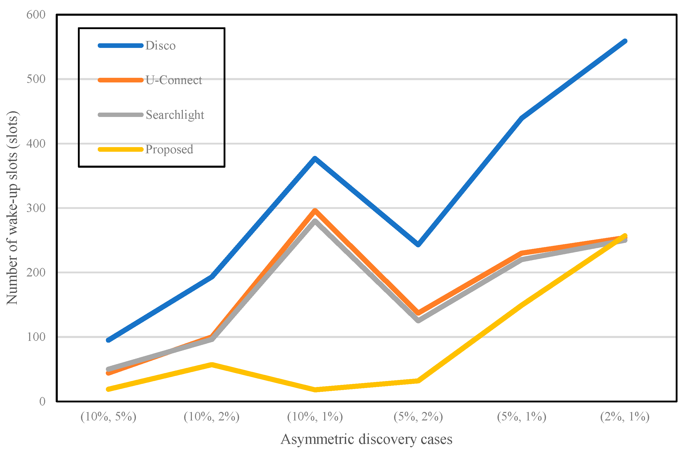Figure 9 shows the total number of active slots for the four different algorithms. In general, 1% of the duty cycle requires a bigger number of active slots than others. Disco, U-Connect, and Searchlight show a similar pattern. For example, the primary concept of Disco and U-Connect use a prime number to activate the node. They make each slot active according to the multiples of a given prime number. If the given prime number is getting bigger, similar to 1% of the duty cycle, the offset between one active slot and the other is also increased. Therefore, the asymmetric case of (10%, 1%) has a larger value than the cases of (10%, 5%) and (10%, 2%) in Figure 9. However, the proposed algorithm represents a different shape when compared to other protocols because the waking-up pattern is asymmetrical. In general, the total number of active slots in the proposed technique is the lowest when compared to that of other protocols. The discovery latency in Figure 8 and the number of awakening slots in Figure 9 illustrate a reverse trend from (10%, 1%) to (5%, 2%). This situation happens because it is based on the selection of variable α. A simulation or real experiment with mobile sensors will be required to verify that our numerical study is reasonable. Consequently, our method can discover neighbors much faster than others with minimum energy consumption.

8. Conclusions

We analyzed neighbor discovery optimization for low-power, low-cost communication networks in this paper. As we stated in the introduction section, these networks consist of various heterogeneous communication devices. Every time the network participants are required to communicate with their neighbors, they should first comprehend that there are existing neighbor nodes in their communication range. After locating their neighbors, they try to connect with them and finally establish a network connection. The communication mechanism we considered in this paper focused on M2M communication in a distributed manner. This communication is mostly similar to the communication method of WSNs.

In this paper, we developed an asynchronous and asymmetric neighbor discovery protocol by combining the traditional block designs and the multiples of k. The shortcoming of the block design is that it might be possible to use it only for certain duty cycles. We recommended a block construction scheme by combining two block designs to support any desired duty cycle. Furthermore, the traditional block design can assist only symmetric duty cycles and not asymmetric cases. We provided an asymmetric neighbor discovery algorithm by introducing the use of the multiples of k to overcome the weakness of typical block designs.

We performed a numerical study by analyzing the performance of existing representative neighbor discovery protocols and comparing our proposed algorithm with other protocols. The numerical analysis revealed that the proposed algorithm utilizes the minimum number of active slots, which implies that our protocol discovers neighbors faster and wastes less energy than other protocols.

Future research directions should attempt a simulation study or a real experiment on distributed network environment settings. This study can verify that the total number of slots is related to the energy consumption and network lifetime of nodes in the network. In addition, selecting the parameter values using the concept of multiples might affect the performance of the neighbor discovery protocol that we proposed with a variety of parameter settings.

In addition, one of the significant research directions of neighbor discovery is the IP version 6 (IPv6) NDD [27]. In WSN environments, there is no concept of IP address in each wireless sensor. In the future, IoT devices could be either IP address or ad hoc based. Therefore, we plan to focus on a neighbor discovery study in IPv6-based mobile devices.