Article

Research on a Tool Wear Monitoring Algorithm Based on Residual Dense Network

Key Laboratory of Advanced Manufacturing Technology, Ministry of Education, Guizhou University, Guiyang 550025, China
*
Author to whom correspondence should be addressed.
Symmetry 2019, 11(6), 809; https://doi.org/10.3390/sym11060809
Submission received: 21 May 2019 / Revised: 12 June 2019 / Accepted: 16 June 2019 / Published: 19 June 2019
(This article belongs to the Special Issue Novel Machine Learning Approaches for Intelligent Big Data 2019)

Abstract

:
To accurately and efficiently detect tool wear values during production and processing activities, a new online detection model is proposed called the Residual Dense Network (RDN). The model is created with two main steps: Firstly, the time-domain signals for a cutting tool are obtained (e.g., using acceleration sensors); these signals are processed to denoise and segmented to provide a larger number of uniform samples. This processing helps to improve the robustness of the model. Secondly, a new deep convolutional neural network is proposed to extract features adaptively, by combining the idea of a recursive residual network and a dense network. Notably, this method is specifically tailored to the tool wear value detection problem. In this way, the limitations of traditional manual feature extraction steps can be avoided. The experimental results demonstrate that the proposed method is promising in terms of detection accuracy and speed; it provides a new way to detect tool wear values in practical industrial scenarios.

1. Introduction

Manufacturing is a critical part of a national economy. With economic globalization and the emergence of Industry 4.0, it has become increasingly important to enhance efficiency and promote business transformation of enterprises. Research in the area of prognostics and health management (PHM) plays a pivotal role in promoting the transformation of the production industry [1]. Current topics of interest in the PHM focus on identifying potential relationships within the data by searching and analyzing massive amounts of industrial data with the aid of artificial intelligence algorithms. The goal of such research is to further optimize production processes; recent results have allowed the maintenance of industrial equipment to evolve from expert, experience based methods to automated adaptive learning methods. Ultimately, these intelligent detection methods can help to improve the efficiency of manufacturing processes from a number of perspectives.
Tool wear monitoring is an important aspect in the PHM area. During the machining process, the tool wear occurs, which affects the quality of the machined surface and may lead to the risk of the machine tool damage [2]. Tool wear measuring methods can be categorized into direct and indirect methods. For the direct methods, the tool wear value can be obtained directly by a machine vision, surface measurement, or laser technique. However, it is often necessary to interrupt the manufacturing process due to the influences of interference sources such as coolant. This results in a detrimental impact on productivity in real-time environments, which limits their practicability [3]. For the indirect methods, sensing equipment is used to collect the signals and acquire the signal features related to the wear value. Since the sensor does not have direct contact with the tool and does not affect the machining process, this class of methods is well-suited for practical working conditions in production workshops. At present, sensor-based tool data acquisition mainly includes the following signals; cutting force, vibration, acoustic emission, current, and torque [4,5,6]. In traditional tool wear detection methods, the acquired data is preprocessed with normalizing and denoising methods. Then, design features are manually extracted from the time domain, the frequency domain, the time-frequency domain, respectively, to reduce the dimensionality. Finally, a hidden Markov model (HMM), neural networks, or support vector machine (SVM) is used for the classification or regression purposes [7,8,9,10,11,12].
Most of the current tool wear detection algorithms collect signals with the indirect methods, which is implemented using machine learning algorithms. For example, Liao et al. propose a tool wear condition monitoring system based on the acoustic emission technology [7]. By analyzing representative acoustic signals, the energy ratios from six different frequency bands are selected from the time-frequency domain. These are used as a classification feature to determine the amount of tool wear. In this method, the SVM is used as the classification method, which can ultimately achieve the accuracy ratio of 93.3%. In [10], the cutting force signal and the multiscale hybrid HMM are combined to monitor the wear state of the tool. From the perspectives of local and global analyses, this method can deeply capture the tool wear state information; accurate performance monitoring of the tool wear value is achieved. The experimental results indicate the hybrid approach achieves better performance in comparison to that obtained by the use of the HMM alone. Zhang et al. apply the multifractal theory to calculate the generalized fractal dimensionality of the acoustic emission signal during the cutting process [12]. Here, the generalized dimensional spectrum of the acoustic emission signal is obtained under different tool conditions. The generalized fractal dimensionality and cutting process parameters are used as the input feature vector of a backpropagation neural network (BPNN), where the initial weight value of the network is optimized with a genetic algorithm. The experimental results show that this method is able to predict the tool wear effectively, where the tool machining efficiency can be further improved. The above methods are often constrained by the quality of the extracted features; manually refining the features requires researchers to master specific experience and skills related to the production environment. Therefore, the enhancement of the machine learning models remains rather limited.
In recent years, rapid developments have seen for deep learning methods based on artificial neural networks. These methods can extract different features by building a deep neural network structure. In contrast, the traditional methods are only able to extract specific features. Multifeature learning can describe the research problem more comprehensively and improve the accuracy and robustness of the algorithm. Therefore, deep learning methods have demonstrated superior performance in various classification and regression tasks; in particular, they have received attention in the fields of image and speech processing [13,14,15]. Remarkably, the deep neural network can replace the feature extractor and classifier (regressor) in conventional feature learning theory. It can be considered as an end-to-end model, which does not depend on the complicated preprocessing of original data. As a result, these networks are more concise and fast. The deep learning method has shown promising results in related areas of the PHM, and has been applied to fault diagnosis, equipment life prediction, and tool wear detection [16,17,18,19]. In [16] a bearing fault diagnosis method is proposed based on a fully connected competitive self-encoder. This model can explicitly activate certain neurons from all of the samples of a minibatch, where the life cycle sparsity can be encoded into the features. A soft voting method is further used to make predictions on the signal segments generated from the sliding window. The experimental results show that the methods using a two-layer network can obtain higher diagnostic accuracy under normal conditions and can also demonstrate better robustness than methods with deeper and more complicated network models. Zhang et al. propose a transferring learning and Long Short-Term Memory (LSTM) based model for predicting the remaining life of equipment [18]. This research addresses the problem of a small sample size, due to the difficulty in acquiring the faulty data. In particular, this model can be pretrained on different, but related, datasets. Subsequently, the network structure and the training parameters are finely tuned for the target dataset. The experimental results demonstrate that the transfer learning method is capable of improving the model’s prediction accuracy using a small number of samples. Zhang et al. apply the wavelet packet transform method to transform the acquired tool vibration signal to the energy spectrum, which is further used as input into the convolutional neural network (CNN) [19]. Therefore, features can be automatically learnt and accurately classified with the powerful image feature extraction capability of the CNN. It is indicated in [19] that a deep learning based CNN can achieve superior accuracy in comparison to other classical tool wear prediction models for the milling cutter wear classification problem.
In summary, significant progress on deep learning methods has been reported in a variety of areas. However, research on their use in tool wear monitoring is just beginning to emerge. The end-to-end processing the deep learning methods provide has the potential for significant impact in manufacturing industries. A crucial, open research area is the development of algorithms that are capable of adaptively extracting features from time-domain signals and can also strike a balance between accuracy and speed by adjusting the training methodology and model structure.

2. The Detection Method of Tool Wear Value

2.1. Signal Preprocessing

In this paper, acceleration sensors are used to collect the three-axis vibration signal generated by the cutting tool; these signals are used for the tool wear value detection. Acceleration sensors are simple to measure and are convenient to install and monitor. Since the vibration signal directly comes from the cutting work area, the sensitivity is relatively high and the response time is fast. However, the collected real data suffer from unequal length, redundancy, and high noise. Therefore, it is necessary to perform denoising and uniform scaling on the collected signals.
Random noise will inevitably arise in workshop production environment and equipment interference. So noise often exists in the production process, especially during precision machining. These noises are usually regarded as Gauss noise in signal preprocessing. The feature extraction and wear value detection algorithms are affected by the noise. To reduce the influence of noise on the detection results, the wavelet threshold denoising method is applied to the originally collected signal. In Figure 1, a flow chart of the wavelet threshold denoising method is presented.
The selection of wavelet mother function and threshold determines the performance of wavelet threshold denoising method. Daubechies and Symlets wavelet mother functions are often used to denoise vibration signals in engineering; the soft or hard thresholding methods are often used in threshold processing. The wavelet coefficients obtained by the hard threshold method are not continuous at the threshold, which may cause oscillation when reconstructing the signal. But the wavelet coefficients obtained by soft threshold method have good continuity and the processed signals are smooth. Its expression can be represented as follows
W ^ j , k = [ sign ( W j , k ) ( | W j , k | λ ) | W j , k | λ 0 | W j , k | λ
where j is the scale of wavelet decomposition; k denotes an index sequence of wavelet coefficients; W j , k and W ^ j , k are original wavelet coefficients and the wavelet coefficients processed by soft threshold, respectively; λ represents the threshold; and the heuristic threshold method is used to determine it. More specifically, Daubechies and Symlets wavelet mother functions are used with the decomposition scale of three levels. Since most of the effective vibration signals generated during tool processing are concentrated in the low-frequency part, the threshold for the high-frequency signal processing is chosen as follows; the first layer of the high-frequency is set to zero and the soft thresholding method is used for the second and third layers. The SNR of different wavelet groups are shown in Figure 2.
In Figure 2, the denoising performance of db18 wavelet mother function is the best, and its effects are shown in Figure 3. It can be seen that the original vibration signal becomes relatively smooth after applying the wavelet threshold denoising method. In addition, the form of the original signal is restored to a great extent.
After the signal denoising, the sample size must be reduced and unified to satisfy the speed and sample size detection requirements. In this paper, the vibration signal generated by each tool feed is segmented into multiple time-domain signals, where each has a length of 5000 points to reduce the computational complexity during network training. These samples are independent and nonoverlapping with each other. In the meantime, it would be beneficial to the robustness of the network and reduce the overfitting issue due to the increased sample size. The processing steps are as follows; choose 50,000 consecutive points in the middle of the signal and segment the signal into 10 samples with lengths of 5000. These 10 samples correspond to the same label of the tool wear value.

2.2. Residual Network

The residual network (ResNet) proposal by Kaiming He et al. in 2015 has effectively resolved the gradient explosion and network divergence problems due to the increase in the number of layers in the deep CNN [20]. ResNet has profoundly affected research in deep learning networks as it allows the number of network layers to be further increased, and deeper features can be extracted as a result. The basic component of the ResNet is the residual block, which is illustrated in Figure 4.
In the figure, the input signal is defined as x. The feature extraction layer is defined as Conv, where a CNN is generally used. The degree of feature extraction reflects the cognitive and learning ability of the model, which is the basis of classification and regression tasks in deep learning and machine learning. The residual is defined as F(x), i.e., the difference between the feature H(x) learned from the convolutional layer and the original input signal (or the output from the previous layer). The relu is the activation function. There are different variations of the relu function, such as LReLU, PReLU, CReLU, ELU, and SELU. The main difference of these variations is how these functions map the negative value of the features. It should be noted that the relu function can avoid the gradient disappearance issue during the training process and can speed up the training process. Let the output signal obtained by the residual block be y, and its expression can be represented as follows
y = F ( x , { W i } ) + W s x
where x is the input signal, W i denotes the parameters of the convolution layer, F ( x , { W i } ) represents the output feature from the convolutional layer, and W s represents a nonlinear transformation to transform the dimensionality of x to the same dimensionality of the feature F for the convenience of their addition.
In the original residual network, the residual is calculated from the local residual block; the input of the residual block is the output of the previous layer. As the network becomes deeper, the error accumulates and the local residual error increases accordingly. Tai et al. propose a recursive learning method to improve the residual network for the application of super-resolution image reconstruction [21]. The method is called the Deep Recursive Residual Network (DRRN). The main idea of DRRN is to make full use of both global residuals and local residuals. In particular, each residual unit shares the same input, i.e., the output from the first convolutional layer of the recursive block. Within a recursive block, the corresponding parameters of the convolutional layer in each residual unit are shared. The structure of the basic recursive residual block is illustrated in Figure 5.
The DRRN adjusts the existing ResNet structure based on the image super-resolution reconstruction method by incorporating the global residual and adopting a deeper network structure. In this way, further improvements have been demonstrated in the experimental results.

2.3. Tool Wear Detection Method

2.3.1. Network Structure

Motivated by the work in DRRN, a new tool wear detection method is proposed by using the DRRN idea, where further improvements on the recursive residual block of the DRRN are made. The DRRN is originally used to process two-dimensional images. However, the signal in this paper is a one-dimensional signal, and the number of data samples is small. Therefore, improvements and simplifications are needed to tailor the model for the tool wear detection problem. The DRRN network is further improved in this paper in two ways. First, local residuals and global residuals are comprehensively incorporated. Second, the dense network (DenseNet) structure is considered in building up the model [22]. These improvements alleviate the gradient disappearance problem, enhance feature propagation, support the possible of reuse features, and reduce the number of parameters. It should be noted that the original dense network does not contain the residual information. The main contribution of this paper is to incorporate the residual structure, and connect features in series. Before the data are passed to the next layer, they are normalized using the batch normalization (BN) method to transform the mean to be zero and the variance to be one [23]. The key point is to add learnable parameters γ and β for reconstruction, where the formula can be given as follows
y ( k ) = γ ( k ) x ^ ( k ) + β ( k )
where k is the index value of layers and x ^ represents the standardized feature element, when γ ( k ) = V a r [ x ( k ) ] and β ( k ) = E [ x ( k ) ] it can restore the distribution of the features that the original network is supposed to learn and avoid changes in the original features distribution caused by the BN process. The BN algorithm flow is as follows
(1)
Calculating the mean value of all features
μ B = 1 m i = 1 m x i
where m is the size of a minibatch and x i is the i-th value in a feature.
(2)
Calculating the variance of all features
σ B 2 = 1 m i = 1 m ( x i μ B ) 2
(3)
Normalization
x ^ i = x i μ B ε + σ B 2
(4)
Reconstructing the feature
y i = γ x ^ i + β B N γ , β ( x i )
In particular, BN can make the parameters of each layer similar within the numerical interval. Therefore, the deep network training process can become more stable, and the gradient explosion problem can be avoided. In this paper, the designed dense unit is shown in Figure 6.
In this figure, the input signal is represented by x, and the output signal is represented by y. After the 1D convolution kernel of size = 5 and 3, the local residual F1(x) and the global residual F2(x) are calculated, and the local feature H1 and the global feature H can be subsequently obtained as follows
H 1 = F ( x , { W 3 } ) + W s x
H = F ( H 1 , { W 5 } ) + W s x
where H1 represents the local feature from the third convolutional layer as shown in Figure 4, and H represents the global feature from the fifth convolutional layer.
By using the idea of the dense network, the local feature can be combined in series with the global feature to obtain the output signal y, which can be expressed as
y = W s [ H 1 , H ]
where W s represents a nonlinear transformation to make the dimensionality of the output features to be the same. The operation in (9) represents that the output of the dense block is the combined output from all of the previous residual features.
According to the idea of the dense network, a transition layer is added after a dense block. In this paper, the transition layer is composed of a 1D convolution layer with a kernel size = 1, a pooling layer, and a dropout layer. An average pooling approach is adopted by the pooling layer. The purpose of the transition layer is to reduce the dimension of the input features provided to the next layer, and ensure the number of features provided to the dense block remains the same each time. The amount of computation can be reduced by a downsampling approach with pooling. The purpose of adopting the Dropout layer is to randomly reduce the number of neurons and prevent overfitting. The proposed network structure in this paper exploits the ideas of the residual network and the dense network; it is named the Residual Dense Network (RDN). The structure diagram of the RDN network is shown in Figure 7.
As shown in the figure, the RDN network is composed of three residual dense blocks, two transition layers, one convolutional layer, one pooled layer, and one fully connected layer. A convolution kernel of size = 13 is used in the first convolution to expand the receptive range and capture the global features of the signal better. The dense block can then identify subtle features around each signal point by using convolution kernels of size = 5 and size = 3. The parameters on each layer of the network are set as shown in Table 1.

2.3.2. Network Training

After setting up the network structure, the dataset needs to be divided into training and validation sets. The vibration data and corresponding labels of wear values are collected from four tools in the experiment. In particular, the data from three tools is divided into training sets, and the data from the remaining tool is used as a validation set. The training set is input into the network for training. The validation set is used to test the network performance, determine whether the network is overfitting, and calculate the network performance index. The output value in the network is the predicted tool wear value, and the network type is a regression network. The mean square error is used as the loss function, which can be calculated as follows
J M S E = 1 n i = 1 n ( x i x i ) 2
where n is the number of training samples and x i represents the true value of the wear of the ith sample. The maximum value of the flank wear after milling is used as the real label and x i is the predicted value of the wear of the ith sample.
Since the weights are shared for each layer of the CNN, W l represents the shared weight in the lth layer, and b l is the offset of the lth layer. Subsequently, the output of the lth layer can be expressed as
y l = f ( W l x l 1 + b l )
where f ( ) represents the relu activation function.
The gradient descent method is used to back propagate the updated weights and offsets until the loss function is less than the expected value. The parameter updating formula of the weight and offset can be expressed as
W = W η J M S E W
b = b η J M S E b
where η is the learning rate with η ( 0 , 1 ) . Note that the learning rate affects the convergence speed of the loss function. A smaller learning rate leads to a slower convergence speed. If the learning rate is too large, the loss function does not converge. In this paper, the initial learning rate is 0.001.

3. Experimental Results and Analysis

The intelligent manufacturing laboratory of Guizhou University, Guizhou Province, China, is selected as the validation platform. The experimental equipment is as follows; one computer numerical control (CNC) milling machine for machining workpieces; one die steel (S163H) as the workpiece to be machined—the machining tool has a cemented carbide 4-edge milling cutter (diameter of 6 mm) and its surface is covered with layers of titanium aluminium nitride coating; and a signal processing unit. The cutting parameters are set as shown in Table 2.
The signal preprocessing mainly transmits the three-axis vibration signal from the tool processing to the upper computer through the acquisition unit. The upper computer performs the wavelet threshold noise reduction. In traditional machine learning methods, the corresponding features are first extracted from the time domain, the frequency domain, and the time-frequency domain. Then, these methods are used to reduce the dimensions of the features and input them into the neural network (or SVR regression) in order to obtain the wear detection value. In this paper, the deep RDN model is used to adaptively extract features from the time-domain signal after the noise reduction, and the wear detection value is obtained. The network training parameters are as follows; the learning rate is initialized to 0.001 and set to exponential decay, the batch size is 32, the epoch is 100, the optimizer uses Adam, the weights and bias are randomly initialized.

3.1. Signal Processing Unit

The signal processing unit can be divided into a data acquisition unit and an upper computer analysis unit. The data acquisition unit consists of an acceleration sensor, a constant current adapter, a digital acquisition card, an acquisition software program, and a microscope (workflow as shown in Figure 8). Before the start of the data acquisition, three accelerometers are installed in the X, Y, and Z directions of the workbench. Then the magnification of the microscope is adjusted and the measurement calibration of the microscope is completed. The sampling frequency of the digital acquisition card is set to 20 KHz. Each tool performs 330 feeds in the X-axis direction, with a feed of 200 mm each time. When the machining completes, the cutter is removed from the machine and a picture is taken. The measurement process selects the position of the rear edge as the measurement position. This position is the most prone to wear. The same datum line is used to ensure the position remains unchanged during the measurement. The wear value is calculated by subtracting the length of the current rear edge from the last rear edge length.
The hardware configuration of the upper computer analysis unit is as follows; Intel Core i7 7700 K processor, clocked at 4.2 GHz; 32 GB memory; and two linked GeForce 1080 Ti graphics cards. The software uses the Ubuntu 16.04 as the operating system; the deep learning framework uses Keras as the front-end and TensorFlow as the back-end. Before the model is trained, the vibration signal generated by each tool feed is segmented into 10 time-domain signal samples of length 5000. After that, the samples from three tools are scrambled as the training set; the samples from the remaining tool are used as the validation set.

3.2. Evaluation Indicators

In this paper, the root mean square error (RMSE), the coefficient of determination R-square, and the mean absolute percentage error (MAPE) are used as the evaluation indicators of the prediction accuracy. Specifically, the RMSE indicates the degree to which the predicted value deviates from the true label. The closer the value is to zero, the better the performance is. The RMSE calculation is as follows
RMSE = 1 n i = 1 n ( Y i Y i ) 2
where Y i is the true label value of the ith sample wear value, here it represents the tool wear value measured by the microscope; Y i is the predicted value of the ith sample wear value, here it represents the predicted value of designed model; and n is the total sample number of the test set, here it represents the number of vibration samples for prediction.
The coefficient of determination R-square represents the degree of fit between the predicted value of the tool wear value and the real label. The closer the value is to one, the better the fit is. The R-square calculation is as follows
R 2 = 1 i = 1 n ( Y i Y i ) 2 i = 1 n ( Y i Y i ) 2
where, Y i represents the mean value of all the true label values in the test set Y i = 1 n i = 1 n Y i .
The MAPE represents the mean value of the absolute value of the relative error. The closer the value is to zero, the better the prediction performance is. The MAPE calculation is as follows
MAPE = 1 n i = 1 n | Y i Y i Y i | × 100 %

3.3. Experimental Results of Network Structure Comparison

3.3.1. Impact of BN and Dropout Strategies on Model Performance

In the experiment, we mainly focus on the impact of the BN batch normalization and the Dropout regularization strategy on the network convergence performance in RDN. The network convergence performance is compared on the training set and the validation set as the basis for judging the results. The comparisons are performed by (1) removing the BN layer of the RDN network and (2) removing the Dropout layer of the RDN network. The comparison results are shown in Figure 9.
According to the results in the figure, there is no gradient explosion or dispersion in the three network structures, and the network convergence speed is fast without overfitting. It indicates that the RDN convergence performance is superior and the generalization ability is strong. The RDN network with the BN and Dropout layers converges faster than the RDN network with the BN layer removed or the Dropout layer removed. After 15 iterations, the loss function value is close to its lowest value. In the subsequent iterative process, changes of the loss function values are small and the convergence performance is good. However, the performance of the RDN network with the BN layer removed or the dropout layer removed is impeded. The model needs to iterate 35 times in the training set to converge to the minimum value, the convergence speed is slower on the verification set, and the obtained loss function is also higher. The above experiments demonstrate the effectiveness of the RDN model proposed in this paper, which adopts the BN block and the Dropout layer.

3.3.2. Impact of Network Layer Number on Model Performance

In order to verify the impact of different network depths on the performance of the model, 24-, 44-(the network used in this paper), and 84-layer networks have been selected for analysis. All of the networks use the same dense block and transition block. The difference is in the inconsistent number of dense blocks. The comparison of the convergence performance on the training set and the validation set for the varying depths is shown in Figure 10.
It can be shown that a certain depth of the network can better extract the effective features and reduce the RMSE between the predicted value and the true value. However, when the network structure is continuously deepened to a certain extent, gradient dispersion occurs in the model. This causes the loss function to remain at a certain large value; it cannot be decreased. During the training progression, the network model with a depth of 44 layers has the best convergence performance. The mean value of the loss function dropped to 3.82 in the last five iterations on the training set, and reached 94.67 on the validation set. Therefore, a more appropriate network depth can improve the feature extraction quality and cause the loss function value to continually decrease. At the same time, the choice of depth balances the network complexity and prediction accuracy, reduces the hardware requirements of the network, and makes it more portable and scalable.

3.4. Comparison Results of Deep Learning Models

The regression performance of the RDN method proposed in this paper is shown in Figure 11. The true wear value in the figure is measured by microscope after each feed. In the figure, the RDN has a large prediction error value at the initial wear stage and at the severe wear stage; the predicted value is relatively stable in the moderate wear stage. This aligns with the actual need for tool wear detection. The results also show the RDN learns the data features adaptively to achieve better prediction results, i.e., separate steps to extract and refine features are not needed.
In the deep learning model, CNNs and cyclic neural networks are commonly used to deal with sequence problems, such as speech recognition and natural language processing. VGGNet-16 [24] and ResNet-50 are used in the experiment, which have achieved excellent results in the ImageNet competition. In addition, the convolution method is replaced with a one-dimensional convolution. At the same time, the RNN [25] and LSTM [26] models are also selected. The network structure is set to a two-layer structure with neurons of 120 and 50, and then regression is performed after the fully connected layers. The above four models are compared with the RDN proposed in this paper. The results are shown in Figure 12, Figure 13 and Table 3.
The results are the performance of the models on the validation set. It can be seen from the analysis that when the RNN and LSTM models (with certain advantages in processing time series data) are directly used to predict the wear value, their performance is not satisfactory. One reason may be that the above models did not extract the characteristics of the vibration signals well. In addition, the performance may also be due to the model structure and preprocessing method selected in the experiment. For CNNs, VGG-16 has the worst performance among three convolutional structures because the number of convolutional layers is not large; high-dimensional signal features are not extracted. However, the performance results of VGG-16 are better than the designed cyclic neural network. Both ResNet-50 and RDN have achieved satisfactory results. The results show that it is feasible to use CNNs for tool wear value regression.

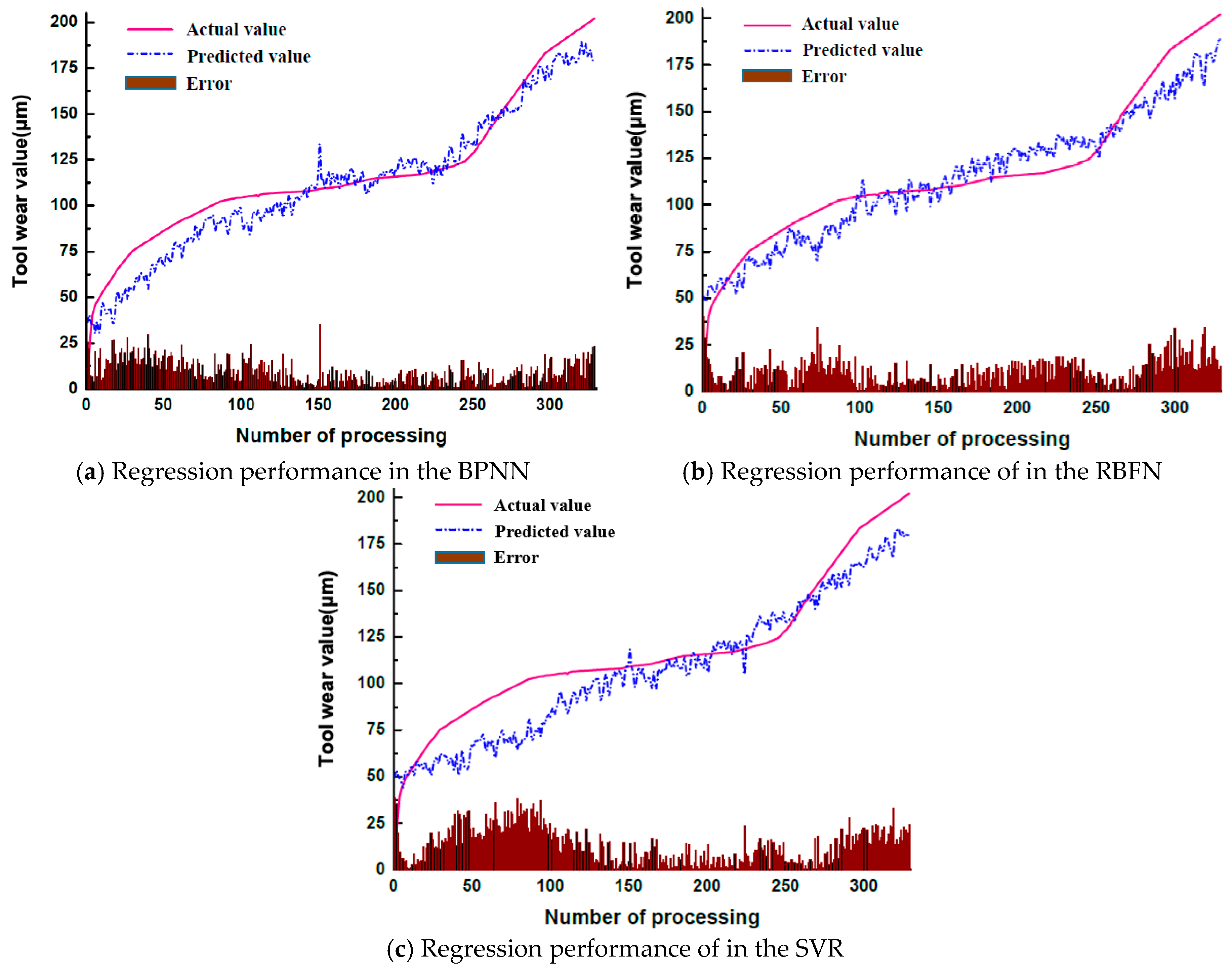
3.5. Comparison Results of Machine Learning Models

In order to further validate the feasibility of the proposed RDN model, a comparative experiment is designed with alternative machine learning models. More specifically, the commonly used models in the traditional tool wear value detection approaches including the BP neural network (BPNN), the radial basis functions neural network (RBFN), and the support vector regression model (SVR) are compared with the RDN network proposed in this paper. The data preprocessing and feature extraction methods are as follows.
(1)
The wavelet threshold denoising method is employed to perform the noise reduction processing on the acquired three-axis acceleration signal.
(2)
The data features of time domain, frequency domain, and time-frequency domain are extracted, and the specific extraction methods are shown in Table 4.
(3)
Pearson’s Correlation Coefficient (PCC) is used to reflect the correlation between the feature and the wear value, and the feature with a correlation coefficient greater than 0.9 is selected as the extraction object to reduce the feature dimension.
(4)
The extracted features are used as the inputs of the machine learning model.
The results are shown in Figure 14, Figure 15 and Table 5.
According to the results, it can be seen that the results obtained from the machine learning models are not stable. Compared to the deep learning model, only the BPNN can achieve better results than the RNN model. This is due to the fact that the accuracy of the network prediction is largely influenced by the data preprocessing, feature extraction, and model structure selection. Deep learning can achieve very strong results with an adaptive feature learning process and a reasonable network depth design. These results can be achieved under the premise of little or no data preprocessing. Compared with the other algorithm models, RDN achieves a significant performance improvement. The time for the forward operation of the RDN is approximately 112 ms. Although this result is not as good as the partial comparison model, the RDN model provides a better balance between time and accuracy. Therefore, it can be adopted to meet the real-time and accuracy requirements in industrial production.

4. Conclusions

In this paper, we propose to innovatively apply the idea of the DRRN, originally used for super-resolution image reconstruction, to the tool wear value detection problem. To be more suitable for this application, the network parameters and the structure are optimized based on the characteristics of the vibration signal, and the loss function is redesigned. In the preprocessing stage, a wavelet denoising procedure is used on the time domain signal of the acceleration sensor, and the redundant signals generated by each tool are segmented into multiple training samples to filter out noise and improve the robustness of the algorithm. Moreover, the DRRN is further improved. Specifically, the global residual, local residual, and dense network ideas are integrated together. A meta-structure, called the RDN, is proposed. To further alleviate the problem of gradient dispersion, BN layers and Dropout layers are added to the network; these have effectively improved the convergence of the network. The feasibility of this method is validated with the milling cutter wear value detection platform. In this experiment, the signal acquisition unit and the upper computer analysis unit are built; the proposed deep learning framework is used to predict the tool wear value. The experimental results demonstrate that the proposed tool wear value detection method is both efficient and accurate, has a clear workflow, and can adapt to the hardware system of most production environments. These results are promising, and indicate the RDN has the potential to meet the stringent requirements of real-time production environments.
In practical production, the working procedures and site conditions are often complicated and variable. The proposed signal acquisition method and prediction model are restricted by the training data volume and processing method, which may not be applicable to arbitrary working conditions. In the future research, the following two directions are worthy of further investigation. First, from the signal acquisition perspective, the generalization capability of the prediction model can be improved by using multiple sensors to monitor the processing. The RDN approach can be extended to combine multisource data fusion technology with deep learning theory. Second, from the perspective of network design, the network prediction performance can be further improved by combining CNNs with other intelligent models.

Author Contributions

Project Administration, Y.L.; Validation, Y.L.; Resources, H.H. and Q.X.; Investigation, Q.C.

Funding

This study was supported by the major project of the National Natural Science Foundation of China (No. 51865004) and the Science and Technology Project of Guizhou Province (No. [2018]5781 and No. [2017]0034).

Conflicts of Interest

The authors declare no conflict of interest. The founding sponsors had no role in the design of the study; in the collection, analysis, or interpretation of data; in the writing of the manuscript, and in the decision to publish the results.

References

  1. Yu, P. A review: Prognostics and health management. J. Electron. Meas. Instrum. 2010, 24, 1007–1015. [Google Scholar]
  2. Zhou, Y.; Xue, W. Review of tool condition monitoring methods in milling processes. Int. J. Adv. Manuf. Technol. 2018, 96, 2509–2523. [Google Scholar] [CrossRef]
  3. Dutta, S.; Pal, S.K.; Mukhopadhyay, S.; Sen, R. Application of digital image processing in tool condition monitoring: A review. CIRP J. Manuf. Sci. Technol. 2013, 6, 212–232. [Google Scholar] [CrossRef]
  4. Patra, K.; Jha, A.K.; Szalay, T.; Ranjan, J.; Monostori, L. Artificial neural network based tool condition monitoring in micro mechanical peck drilling using thrust force signals. Precis. Eng. 2017, 48, 279–291. [Google Scholar] [CrossRef]
  5. Martins, C.H.; Aguiar, P.R.; Frech, A.; Bianchi, E.C. Tool Condition Monitoring of Single-Point Dresser Using Acoustic Emission and Neural Networks Models. IEEE Trans. Instrum. Meas. 2014, 63, 667–679. [Google Scholar] [CrossRef]
  6. Li, X.; Lim, B.S.; Zhou, J.H.; Huang, S.; Phua, S.J.; Shaw, K.C.; Er, M.J. Fuzzy neural network modelling for tool wear estimation in dry milling operation. In Proceedings of the Annual Conference of the Prognostics and Health Management Society, PHM, Montreal, QC, Canada, 27 September–1 October 2009. [Google Scholar]
  7. Liao, Z.R.; Li, S.M.; Lu, Y.; Gao, D. Tool Wear Identification in Turning Titanium Alloy Based on SVM. Mater. Sci. Forum 2014, 800, 446–450. [Google Scholar] [CrossRef]
  8. Liu, C.; Wu, H.; Wang, L.; Zhang, Z. Tool wear state recognition based on LS-SVM with the PSO algorithm. J. Tsinghua Univ. 2017, 57, 975–979. [Google Scholar]
  9. Li, W.L.; Fu, P.; Zhang, E.Q. Application of Fractal Dimensions and Fuzzy Clustering to Tool Wear Monitoring. Telkomnika 2013, 11, 187–194. [Google Scholar] [CrossRef]
  10. Liao, Z.; Gao, D.; Lu, Y.; Lv, Z. Multi-scale hybrid HMM for tool wear condition monitoring. Int. J. Adv. Manuf. Technol. 2016, 84, 2437–2448. [Google Scholar] [CrossRef]
  11. Li, X.; Er, M.J.; Ge, H.; Gan, O.P.; Huang, S.; Zhai, L.Y.; Torabi, A.J. Adaptive Network Fuzzy Inference System and support vector machine learning for tool wear estimation in high speed milling processes. In Proceedings of the Conference of the IEEE Industrial Electronics Society, Montreal, QC, Canada, 25–28 October 2012. [Google Scholar]
  12. Zhang, K.F.; Yuan, H.Q.; Nie, P. Prediction of tool wear based on generalized dimensions and optimized BP neural network. J. Northeast. Univ. 2013, 34, 1292–1295. [Google Scholar]
  13. Esteva, A.; Kuprel, B.; Novoa, R.A.; Ko, J.; Swetter, S.M.; Blau, H.M.; Thrun, S. Dermatologist-level classification of skin cancer with deep neural networks. Nature 2017, 542, 115. [Google Scholar] [CrossRef] [PubMed]
  14. Litjens, G.; Kooi, T.; Bejnordi, B.E.; Setio, A.A.A.; Ciompi, F.; Ghafoorian, M.; Sánchez, C.I. A survey on deep learning in medical image analysis. Med. Image Anal. 2017, 42, 60–88. [Google Scholar] [CrossRef] [PubMed] [Green Version]
  15. Hinton, G.E.; Osindero, S.; The, Y.A. Fast learning algorithm for deep belief nets. Neural Comput. 2006, 18, 1527–1554. [Google Scholar] [CrossRef] [PubMed]
  16. Li, C.; Zhang, W.E.I.; Peng, G.; Liu, S. Bearing Fault Diagnosis Using Fully-Connected Winner-Take-All Autoencoder. IEEE Access 2017, 6, 6103–6115. [Google Scholar] [CrossRef]
  17. Zhao, R.; Yan, R.; Wang, J.; Mao, K. Learning to Monitor Machine Health with Convolutional Bi-Directional LSTM Networks. Sensors 2017, 17, 273. [Google Scholar] [CrossRef] [PubMed]
  18. Zhang, A.; Wang, H.; Li, S.; Cui, Y.; Liu, Z.; Yang, G.; Hu, J. Transfer Learning with Deep Recurrent Neural Networks for Remaining Useful Life Estimation. Appl. Sci. 2018, 8, 2416. [Google Scholar] [CrossRef]
  19. Zhang, C.J.; Yao, X.F.; Zhang, J.M. Research on tool wear monitoring based on deep learning. Comput. Integr. Manuf. Syst. 2017, 10, 2146–2155. [Google Scholar]
  20. He, K.; Zhang, X.; Ren, S.; Sun, J. Deep Residual Learning for Image Recognition. In Proceedings of the IEEE Conference on Computer Vision and Pattern Recognition, Las Vegas, NV, USA, 1–26 June 2016; pp. 770–778. [Google Scholar]
  21. Tai, Y.; Yang, J.; Liu, X. Image Super-Resolution via Deep Recursive Residual Network. In Proceedings of the IEEE Computer Vision and Pattern Recognition (CVPR 2017), Honolulu, HI, USA, 21–26 July 2017. [Google Scholar]
  22. Huang, G.; Liu, Z.; Laurens, V.D.M. Densely Connected Convolutional Networks. In Proceedings of the IEEE Conference on Computer Vision and Pattern Recognition, Las Vegas, NV, USA, 27–30 July 2016. [Google Scholar]
  23. Ioffe, S.; Szegedy, C. Batch normalization: Accelerating deep network training by reducing internal covariate shift. arXiv 2015, arXiv:1502.03167. [Google Scholar]
  24. Simonyan, I.K.; Zisserman, I.A. Very Deep Convolutional Networks for Large-Scale Image Recognition. arXiv 2014, arXiv:1409.1556. [Google Scholar]
  25. Zaremba, W.; Sutskever, I.; Vinyals, O. Recurrent Neural Network Regularization. arXiv 2014, arXiv:1409.2329. [Google Scholar]
  26. Xingjian, S.H.I.; Chen, Z.; Wang, H.; Yeung, D.Y.; Wong, W.K.; Woo, W.C. Convolutional LSTM Network: A Machine Learning Approach for Precipitation Nowcasting. In Proceedings of the 28th International Conference on Neural Information Processing Systems, Montreal, QC, Canada, 7–12 December 2015; pp. 802–810. [Google Scholar]
Figure 1. The flow chart of wavelet threshold denoising.
Symmetry 11 00809 g001
Figure 2. Denoising effect of different wavelet mother functions.
Symmetry 11 00809 g002
Figure 3. The illustrative results of the wavelet threshold denoising.
Symmetry 11 00809 g003
Figure 4. The schematic diagram of the residual block structure.
Symmetry 11 00809 g004
Figure 5. The schematic diagram of the recursive residual block structure.
Symmetry 11 00809 g005
Figure 6. The dense network diagram for combining residual information.
Symmetry 11 00809 g006
Figure 7. The network structure diagram of the Residual Dense Network (RDN).
Symmetry 11 00809 g007
Figure 8. Data acquisition unit diagram.
Symmetry 11 00809 g008
Figure 9. Convergence performance of different methods.
Symmetry 11 00809 g009
Figure 10. Comparison of convergence performance for different network layers.
Symmetry 11 00809 g010
Figure 11. Regression performance of validation set in the RDN.
Symmetry 11 00809 g011
Figure 12. Regression performance of validation set in deep learning models.
Symmetry 11 00809 g012
Figure 13. Error box diagram of deep learning models.
Symmetry 11 00809 g013
Figure 14. Regression performance of validation set in machine learning models.
Symmetry 11 00809 g014
Figure 15. Error box diagram of machine learning models.
Symmetry 11 00809 g015
Table 1. RDN: The network parameter settings.
Layer NameOutput Feature SizeQuantityRDN Network
Input3 × 50001
Convolution3 × 50001Conv1D, 1; kernel size = 13; stride = 1
RD Block13 × 50002Conv1D, 2; kernel size = 3; stride = 1
Conv1D, 2; kernel size = 5; stride = 1
Conv1D, 2; kernel size = 3; stride = 1
Conv1D, 2; kernel size = 5; stride = 1
Conv1D, 2; kernel size = 3; stride = 1
Transition Layer 13 × 25001Conv1*1,1; stride = 1
AvePooling1D, 3; stride = 2
RD Block23 × 1574Conv1D, 4; kernel size = 3; stride = 1
Conv1D, 4; kernel size = 5; stride = 1
Conv1D, 4; kernel size = 3; stride = 2
Conv1D, 4; kernel size = 5; stride = 1
Conv1D, 4; kernel size = 3; stride = 1
Transition Layer 23 × 781Conv1*1,1; stride = 1
AvePooling1D, 3; stride = 2
RD Block33 × 202Conv1D, 2; kernel size = 3; stride = 1
Conv1D, 2; kernel size = 5; stride = 1
Conv1D, 2; kernel size = 3; stride = 2
Conv1D, 2; kernel size = 5; stride = 1
Conv1D, 2; kernel size = 3; stride = 1
Pooling layer3 × 101AvePooling1D, 3; stride = 2
Full connected layer12Dense, 1000, 1
Output layer11Linear regression
Loss function: mean square error
Table 2. Table of cutting parameters setting.
Spindle SpeedFeed RateCutting WidthCutting DepthCooling ConditionProcessing Mode
8000 RPM1000 mm/min0.5 mm1 mmDry cutFace milling
Table 3. Performance comparison of the deep learning models.
Parameters/IndicatorsRNNLSTMVGG-16ResNet-50RDN
Initial learning rate0.0010.0010.0010.0010.001
Epoch100100100100100
OptimizerAdamAdamAdamAdamAdam
RMSE18.5415.5613.0711.149.73
R20.7140.8250.8740.9160.935
MAPE14.92%12.78%10.65%8.87%7.24%
Single operation time/ms453265145112
Table 4. Feature extraction category table of machine learning models.
Feature AttributeTransformation ModeFeature Category
Time domain\Maximum, Mean, Root mean square, Variance, Standard deviation, Skewness, Kurtosis, Peak, Peak coefficient
Frequency domainFourier transformMaximum, Mean, Variance, Skewness, Peak, Frequency band peak
Time-frequency domainWavelet decompositionNode energy
Table 5. Structure and performance table of machine learning models.
Parameters/IndicatorsBPNNRBFNSVR
Learning rate0.10.10.1
Number of layers43\
Number of nodes per layer46, 100, 50, 146, 200, 1\
Iteration times100100100
RMSE15.7317.9519.41
R20.8180.7460.673
MAPE12.84%14.54%15.46%
Single operation time/ms281518

