1. Introduction
The task for visual object tracking is to estimate the object location at each frame in a video sequence. Such a kind of visual analysis has been widely studied in computer vision due to its application in many fields, e.g., video surveillance, human–computer interaction, autonomous driving, and traffic monitoring [
1,
2]. While a lot of effort has been made, and numerous tracking algorithms have been proposed in past decades, it is still a very challenging task due to the factors of illumination variation, scale variation, occlusion, deformation, motion blur, fast motion, rotation, and background clutters, etc. Most of these factors can cause appearance changes, which are very challenging for the visual tracker.
To adjust these challenges adaptively, it is quite important for a robust object tracker to employ an effective appearance model. In general, the existing appearance models can be mainly divided into two categories, the generative model [
3,
4,
5,
6,
7,
8,
9] and the discriminative model [
10,
11,
12,
13,
14,
15,
16,
17,
18]. For the generative model, the tracking is cast as finding the most similar region to the learned object appearance. The tracking result at each frame can be used to update the appearance model. The MeanShift tracker [
3] is one of the most influential methods due to its high efficiency and its robustness when confronting the challenges of radical changes and deformation. However, the MeanShift tracker is very sensitive when there is a similar color surrounding the target, because only the histogram feature is applied for building the appearance model. To improve the performance, some other features are introduced into the MeanShift tracking technology, e.g., cross-bin metric [
5], background information [
6], and depth feature [
7]. The IVT tracker [
4] employs incremental principal component analysis to represent and update the appearance model. Unlike generative models, both positive and negative samples are utilized by discriminative models, and the object tracking is posed as the task of binary classification to discriminate the target from its surroundings.
Generally, the robustness of generative models is inferior to discriminative models to some extent. Generative models always utilize the foreground information to model the object appearance, and the surrounding information is not considered. Thus, generative models are more likely to drift when handling appearance changes in complex environments. For discriminative models, the positive and negative samples extracted in the first frame are utilized for initialization. For a new arriving frame, the object location is estimated by the afore-trained classifier. The classifier will be updated by using the newly collected positive and negative samples. A boosting method was used for online feature selection in [
10]. Only the sample located at the estimated object location is employed as the positive sample. Some negative examples are extracted around the neighborhood of the estimated location. This often causes drift and error accumulation problems when the tracked location drifts a little from the real location. In [
11], only the samples extracted from the first frame were labeled for training the classifier, and the samples generated in the subsequent frames were all unlabeled. The SemiBoost tracker [
11] may drift in interframe motion on account of the smooth motion assumption.
To tackle the problem of imprecise sampling, online multiple instance learning (MIL) was firstly proposed for object tracking in [
12,
13]. The MIL tracker uses the positive and negative bags to update the classifier at each frame. The positive bag contains several instances extracted from the close neighborhood of the object location. It has been revealed that the MIL tracker alleviates the drift problem, however, the limitation still exists. Several trackers have been developed within the framework of MIL [
14,
15,
16,
17,
18]. A more effective and efficient algorithm was proposed, using important prior information, such as instance labels and the most correct positive instance [
14], due to the fact that discriminative information about the importance of the positive examples is not considered in the MIL tracker. By the assumption that the tracking result in the current frame is the most positive sample, Zhang et al. [
15] employed the Euclidean distance between each positive instance and the estimated object location as the importance of each positive sample. The weight distribution of the samples is centrally symmetric. In [
16], the chaotic theory was introduced into MIL-based tracking. The fractal dimension of the dynamic model was adjusted as instance weight. There are still drawbacks for the proposed weighting algorithms. Once the tracked result drifts from the real object location, the assumption of the most positive sample will not be satisfied. Weights will be wrongly utilized to update the classifier. The objectness measure [
19] is applied for judging the importance of each instance [
17]. The objectness measure [
20] owns the ability of judging the probability of a given window containing a whole object. Instead of using the distance measure [
15], Yang et al. [
17] integrated the objectness estimation into the calculation of the instance importance. Experimental results have demonstrated the power of the objectness measure once it is introduced into the MIL-based tracker. As we know, the robustness of the objectness estimation highly depends on the segmentation result [
20,
21]. For the application of visual tracking, the environment change occurs almost at each frame. It is essential to propose a scheme to let the segmentation result adaptively adjust different scenes. In addition, some noisy superpixels can distract the objectness-based instance weighting. Thus, a method for filtering the noisy superpixel should also be seriously considered. However, much uncertain information must be considered when we try to tackle these two serious issues.
Neutrosophic set (NS) [
22] is a new branch of philosophy to deal with the origin, nature, and scope of neutralities. It has been widely used in dealing with uncertain information [
23]. Due to this, the NS theory has been successfully introduced into many applications, such as medical diagnosis [
24], skeleton extraction [
25], image segmentation [
26,
27,
28,
29,
30,
31], and object tracking [
7,
8,
9,
32]. SVNS (single valued neutrosophic set) [
33] is a subclass of the neutrosophic set with a finite interval for practical usage. Both the cosine and tangent similarity measures were applied for medical diagnosis in [
24]. For the application of image segmentation, the source image is usually transformed into the NS domain, and will be described by the T, I, and F membership set [
26,
31]. The cosine similarity measure was also utilized in [
26,
31]. Furthermore, the neutrosophic set-based MeanShift and c-means clustering methods were proposed to earn a more robust segmentation result [
27,
28,
30].
Guided by the above idea, we propose an online visual tracking of weighted multiple instance learning via a neutrosophic similarity-based objectness estimation. First, to produce a well-built set of superpixels at each frame, we propose a method of neutrosophic set-based segmentation parameter selection. The information surrounding object location is taken into consideration. Second, the intersection and shape-distance criteria are utilized for evaluating each superpixel, and three membership functions, T, I, and F, are proposed for each criterion. Then, the neutrosophic set-based multi-criteria similarity score is utilized to facilitate the superpixel filter. The importance of each training instance is evaluated by the estimation of the filtered objectness measure. Third, the information of the objectness estimation is applied for alleviating the problem of tracking drift. Empirical results on challenging video sequences demonstrate our NeutWMIL tracker can robustly track the target. To our own knowledge, this is the first time the NS theory has been introduced into the visual object tracking of a discriminative model.
The paper is organized as follows: in
Section 2, we introduce related work.
Section 3 introduces our tracking system, where the basic flow is first given, and then the principle of our method and its advantages are illustrated in the following subsections.
Section 4 gives the detailed experiment setup and results. Finally,
Section 5 concludes the paper.
2. Related Work
Benefitting from the discriminative model, many trackers based on such kind of framework have been proposed [
10,
11,
12,
13,
14,
15,
16,
17,
18]. Several studies revealed that the method for weighting the training samples plays quite an important role for improving the robustness of a tracker [
14,
15,
16,
17,
18]. The asymmetry of the importance of the samples is considered, and the objectness measure [
19] is applied for judging the importance of each instance [
17], which is collected for training the multiple instance learning-based tracker. The results revealed that the performance of the MIL tracker was highly improved [
17]. However, the parameters for segmentation were not adaptively updated by considering the surroundings of the tracked object, and all the regions were considered equally for calculating the objectness.
To overcome the above problem, we tried to utilize the NS theory to deal with the related uncertainty problems, due to the ability of the NS theory of handling uncertain information [
23], as well as the requirement for enhancing the robustness of the visual trackers. Several works have been done introducing the NS theory into the tracking issue [
7,
8,
9,
32]. In order to fuse both the color and depth features, three membership functions, T, I, and F, were proposed to deal with the uncertainty problem for judging the robustness of each feature [
7]. The single valued neutrosophic cross-entropy measure [
34] was finally utilized for feature fusion. By considering the drawbacks of the traditional MeanShift tracker [
3], Hu et al. [
8] integrated the background information into the bin importance of the histogram feature by using the neutrosophic descriptions regarding the uncertain issue of feature enhancement. Furthermore, Hu et al. [
9] proposed the element-weighted neutrosophic correlation coefficient and utilized it to improve the CAMShift tracker. It has been revealed that the proposed trackers are more robust than traditional ones when the neutrosophic theory is utilized [
7,
8,
9]. Fan et al. [
32] proposed a neutrosophic hough transform-based track initiation method to solve the uncertain track initiation problem, and the results demonstrated that it is superior to the traditional hough transform-based track initiation in a complex surveillance environment.
This work is quite different from the proposed NS-base trackers in that it is the first time the NS theory has been introduced into the visual object tracking of discriminative model. Though many methods for image segmentation in NS domain have been proposed, this is also the first work that has proposed to tackle the problem of segmentation parameter selection and superpixel filtering, for the purpose of enhancing the robustness of a tracker.
3. Problem Formulation
3.1. System Overview
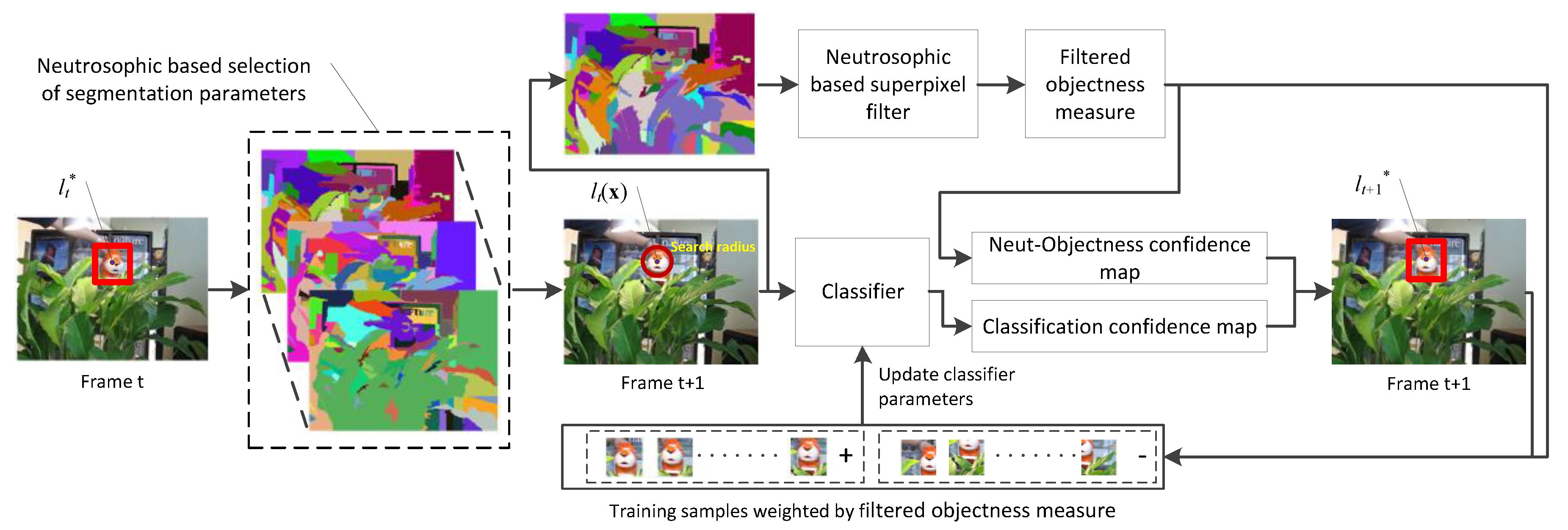
The basic flow of the online visual tracking of weighted multiple instance learning via neutrosophic similarity-based objectness estimation is shown in
Figure 1. Before the tracking process, the classifier of multiple instance learning is initialized with the same method as the weighted multiple instance learning [
15]. Suppose
is the center of the object location at frame
t, the object location is represented by a rectangular bounding box. To produce robust objectness [
19,
20] information for tracking,
N segmentation results of frame
t are firstly calculated by utilizing
N parameter tuples for segmentation. Then we used the SVNS-based segmentation parameter selection method to select the parameter tuple, which can achieve the best segmentation result for the representation of the object area. When the next frame arrives, we calculated its segmentation result by using the selected segmentation parameter tuple. Each region in the segmentation result corresponds to a superpixel. The neutrosophic set-based superpixel filter was employed to filter out the noisy superpixel when measuring the objectness. The sliding window method was used to calculate two confidence maps. The classifier confidence map was calculated based on the afore-trained classifier. The Neut-Objectness confidence map was calculated based on the filtered objectness measure. Finally, each maximum value of the two kinds of confidence maps was utilized to decide
, which is the center of the object location at frame
t+1. The scale of the rectangular bounding box was fixed in this work. To update the classifier parameters, the filtered objectness measure was applied for weighting the training samples. We first cropped
M positive instances within the circular region centering at
to form a positive bag
, and the distribution is symmetric, then
L negative instances were cropped from an annular region with radius
to form a negative bag
, where
is the location of instance
x at frame
t+1. The instances in the positive bag were weighted by the filtered objectness measure, and the negative instances were weighted equally. All the instances were represented by
W Haar-like features. Each Harr-like feature corresponded to a weak classifier. All the weighted instances were employed to train the
W weak classifiers, and finally
K weak classifiers were chosen for constructing a strong classifier
Hk. For each frame, we chose the updated
Hk as the new classifier for tracking. For a new arriving frame, the above procedures were repeated.
3.2. Objectness Measure
The objectness measure [
20] is always utilized in the research area of object detection for quantifying the degree of an image window containing an object. The color contrast, edge density, and superpixel straddling (SS) methods were proposed in [
20], and it has been proven that the SS measure is suitable for object tracking [
17]. The SS-based objectness for a window
Ow can be calculated by:
where
S(
Ti) is the superpixel set obtained by the literature [
21], with the segmentation parameter tuple
Ti. For each superpixel
s,
computes its area outside
Ow and
calculates its area inside
Ow. From Equation (1), we can get determine that a superpixel contributes less when it straddles the window
Ow. The superpixels inside the window
Ow contribute the most.
achieves to 1 when there is not any superpixel straddling the window
Ow.
As seen in Equation (1), the segmentation parameter tuple
Ti is also an important parameter.
Ti is a set of parameters that can affect the segmentation result greatly. Different segmentation algorithms always relate to different parameters. For the efficient graph-based image segmentation algorithm [
21] employed in this work, each tuple
contained three parameters including
(used to smooth the input image before segmenting it),
k (value for the threshold function), and
m (minimum component size enforced by post-processing). As shown in
Figure 2, when we use the same segmentation algorithm [
21] but employ different segmentation parameter tuples, the segmentation results are quite different. In addition, with the three different segmentation results, the corresponding superpixel sets are also quite different from each other. From Equation (1), we can find that the calculation of SS-based objectness highly depends on the shape and distribution of the superpixels in the image. To apply the objectness measure for weighting the training samples, we then proposed a neutrosophic set-based scheme to handle such a problem.
3.3. Neutrosophic Set-Based Segmentation Parameter Selection
To apply the objectness information for enhancing the tracker, a suitable segmentation parameter tuple should first be chosen. A well-built superpixel set is one of the most important preconditions for producing reliable objectness measures for the application of visual tracking. A well-built superpixel set should have the ability to enhance the objectness response at the object location. In addition, the symmetric surrounding information should also be considered seriously. The neutrosophic theory has shown its ability to deal with uncertain situations, and the neutrosophic similarity score between SVNSs is applied in this work.
The neutrosophic theory was firstly proposed by Smarandache [
22]. The original neutrosophic theory is difficult to use for tackling practical problems. SVNS [
33] is a subclass of the neutrosophic set with a finite interval, and it is proposed for practical usage. Let
, which denotes a set of alternatives. For a multiple criteria neutrosophic situation, the alternatives
Ai can be represented as:
where
is a set of criteria,
TCj(
Ai) denotes the degree to which the alternative
Ai satisfies the criterion
Cj,
ICj(
Ai) indicates the indeterminacy degree to which the alternative
Ai satisfies or does not satisfy the criterion
Cj,
FCj(
Ai) indicates the degree to which the alternative
Ai does not satisfy the criterion
Cj,
,
,
.
Suppose
is an ideal alternative with the criteria
Cj. The cosine similarity score between
Ai and
A* is defined by [
35]:
The corresponding tangent similarity score is defined as [
24]:
where
wj is the weight for each criterion, and
,
. Both the cosine and tangent measures have been successfully employed for medical diagnoses [
24] and some visual analysis missions [
7,
26]. In this work, the neutrosophic similarity score was utilized for fusing information, and these two measures were tested separately in the experimental section.
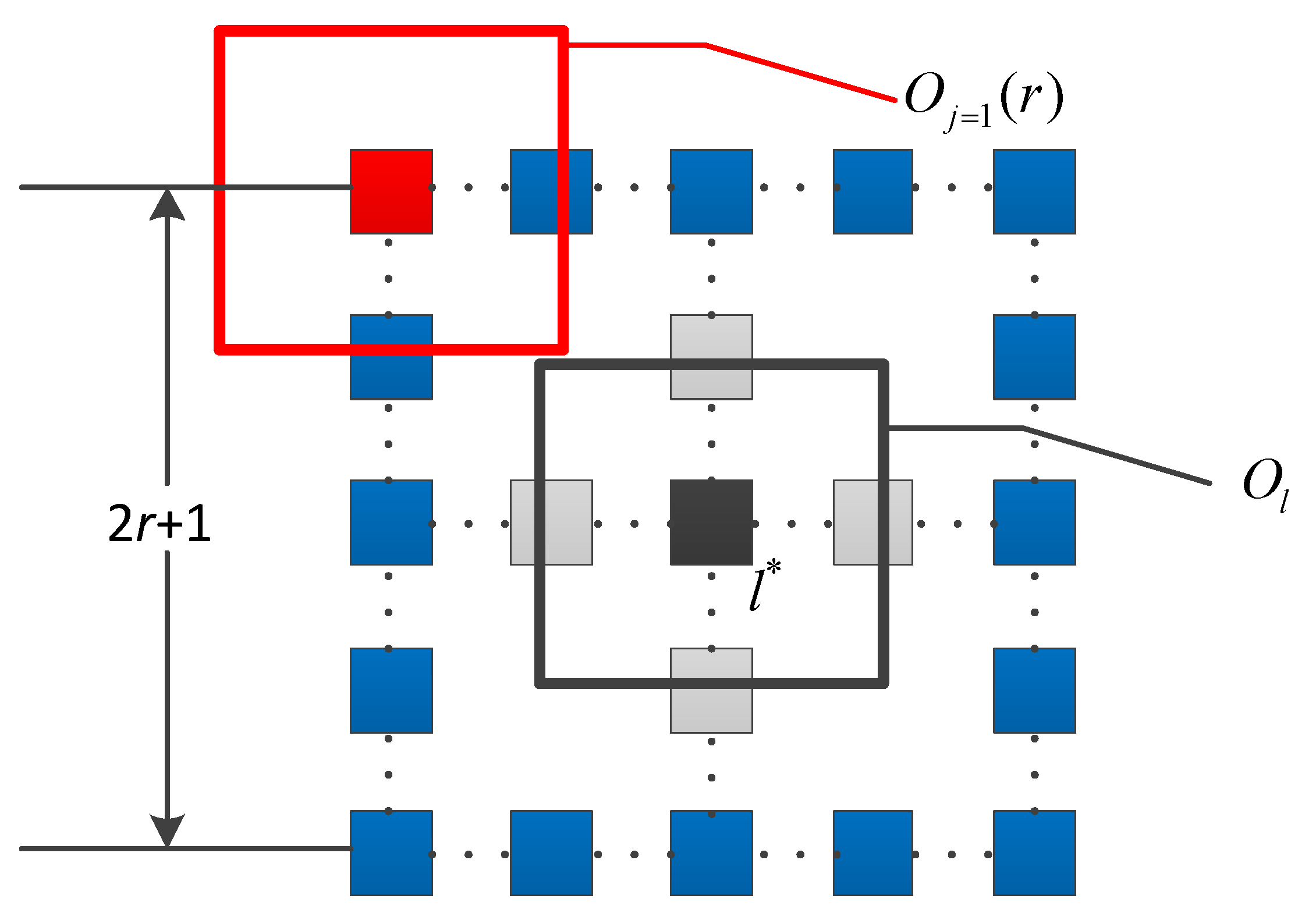
As we want to use the objectness measure to weight the training samples, the weights of the samples close to the object location should be enhanced. Considering such a problem, the object location objectness enhancing criterion was proposed. For the segmentation parameter tuple
Tk, the corresponding membership functions
TO(
Tk) (truth),
IO(
Tk) (indeterminacy), and
FO(
Tk) (falsity) were defined as:
where
Ol* is the rectangular window corresponding to the object location and
Ti is the the
i-th segmentation parameter tuple. As shown in
Figure 3,
is a square window centered at the
j-th pixel of the
C uniform sampled pixels on the boundary of the square window with the edge length of 2
r+1(pixel) centered at
l*, the distribution of
is symmetric,
l* is the center of the object location, and
has the same size as the objects.
Let
denote the ideal alternative with the object location objectness enhancing criterion. Substituting Equations (5)–(7) into Equation (3), we obtain the cosine similarity score between the choice of
Ti and the ideal choice:
When substituting Equation (5) into Equation (4), we obtain the corresponding tangent similarity score:
Suppose we have N segmentation parameter tuples waiting for selection, the tuple with the maximum similarity score is chosen as the right tuple Tsel. For the cosine and tangent measures, the selections may be different from each other.
3.4. Neutrosophic Set-Based Superpixel Filter
As shown in Equation (1) and
Figure 2, all the superpixels were taken into the consideration for the estimation of the objectness. However, such a simple method may bring in some noise for the objectness estimation. For instance, the superpixel far from the object or the superpixel that is too large size may disturb the objectness of the tracked object.
By considering the uncertain information, the intersection and shape–distance criteria were considered in this work. For the intersection criteria, the corresponding true, indeterminate, and faulty membership functions are defined as follows:
where
Ol is the rectangular window, which corresponds to the object location calculated by the afore-trained classifier before the modification, suppose
S(
Tsel) is the superpixel set obtained by the literature [
21] with the selected segmentation tuple
Tsel, and
si is the
i-th superpixel included in
S(
Tsel).
A superpixel is more likely to satisfy the intersection criteria when it is located in the estimated object location. The corresponding uncertain probability increases with the area outside the object location.
To enhance the robustness of the neutrosophic set-based method for judging a superpixel, the shape and the distance information were considered. Using the shape–distance criteria, we can further give the definitions:
where
wsi and
hsi are the width and height, respectively, of the tight rectangular bounding box of the super pixel
si,
wol and
hol are the width and height corresponding to the object window
Ol,
xsi is the centroid location of
si,
l is the center of the
Ol, and
D is half the length of the
Ol diagonal. The function
f(
x) in
Tsd(
i) is defined as:
The domain of
f(
x) is positive real numbers, and then
f(
x) is manually designed for the purpose of decreasing the value of
Tsd(
i) when the width or the height of
si is larger or smaller than the
wol or
hol. As seen in
Figure 4, when
x > 1, the response of
f(
x) decreases slowly in the intervals of [1,1.2] and [1.6,1.8], but decreases sharply during the interval of [1.2,1.6]. The reason for such a design is that we wanted to keep the information of those superpixels with a relative similar size to the object, and try to discard the superpixels with a much larger width or height than the object. As shown in
Figure 4, the response has decreased at the value of less than 0.1 when
x equals 1.6. However, we choose a different solution when
x < 1. The response of
f(
x) decreases much slower than in the interval of
x > 1, because a small superpixel may be one of the real parts of the object. We tried to keep the information of such superpixels.
As seen in Equation (13) and Equation (14), the shape factor is mainly considered when calculating the truth response, and the distance factor is primarily considered as the indeterminate information.
Let
denote the ideal alternative with the intersection and shape–distance criteria. Substituting Equations (10)–(16) into Equation (3), we obtain the cosine similarity score between the choice of
si and the ideal superpixel:
where
,
. When substituting Equation (5) into Equation (4), we obtain the corresponding tangent similarity score:
where
,
.
By employing the similarity score, we finally give the definition of the neutrosophic set-based superpixel filter:
where
Hi is the filter response for the superpixel
si,
γ is a threshold parameter, and
ls(
i) is the cosine or tangent similarity score calculated by Equation (17) or Equation (18).
The results of the superpixel filter are applied for estimating the neutrosophic set-based objectness, then the definition of the filtered objectness measure is given by:
where
S(
Tsel) is the superpixel set obtained by using the selected segmentation parameter tuple
Tsel and
OW is a rectangular window with the same size as the object.
3.5. Object Localization
For the task of visual tracking, the precision of the object location given by the tracker is very important for the following tracking procedure. An inaccurate location may disturb the updating of the classifier, and the tracking result may drift from the real object location in the following frames, even leading to failure. To improve the robustness of the object localization, both the Neut-Objectness confidence map and the classification confidence map were employed in this work.
The classification confidence map is calculated by using the afore-trained classifier Hk. All the windows whose center is located within the circle area for searching are employed as candidates, suppose sr denotes the searching radius. The scale of each window is the same as the tracked object. The Hk response of each candidate window finally forms the classification map.
The neutrosophic-based objectness measure is utilized to modify the location
l, which fully depends on
Hk. We calculated the Neut-Objectness confidence map by using the similar manner of the calculation of the classification confidence map, but the response of the filtered objectness measure is employed instead of the
Hk response. Let
lnss denote the center location of the candidate window with a maximum value within the Neut-Objectness confidence map, and the corresponding response is
nss(
Ow(
lnss),
Tsel). The fused object location is calculated by
where
l denotes the location, corresponding to the center of the candidate window with the maximum value within the classification confidence map,
Hk(
lnss) is the response of
Hk for the window centered at
lnss,
λ is the ratio parameter, and
τ1 and
τ2 are threshold parameters for
λ,
τ1,
τ2∈[0,1].
As seen in Equation (21), we modify the location calculated by the afore-trained classifier only when the maximum of the Neut-Objectness confidence map and the Hk response at the corresponding location achieves a relative high value. Such a method can effectively remove the interference, which may be caused by an objectness estimation that is not stable enough.
3.6. Weighted Multiple Instance Learning
In this work, we considered the importance of the instances in the positive bag
X+ during the learning process. The weight of the
j-th positive instance in
X+ is obtained by using the filtered objectness measure:
where
OWj is the window corresponding to the
j-th instance in
X+. Then, the positive bag probability is computed by [
15,
17]:
where
is the posterior probability for the positive sample
x1j, and
x1j denotes the
j-th instance in the positive bag.
Comparing the weight methods employed in WMIL [
15] and ONMIL [
17], we used the neutrosophic set-based objectness measure to calculate the weight of each positive instance. In the WMIL tracker, the weight is computed mainly based on the Euclidean distance between the center of the instance and the estimated object location. When the tracking result drifts from the real object location, those real positive instances will be assigned as a relative low weight because of the long distance, which is contrary to the fact. For the ONMIL tracker, the traditional objectness estimation with superpixel straddling [
20] is directly employed as the weight of each instance. As we have discussed above, the traditional objectness estimation is highly relevant to the segmentation results. When the scene changes during the tracking process, a weak objectness measure may be obtained if an inappropriate set of superpixels is used. In addition, for the task of visual tracking, some superpixels may also disturb the objectness response of the tracked object area. In our method, we first employed an online selection method of segmentation parameter tuples to produce a well-built result of a superpixel set. Secondly, we proposed a neutrosophic set-based superpixel filter to enhance the objectness estimation for the tracking application. Finally, when calculating the weight for each instance, the filtered objectness measurements were utilized for weighting when the corresponding response results were robust enough.
The posterior probability of labeling
xij to be positive is defined as [
13]:
where
i∈{0,1}, as has been mentioned above,
x1j denotes the
j-th instance in the positive bag,
x0j denotes the
j-th instance in the negative bag, and σ is the sigmoid function,
.
The strong classifier
Hk in Equation (24) is defined as:
where
f(
xij) is a set of Haar-like features corresponding to the weak classifier
hk(
xij),
f(
xij) = (
f1(
x),…,
fK(
x))
T. We assume the features in
f(
xij) are independent and assume uniform prior p(y = 0) = p(y = 1) as MIL tracker [
13]. Then, the
hk(
xij) is described as [
13]:
The conditional distribution in
hk(
.) is also defined as a Gaussian function as the MIL tracker, that is:
Like the WMIL tracker [
15], the parameters
and
are updated as follows:
where
is the learning rate,
M is the number of positive samples, and
is the average of the
k-th feature extracted from the
M positive samples. The parameters
and
are updated by employing the same rules.
Similar to the WMIL tracker, the bag log-likelihood function is defined as [
15]:
where
L is the number of negative samples,
wj is the weight of the
j-th positive instance defined in Equation (22),
yi is the label of the training bag,
yi equals to 1 when the bag is positive, and
yi is set as 0 when the bag is negative.
As the method utilized in MIL [
13], WMIL [
15], and ONMIL trackers [
17], our tracker maintains
W weak classifiers in the pool
. At each frame, the
K weak classifier with strong classification ability is selected to form
Hk. In the WMIL tracker, a more efficient criterion was proposed. Similar rules are employed here. The scheme for selecting K weak classifier is given below [
15].
where [
15]:
where
wj and
wm are the weights of the corresponding samples, and they are calculated by Equation (22).
Finally, the main steps of the proposed NeutWMIL tracker are shown in Algorithm 1.
| Algorithm 1 Online neutrosophic similarity-based objectness tracking with weighted multiple instance learning algorithm (NeutWMIL) |
Initialization:
(1) Initialize the region of the tracked object in the first frame.
(2) Initialize the MIL-based classifier Hk by employing the training bags surrounding the object location.
Online tracking:
(1) Select suitable segmentation parameter tuple Tsel by utilizing the method of neutrosophic set-based segmentation parameter selection.
(2) Read a new frame of the video sequence.
(3) Calculate the superpixel set for the current frame with the selected tuple Tsel.
(4) Compute the estimation of the filtered objectness surrounding the location obtained by the afore-trained classifier Hk, and get the final object location l* in this frame by Equation (21).
(5) Compute the neutrosophic set-based weight by Equation (22).
(6) Crop M positive instances within the circular region centering at to form a positive bag, then crop L negative instances from an annular region to form a negative bag.
(7) Update the parameters of W weak classifiers by Equation (28).
(8) Select K weak classifiers by Equation (30) and form the current classifier Hk.
(9) Go to step (1) until the end. |
4. Experiments
In this section, we compared the proposed NeutWMIL tracker with six trackers on 20 challenging video sequences. The six trackers were the NeutanWMIL, ONWMIL, WMIL [
15], MIL [
13], OAB [
10], and SemiB[
11] trackers. Specifically, the NeutWMIL and the NeutanWMIL trackers were two kinds of the proposed tracking algorithm. The only difference is that the NeutWMIL tracker employed the cosine similarity measure, and the NeutanWMIL tracker used the tangent measure when the neutrosophic similarity estimation was needed during the tracking process. For the ONWMIL tracker, we implemented it using a similar instance weighting method to that proposed in [
17]. The objectness estimation was directly applied for weighting each instance for the ONWMIL tracker, and the segmentation parameters were kept constant. The instance-weighting scheme was the only difference when compared with the NeutWMIL and the NeutanWMIL trackers. The source codes of the WMIL, MIL, OAB, and SemiB trackers are all publicly available, and the default parameter settings were utilized.
4.1. Parameter Setting
For the NuetWMIL, NeutanWMIL, and ONWMIL trackers, all the parameters related to the WMIL tracker were set as they are mentioned in the publicly available source codes. For instance, we set , the search radius sr was set to 25, and ws set to 1.5sr, the number of the cropped negative instances L was set to 50, the number of the weak classifiers W = 150, and the strong classifier Hk maintained K = 15 weak classifiers. Three segmentation parameter tuples were chosen—, , and . When we performed the tuple selection algorithm, the parameter r defined in Equation (6) was set to 8, and C was set to 4, which means the four corners of the square window with an edge length of 17 pixels were considered for evaluating the indeterminate estimation. For the neutrosophic set-based superpixel filter, when calculating the similarity score of each superpixel by Equations (17)–(18), we set wcint = wcsd = wtint = wtsd = 0.5, which meant each criterion was treated equally. The threshold parameter in Equation (19) decided how many superpixels could pass the filter. To fully use the superpixel information and to filter the noisy superpixel in the meantime, a near median value 0.4 was set to . For the object location step, the location estimated by the trained classifier was more robust than the filtered objectness-based result statistically. However, when a relatively high response of the filtered objectness was received, as well as the response of the classifier, the objectness results were usually robust enough, and a more accurate result could be achieved by fusing these two kinds of results. By considering this, for the parameters in Equation (21), we set and , and then the fusing ratio is set to 0.3. Finally, all parameters were kept constant for all the experiments.
4.2. Evaluation Criteria
We used two kinds of evaluation criteria, one was center location error, and the other was the success ratio based on the overlap metric. For the center location error metric, the Euclidean distance between the estimated object location and the manually labeled ground truth was considered. The overlap score is defined as:
where
is the object area estimated by the tracker in the
i-th frame,
ROIi corresponds to the ground truth. Giving a threshold
u, we can say the result is correct if
pi >
u. Suppose
FNs is the number of the frames, then the success ratio is calculated by:
where:
4.3. Quantitative Analysis
Details of each tested video sequence are given in
Table 1. 14,163 frames are evaluated here. The challenge degree grew with the increase in the NC value. The average center location errors for the tested trackers are shown in
Table 2. We can see that the NeutWMIL tracker ran the best in 13 sequences, and it performed the second best in four sequences. The NeutanWMIL tracker performed the best in four sequences and the second best in six sequences. The results of the corresponding average overlap ratio are given in
Table 3. We can see the NeutWMIL tracker had the best performance in 12 sequences and the second best in six sequences. The NeutanWMIL tracker performed the best in five sequences and the second best in eight sequences.
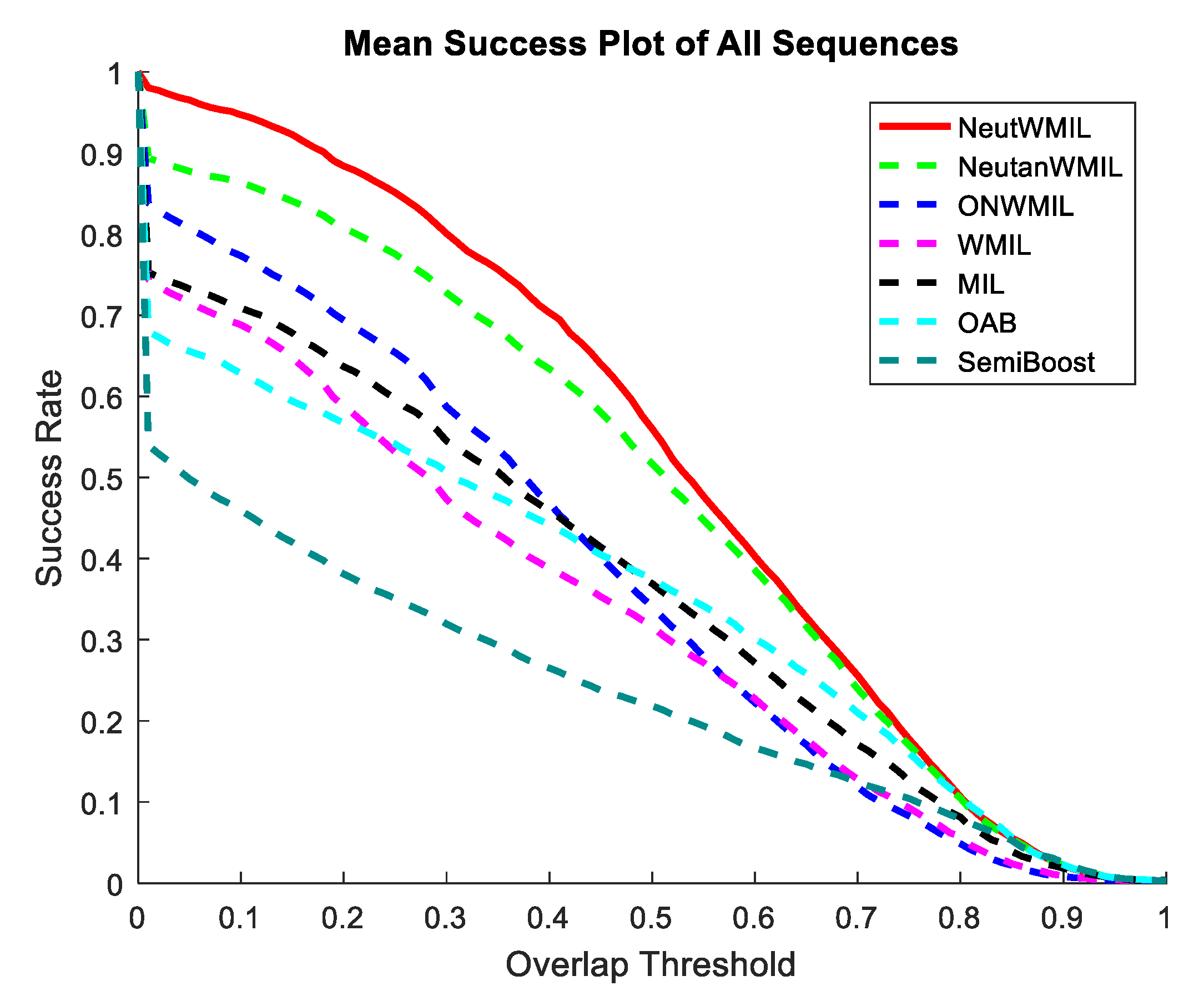
Figure 5 shows the plot of average success of the evaluated trackers through all the sequence. We can see that the NeutWMIL tracker performed the best, and the NeutanWMIL tracker had the second best performance. We can also find that there is a big gap between the NeutWMIL tracker and the WMIL tracker, as well as the MIL tracker. Based on the last line of both
Table 2 and
Table 3, a conclusion can also be drawn that the proposed NeutWMIL tracker performs the best, and the proposed NeutanWMIL tracker performs the second best.
4.4. Qualitative Analysis
We chose thirteen representative sequences among the tested sequences for the Qualitative analysis. As seen in
Table 1,
Table 2 and
Table 3, the names of the selected 13 sequences are shown in bold font in each table. Based on the challenge degree of these sequences, they were separated into three groups for analysis. The success and center position error plots for each sequence can be seen in
Figure 6,
Figure 7 and
Figure 8. Some sampled tracking results are shown in
Figure 9,
Figure 10 and
Figure 11.
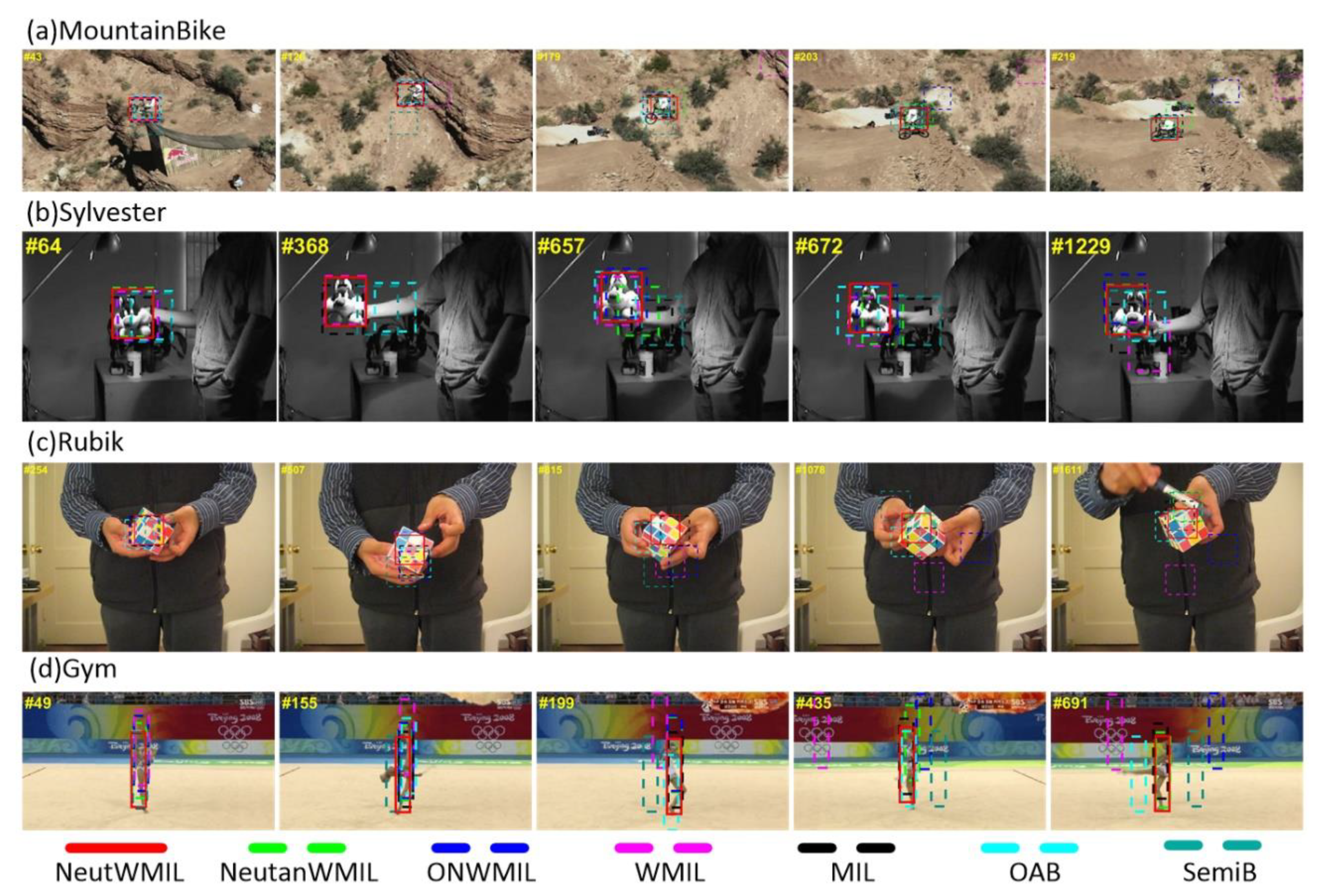
4.4.1. MountainBike, Sylvester, Rubik, and Gym
As shown in
Table 1, the first two sequences were with three types of challenges. The main challenges were in-plane and out-plane rotation, and there was a background clutter challenge in the
MountainBike sequence, and illumination variation challenge in the
Sylvester sequence. As seen in
Figure 9a, the SemiB tracker yielded a severe drift problem at frames #43, #126, and #179. The WMIL tracker failed due to the background clutter, as shown by frames #126 and #179. When the biker passed by the area with more challenging background clutter, the NeutanWMIL and ONWMIL trackers produced wrong object locations, as seen in frame #219. The OAB and SemiB trackers drifted away on account of the in-plane and out-plane challenge, as shown by frames #64 and #368 in
Figure 9b. Due to the rotation and illumination variation challenges, the trackers drifted from the object except the NeutWMIL tracker, as shown by frames #657 and #672. The center position errors of all the trackers at each frame are shown in
Figure 6. We can see the NeutWMIL tracker outperformed all the others, the results in
Table 2 and
Table 3 also support this conclusion. For the last two sequences, besides the scale variation, in-plane and out-plane rotation challenges, the occlusion was another challenging issue for the
Rubik sequence. For the
Gym sequence, there was also a deformation challenge. All the trackers drifted away due to the in-plane and out-plane rotation, as shown by frames #254, #507, #815, and #1078 in
Figure 9c, except the NeutWMIL and NeutanWMIL trackers. As shown in
Figure 6, the plot of center position error shows that NeutanWMIL tracker performed well until fame #1600, and the drift was mainly caused by the occlusion, as shown by frame #1611. Considering the deformation challenge, all the trackers except the NeutWMIL tracker were affected in some degree in the
Gym sequence. Drifts can be seen in
Figure 9d, the plot in
Figure 6 also reveals the drift problem.
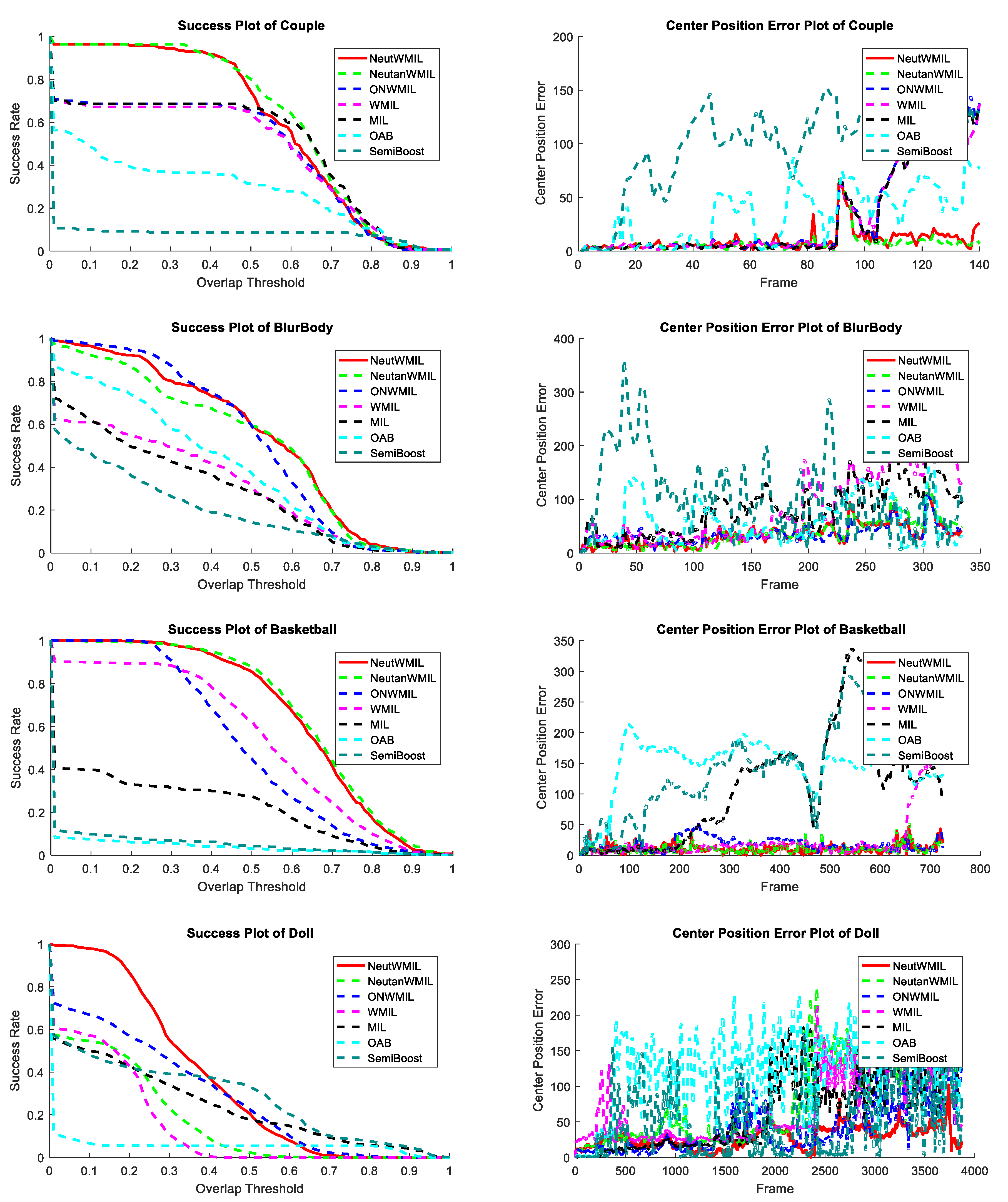
4.4.2. Couple, BlurBody, Basketball, and Doll
This group of sequences was more challenging than the previous one. The fast motion of the camera and background clutter were the most challenging problems in the
Couple sequence. As shown in
Figure 7,
Table 2, and
Table 3, the NeutanWMIL tracker performed the best in the
Couple sequence. The OAB and SemiB trackers could not adaptively adjust to these challenges, and they drifted from the ‘couple’, as shown in
Figure 10a. As seen in
Figure 7, we can see that all the trackers drifted away severely near frame #90, because a very fast motion occurred to the camera. However, as shown in
Figure 10a, the ‘couple’ was re-tracked by the NeutWMIL and NeutanWMIL trackers. For the
BlurBody sequence, besides the fast motion, the most challenging problems were motion blur and scale variation. As shown in
Figure 7, the SemiB tracker drifted away at the very beginning. The related screenshots can be seen by frames #12 and #16 in
Figure 10b. As shown by frames #124 and #203, the WMIL, MIL, and OAB trackers drifted for the scale variation and motion blur challenges. From the plots shown in
Figure 7, we can find that the NeutWMIL and NeutanWMIL trackers performed the best, the ONWMIL tracker also performed well to some extent. There was background clutter, out-plane rotation, deformation, and scale variation challenges in the
Basketball sequence. The OAB and SemiB trackers failed quickly when a player appeared nearby the target, as shown by frame #39 in
Figure 10c. The MIL tracker also drifted from the target player after he passed by several other players, as shown by frames #258 and #468. The WMIL tracker ran well until the player passed by several other players with similar color, as shown by frame #664. As shown in
Figure 7,
Table 2, and
Table 3, the NeutanWMIL tracker ran the best for both the
BlurBody and
Basketball sequences, but the gap between the NeutanWMIL tracker and the NeutWMIL tracker is very small. Challenges like illumination variation, scale variation, occlusion, and rotation were included in the
Doll sequence. The WMIL, OAB, and SemiB trackers drifted away quickly, as shown by frames #185, #225, and #742. The NeutanWMIL and ONWMIL trackers could not adaptively adjust to these challenges and drifted from the doll, as shown by frames #1414 and #2324. The proposed NeutWMIL tracker can yield more stable and more accurate results than the other six trackers.
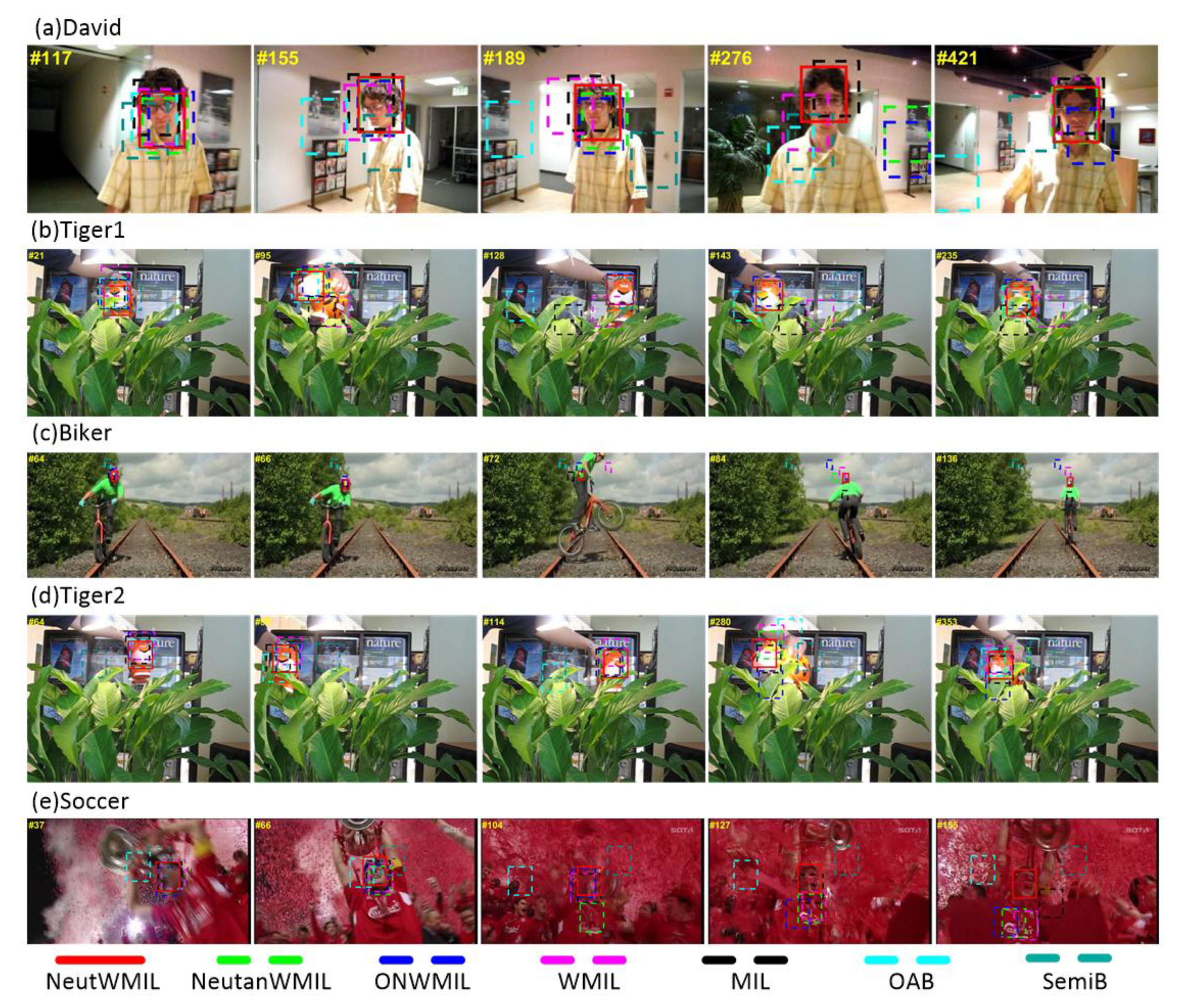
4.4.3. David, Tiger1, Biker, Tiger2, and Soccer
This group had the most challenging sequences. Seven types of challenge were included in the
David sequence. Details can be seen in
Table 1. The OAB tracker was distracted by the wall because of the similar color, the SemiB tracker drifted from the target mainly due to the challenge of illumination variation, as shown by frames #117 and #155 in
Figure 11a. The NeutanWMIL and ONWMIL trackers were also distracted by the wall because of the illumination change and the scale variation, as well as the similar texture between the painting and the target. As seen in
Figure 7,
Figure 11a,
Table 2, and
Table 3, the NeutWMIL tracker produced a more robust estimation of object location. For the sequences of
Tiger1 and
Tiger2, seven types of challenge were included in the
Tiger1 sequence, and
Tiger2 consisted of eight types of challenge. The SemiB, OAB, WMIL, MIL, and ONWMIL trackers could not adjust to these challenges well, as shown by frames #21, #95, #128, #143, and #235 in
Figure 11b, as well as frames #64, #99, #280, and #353 shown in
Figure 11d. The performance gap between the NeutanWMIL tracker and the NeutWMIL tracker was very small in the sequences of
Tiger1 and
Tiger2, as shown in
Figure 7,
Table 2, and
Table 3. The
Biker sequence mainly contained challenges like fast motion, scale variation, out-plane rotation, out of view, and low resolution. The OAB and SemiB trackers drifted from the target mainly due to the challenges of scale variation and head rotation, as shown by frames #64 and #66 in
Figure 11c. All the trackers failed nearby frame #70, because of a very fast move from the target, as shown by frame #72 in
Figure 11c. However, the NeutanWMIL and NeutWMIL trackers snapped to the target again when the target was located within the searching area, as shown by frames #84 and #136. The
Soccer sequence had the most challenging problems among the tested sequences. As shown by frame #37 in
Figure 11e, the OAB and SemiB trackers drifted away because of the challenges of motion blur and rotation. As seen in
Figure 8, we can find the estimation results of the NeutWMIL and NeutanWMIL trackers were not stable between the frame #70 and #120. This is mainly due to the severe occlusion during such a period. The ONWMIL, WMIL, and MIL trackers drifted away after such a long-term occlusion. When the target appeared, the NeutWMIL snapped to the target again, and performed the best in the following frames, as shown by frames #127 and #155.
4.5. Discussion
With the above analysis, we can find that the proposed NeutWMIL tracker had the best performance. This was mainly due to three contributions of this work. First, by employing the proposed object location objectness enhancing criterion, a more appropriate tuple of segmentation parameter was selected, and then a more suitable superpixel set for measuring the objectness was produced, which helped the tracker to adjust for different scenes during the tracking process. Secondly, the intersection and shape–distance criteria were proposed for constructing the superpixel filter, which helped the tracker filter out those superpixels which may disturb the tracker, and more reliable sample weights were produced for updating the classifier. Thirdly, the object location was finally decided by fusing the information of the Neut-Objectness confidence map and the classification confidence map, which could also enhance the robustness of the tracker.
As shown in
Figure 5,
Table 2, and
Table 3, we can see that there is a big gap between the proposed NeutWMIL and the WMIL tracker. The main reason for this is the NeutWMIL tracker utilized the neutrosophic set-based objectness weighting algorithm. Weights that are more robust can be produced when there is a small drift from the real object location. The comparison result also shows that the NeutWMIL tracker performed better than the NeutanWMIL tracker. As we have mentioned, the only difference between these two trackers is the usage of different neutrosophic similarity measures. The cosine similarity measure is applied for the NeutWMIL tracker, and the tangent similarity measure is employed by the NeutanWMIL tracker. Regarding Equations (8) and (9) and Equations (17) and (18), it can be found that the truth element is enhanced for the cosine measure, and the I and F elements are only applied for decreasing the similarity response. Such a scheme seems more suitable for the judging application in this work. However, all the T, I, and F elements are treated equally for the tangent measure. As shown in
Figure 5,
Table 2, and
Table 3, a relatively big gap exists between the NeutWMIL tracker and the ONWMIL tracker. This result reveals that the proposed weighting method contributed much more to the tracker, rather than using the objectness estimation directly.


