Intuitionistic Type-2 Fuzzy Set and Its Properties

Abstract

Decision making under uncertainty describes situations that consider a profound lack of knowledge, where the functional form is completely unknown, and often, the relevant input and output variables are unknown as well. Data, being the vital input of decision making, contain a dissimilar level of imprecision that necessitates different approaches for making a proper and legitimate decision. In this article, we propose the concept of the intuitionistic type-2 fuzzy set (IT2FS). Several arithmetic operations on IT2FS such as union, intersection, complement, containment, etc., are defined, and the related algebraic properties of IT2FS are also studied. Subsequently, we define two new operators, namely the necessity operator and the possibility operator, to convert an IT2FS into an ordinary T2FS, and then discuss some of their basic properties. Moreover, in this study, two distance measures, the Hamming distance and Euclidian distance of IT2FS, are proposed, and their applications are illustrated with an example.

1. Introduction

Uncertainty is an intrinsic feature of information. In many scientific and industrial applications, we make decisions in an environment with different kinds of uncertainty. Currently, most of the decision-making processes involve retrieving and analyzing information, which is mostly incomplete, noisy, fragmentary, or sometimes contradictory. Therefore, the models characterizing the real world require being accompanied by the proper uncertainty representations. With the advent of soft computing (SC) methods, several powerful tools in the field of computational intelligence were introduced including type-1 fuzzy logic, neural networks, evolutionary algorithms, and hybrid intelligent systems [1,2,3].

The application of fuzzy sets in decision making and optimization problems has been widely studied since its inception [4]. However, in the literature, many studies have shown growing interest in the study of decision-making problems using intuitionistic fuzzy sets/numbers [5,6]. The intuitionistic fuzzy set (IFS) is an extension of the fuzzy set introduced by Atanassov [7,8]. IFS is a more generalized version of the fuzzy set, which can be defined in terms of the degrees of membership and non-membership (the residual term is referred to as the degree of indeterminacy). Presently, IFSs are being studied and used in different fields of science and technology for decision making problems. For instance, Marasini et al. [9] implemented an IFS approach for the problem of students’ satisfaction with university teaching, which can take into account a source of uncertainty related to items and another related to subjects. Subsequently, Marasini et al. [10] presented a study, where the intuitionistic fuzzy set was used for questionnaire analysis, with a focus on the construction of membership, non-membership, and uncertainty functions. In addition, several researchers have developed several decision-making problems in the field of intuitionistic fuzzy sets [11,12,13,14,15,16].

A type-2 fuzzy set (T2FS) is an extension of the ordinary fuzzy set, i.e., type-1 fuzzy set (T1FS). The fundamental superiority of the type-2 fuzzy set, over the type-1 fuzzy set, has been its ability to capture the membership of relevant membership values, where the uncertainty is handled more accurately. The membership value of a type-1 fuzzy set is a real number in [0, 1]. On the other hand, the membership value of a T2FS is a type-1 fuzzy set. The concept of T2FS was introduced by Zadeh [17,18,19]. The overviews of type-2 fuzzy sets were given in Mendel [20]. Since ordinary fuzzy sets and interval-valued fuzzy sets are special cases of type-2 fuzzy sets, Takac [21] proposed that type-2 fuzzy sets are very practical in the circumstances where there are more uncertainties. Kundu et al. [22] proposed a fixed charge transportation problem with type-2 fuzzy parameters from the viewpoint of type reduction and the centroid. Mizumoto and Tanaka [23,24] and Dubois and Prade [25] investigated the logical operations of T2FS. Later, many researchers did many investigations on theoretical [26,27,28,29], as well as on various application domains [30,31,32,33,34] of T2FS.

Considering both intuitionistic fuzzy and type-2 fuzzy environments, Singh and Garg [35] proposed the symmetric TIT2 fuzzy set to develop some new interval type-2 (IT2) intuitionistic fuzzy aggregation operators, which can consider the multiple interactions between the input arguments. Subsequently, Garg and Singh [36] proposed triangular interval type-2 intuitionistic fuzzy sets (TIT2) and their three aggregation operators: TIT2 intuitionistic fuzzy weighted averaging, TIT2 intuitionistic fuzzy ordered weighted averaging and TIT2 intuitionistic fuzzy hybrid averaging based on Frank norm operation laws. However, in spite of the existing works on interval type-2 intuitionistic fuzzy sets, in the literature, to the best of our knowledge, there does not exist any study on generalized the intuitionistic type-2 fuzzy set. Therefore, to circumvent this gap in the literature, in this study, we introduce the concept of the generalized intuitionistic type-2 fuzzy set (IT2FS) whose type-1 membership is the ordinary fuzzy membership, and the resulting type-2 consists of both membership and non-membership as the intuitionistic fuzzy set. We introduce the notions of basic set operations and focus on the algebraic properties of these sets with several illustrative examples. Further, we define two operators on the set whose basic function is to convert an IT2FS into an ordinary T2FS and also describe some properties of these operators. Finally, we define two distance measures, the Hamming distance and Euclidian distance, of IT2FS, which are illustrated with a numerical example. The main contribution of this article is highlighted as follows.

(i)

The concept of a generalized intuitionistic type-2 fuzzy set is proposed.

(ii)

Some set-theoretic operations including the union, intersection, and complement of IT2FS are presented.

(iii)

Several properties of IT2FS like $idempotency$, $commutative$, $associative$, $distributive$, $involution$ and $De Morgan’s law$ are proposed.

(iv)

Possibility and necessity operators of IT2FS are investigated.

(v)

Two distance measures, the Hamming distance and Euclidian distance, are proposed in this study.

(vi)

A suitable application based on a medical diagnosis system is presented, where the distance measures of IT2FS are used.

The rest of the paper is organized as follows. The preliminary concepts of our study are presented in Section 2. In Section 3, we propose the intuitionistic type-2 fuzzy set (IT2FS) and give examples. The geometrical interpretation of IT2FS is shown in Section 4. Subsequently, in Section 5, some set-theoretic operations of IT2FS including union, intersection, and complement are defined. In Section 6, some properties of IT2FS like $idempotency$, $commutativity$, $associativity$, $distributive$, $involution$, and $De Morgan’s law$ are verified. In Section 7, the necessity and possibility operators of IT2FS are defined. Successively, in Section 8, two distance measures of IT2FS are defined, and an example, illustrating the application of these distance measures in a real-life application based on a medical diagnosis system, is presented in Section 9. Finally, the conclusion of the study is drawn in Section 10.

2. Preliminaries

Before introducing the new concept of IT2FS, we first present some essential concepts and notations of T2FS and IFS.

2.1. Type-2 Fuzzy Set

A type-2 fuzzy set (T2FS) is a fuzzy set whose membership degree includes uncertainty, i.e., the membership degree is a fuzzy set and not a crisp set. A T2FS $\tilde{A}$ is defined as (Mendel and John [37]):

$$\tilde{A}=\left\{\left(\left(x, u\right), {\mu }_{\tilde{A}}\left(x,u\right)\right):\forall x\in X, \forall u\in J_x\subseteq \left[0, 1\right]\}\right\},$$

where 0 ≤ ${\mu }_{\tilde{A}}\left(x,u\right)$ ≤ 1 is the secondary membership function and ${\mathrm{J}}_{\mathrm{x}}$ is the primary membership of $\mathrm{x}\in \mathrm{X}$, which is the domain of ${\mathsf{\mu }}_{\tilde{\mathrm{A}}}\left(\mathrm{x},\mathrm{u}\right)$. Alternatively, $\tilde{\mathrm{A}}$ can be expressed as:

$$\tilde{A}={\int }_{x\in X}\left({\int }_{u\in J_x}{\mu }_{\tilde{A}}\left(x,u\right)/u\right)/x, J_x\subseteq \left[0,1\right],$$

where ${\displaystyle \int }{\displaystyle \int }$ denotes union over all admissible $x \mathrm{and} u$. For the discrete universe of discourse, ${\displaystyle \int }$ is replaced by ${\displaystyle \sum }$. For each value of $\in X$, the secondary membership function ${\mu }_{\tilde{A}}\left(x,u\right)$ is defined as:

$${\mu }_{\tilde{A}}\left(x,u\right)={\int }_{u\in J_x}{\mu }_{\tilde{A}}\left(x,u\right)/u,$$

where for a particular $u=u^{\prime }\in J_{\mathrm{x}},{\mu }_{\tilde{A}}\left(x,u^{\prime }\right)$ is called the secondary membership grade of ($x$,$u^{\prime }$).

Example 1.

Let the set “young” be represented by a T2FS $\tilde{A}$. The “youthness” is the primary membership function of$\tilde{A}$and the “degree of youthness” is the secondary membership function. Let$X= \left\{8, 10, 14\right\}$be an age set with the primary membership of the points of$X$respectively$J_8$= $\left\{0.8, 0.9, 1.0\right\}$,$J_{10}$= $\left\{0.6, 0.7, 0.8\right\}$, and$J_{14}=\left\{0.4, 0.5, 0.6\right\}$. The secondary membership function of the point 8 is:

$${\tilde{\mu }}_{\tilde{A}}\left(8, u\right)= \left(0.9/0.8\right)+ \left(0.7/0.9\right)+ \left(0.6/1.0\right),$$

i.e.,${\tilde{\mu }}_{\tilde{A}}\left(8, 0.8\right)= 0.9$is the secondary membership grade of 8 with the primary membership grade 0.8.

Similarly,

$${\tilde{\mu }}_{\tilde{A}}\left(10, u\right)=\left(0.8/0.6\right)+ \left(0.7/0.7\right)+ \left(0.6/0.8\right)\mathrm{and}{\tilde{\mu }}_{\tilde{A}}\left(14, u\right)=\left(0.9/0.4\right)+ \left(0.8/0.5\right)+ \left(0.5/0.6\right).$$

Accordingly, discrete T2FS$\tilde{A}$can be represented as:

$$\begin{array}{c}\tilde{A}=\left(0.9/0.8+0.7/0.9+0.6/1.0\right)/8+\left(0.8/0.6+0.7/0.7+0.6/0.8\right)/10\\ + \left(0.9/0.4 +0.8/0.5 + 0.5/0.6\right)/14.\end{array}$$

2.2. Intuitionistic Fuzzy Set

The classical fuzzy set is a set with a membership function, but an intuitionistic fuzzy set (IFS) is a set that has a membership function, as well as a non-membership function. According to Atanassov [7,8], an intuitionistic fuzzy set $A$ in $X$ is defined as an object of the following form.

$$A=\left\{x, {\mu }_A\left(x\right), {\gamma }_A\left(x\right):\mathrm{x}\in X,{\mu }_A\left(x\right)\in \left[0,1\right],{\gamma }_A\left(x\right)\in \left[0,1\right]\right\},$$

where the functions,

$${\mu }_A:X\to \left[0,1\right]$$

and:

$${\nu }_A:X\to \left[0,1\right]$$

define the degree of membership and the degree of non-membership respectively such that:

$$0\le {\mu }_A\left(x\right)+{\nu }_A\left(x\right)\le 1\mathrm{for}\mathrm{all}x\in X.$$

For the discrete universe of discourse, an IFS can be represented as:

$${\displaystyle \sum _{x\in X}} ({\mu }_A\left(x\right),{\nu }_A\left(x\right))/x.$$

According to this concept, every discrete ordinary fuzzy set may be written as:

$${\displaystyle \sum _{x\in X}} ({\mu }_A\left(x\right), 1-{\mu }_A\left(x\right))/x,$$

where ${\mu }_A$ is the membership function of the fuzzy set $A$. For continuous IFS, the ${\displaystyle \sum }$ is replaced by ${\displaystyle \int }$.

Example 2.

Let the set young be represented by the intuitionistic fuzzy set$A$. The degree of youthness and the degree of adultness are the membership and non-membership function, respectively. Let$X= \left\{12, 15, 17\right\}$and the membership grade of the point 12 be${\mu }_A\left(12\right)=\left\{0.7, 0.8, 0.9\right\}$, and the non-membership grade of the point 12 is${\nu }_A\left(12\right)=\left\{0.1, 0.2, 0.0\right\}$.

Similarly, let${\mu }_A\left(15\right)=\left\{0.6, 0.7, 0.8,\right\}$, ${\nu }_A\left(15\right)= \left\{0.4, 0.2, 0.1\right\}$,${\mu }_A\left(17\right)=\left\{0.4, 0.5, 0.6\right\}$, ${\nu }_A\left(17\right)=\left\{0.5, 0.3, 0.2\right\}$.

Therefore, the discrete intuitionistic fuzzy variable$A$ is represented as:

$$\begin{array}{l}A=\left(\left(0.7, 0.1\right) + \left(0.8, 0.2\right) + \left(0.9, 0.0\right)\right)/12 + \left(\left(0.6, 0.4\right) + \left(0.7, 0.2\right) + \left(0.8, 0.1\right)\right)/15\\ \hspace{1em}\hspace{1em}\hspace{1em}\hspace{1em}\hspace{1em}\hspace{1em}\hspace{1em}+ \left(\left(0.4, 0.5\right) + \left(0.5, 0.3\right) + \left(0.6, 0.2\right)\right)/17.\end{array}$$

3. Intuitionistic Type-2 Fuzzy Set

In this section, we introduce the concept of the intuitionistic type-2 fuzzy set, where the type-1 membership is the ordinary fuzzy membership with the secondary membership and non-membership functions. An IT2FS $\tilde{A}$ on $X$ is defined as an object of the following form:

$$\tilde{A}=\left\{\langle x,u,{\mu }_{\tilde{A}}\left(x,u\right),{\nu }_{\tilde{A}}\left(x,u\right)\rangle :x\in X, u\in J_x\subseteq \left[0, 1\right]\right\},$$

where the functions:

$${\mu }_{\tilde{A}}:X\times J_x\to \left[0,1\right]$$

and:

$${\nu }_{\tilde{A}}:X\times J_x\to \left[0,1\right]$$

are defined as the degree of membership and degree of non-membership functions of the element $u\in J_x$ and:

$$0\le {\mu }_{\tilde{A}}\left(x,u\right)+{\nu }_{\tilde{A}}\left(x,u\right)\le 1 \mathrm{for}\mathrm{every}\mathrm{x}\in X, u\in J_x$$

For a discrete universe of discourse, an IT2FS can be represented as:

$$\tilde{A}={\displaystyle \sum _{x\in X}}\left({\displaystyle \sum _{u\in J_x}}( {\mu }_{\tilde{A}}\left(x,u\right),{\nu }_{\tilde{A}}\left(x,u\right)\right)/u)/x,\hspace{1em} J_x\subseteq \left[0,1\right];$$

whereas, for the continuous case, ${\displaystyle \sum }$ is replaced by ${\displaystyle \int }$, i.e., for the continuous universe, the representation is:

$$\tilde{A}={\int }_{x\in X}\left({\int }_{u\in J_x}{\mu }_{\tilde{A}}\left(x,u\right), {\nu }_{\tilde{A}}\left(x,u\right)\right)/u)/x,\hspace{1em} J_x\subseteq \left[0, 1\right].$$

Subsequently, we explain the concept of IT2FS by an example.

Example 3.

Let the set young be represented by an IT2FS$\tilde{A}$. The youthness is the primary membership function of$\tilde{A}$. Then, the degree of youthness and the degree of adultness are the secondary membership and non-membership functions, respectively. Let$X=\left\{8,10,14\right\}$be the set, and the primary membership of the points of$X$is$J_8=\left\{0.8,0.9,1.0\right\}, J_{10}=\left\{0.6,0.7,0.8\right\}, and J_{14}=\left\{0.4,0.5,0.6\right\}$, respectively. Then, the discrete IT2FS$\tilde{A}$is given by

$$\begin{array}{l}\tilde{A}=\left(\left(0.9,0.0\right)/0.8 +\left(0.7,0.1\right)/0.9 +\left(0.6,0.3\right)/1.0\right)/8 + (\left(0.8,0.1\right)/0.6 +\left(0.7,0.2\right)/0.7 +\\ \left(0.6,0.4\right)/0.8)/10 +\left(\left(0.9,0.1\right)/0.4 +\left(0.8,0.2\right)/0.5+\left(0.5,0.4\right)/0.6\right)/14.\end{array}$$

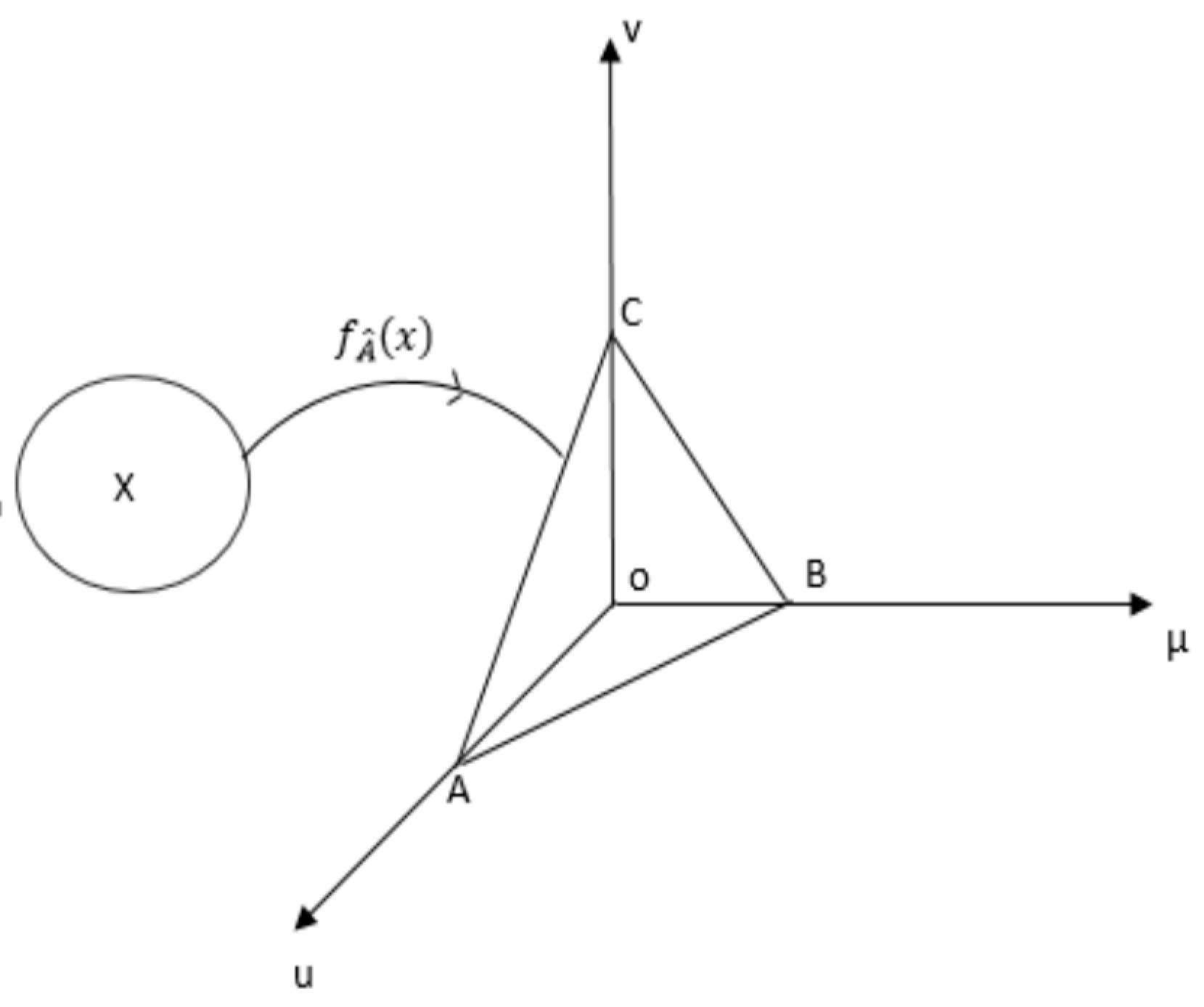
4. Geometrical Interpretation of the Intuitionistic Type-2 Fuzzy Set

Let X be the given universe and $\tilde{A}$ be an IT2FS defined on $X$. Let us construct a mapping $f_{\tilde{A}}\mathrm{from}X\mathrm{to}F$ (a tetrahedron as shown in Figure 1 passing through the points O (0,0,0), A(1,0,0), B(0,1,0), C(0,0,1)) such that for $x\in X$, there exists:

$$y=f_{\tilde{A}}\left(x\right)\in F$$

with the coordinate $\langle u,{\mu }_{\tilde{A}},{\nu }_{\tilde{A}}\rangle$ for which $u\in J_x\subseteq \left[0,1\right]\mathrm{and}0\le {\mu }_{\tilde{A}}+{\nu }_{\tilde{A}}\le 1$.

5. Operations on IT2FS

In this section, similar to several existing set-theoretic operations on fuzzy sets, we also present basic operations such as union, intersection, and complement on the proposed IT2FS.

In this context, let us consider two IT2FS $\tilde{A}$ and $\tilde{B}$ on $X$ as defined below.

$$\tilde{A}={{\displaystyle \int }}_{x\in X}\left({{\displaystyle \int }}_{u\in J_x^u}\left({\mu }_{\tilde{A}}\left(x,u\right), {\nu }_{\tilde{A}}\left(x,u\right)\right)/u\right)/x\mathrm{and} \tilde{B}={{\displaystyle \int }}_{x\in X}\left({{\displaystyle \int }}_{v\in J_x^v}\left({\mu }_{\tilde{B}}\left(x,v\right), {\nu }_{\tilde{B}}\left(x,v\right)\right)/v\right)/x,$$

where $J_x^u\left(\subseteq \left[0,1\right]\right)$ are the domains of the secondary membership function, respectively. Then, the union of $\tilde{A}$ and $\tilde{B}$ is defined as:

$$\tilde{A}\cup \tilde{B}={\int }_{x\in X}\frac{\left({{\displaystyle \int }}_{w\in J_x^w}\frac{\left({\mu }_{\tilde{A}\cup \tilde{B}}\left(x,w\right),{\nu }_{\tilde{A}\cup \tilde{B}}\left(x,w\right)\right)}{w}\right)}{x},J_x^u\cup J_x^v=J_x^w\subseteq \left[0,1\right],$$

where:

$${\mu }_{\tilde{A}\cup \tilde{B}}\left(x\right)=\Phi \left({\int }_{u\in J_x^u}{\mu }_{\tilde{A}}\left(x,u\right),/u,{\int }_{J_x^v}{\mu }_{\tilde{B}}\left(x,v\right),/v\right).$$

By using the extension principle, we obtain,

$${\mu }_{\tilde{A}\cup \tilde{B}}\left(x,w\right)={\int }_{u\in J_x^u}{\int }_{v\in J_x^v}\left({\mu }_{\tilde{A}}\left(x,u\right)\wedge {\mu }_{\tilde{B}}\left(x,v\right)\right)/\Phi \left(u,v\right),$$

where $\Phi \left(u,v\right)$ is the $t$-conorm of $u$ and $v$, i.e.,

$${\mu }_{\tilde{A}\cup \tilde{B}}\left(x,w\right)={\int }_{u\in J_x^u}{\int }_{v\in J_x^v}\left({\mu }_{\tilde{A}}\left(x,u\right)\wedge {\mu }_{\tilde{B}}\left(x,v\right)\right)/\left(u\vee v\right).$$

Similarly,

$${\nu }_{\tilde{A}\cup \tilde{B}}\left(x,w\right)={\int }_{u\in J_x^u}{\int }_{v\in J_x^v}\left({\nu }_{\tilde{A}}\left(x,u\right)\vee {\nu }_{\tilde{B}}\left(x,v\right)\right)/\left(u\vee v\right).$$

The intersection of $\tilde{A}$ and $\tilde{B}$ is defined as:

$$\tilde{A}\cap \tilde{B}={\int }_{x\in X}\left({\int }_{w\in J_x^w}\left({\mu }_{\tilde{A}\cap \tilde{B}}\left(x,w\right),{\nu }_{\tilde{A}\cap \tilde{B}}\left(x,w\right)\right)/w\right)/x,J_x^u\cup J_x^v=J_x^w\subseteq \left[0,1\right],$$

where:

$${\mu }_{\tilde{A}\cap \tilde{B}}\left(x,w\right)={\int }_{u\in J_x^u}{\int }_{v\in J_x^v}\left({\mu }_{\tilde{A}}\left(x,u\right)\wedge {\mu }_{\tilde{B}}\left(x,v\right)\right)/\left(u\wedge v\right)$$

and:

$${\nu }_{\tilde{A}\cup \tilde{B}}\left(x,w\right)={\int }_{u\in J_x^u}{\int }_{v\in J_x^v}\left({\nu }_{\tilde{A}}\left(x,u\right)\vee {\nu }_{\tilde{B}}\left(x,v\right)\right)/\left(u\wedge v\right).$$

The complement of $\tilde{A}$ is defined as:

$${\tilde{A}}^c={\int }_{x\in X}\left({\int }_{u\in J_x^u}\left({\mu }_{\tilde{A}}\left(x\right), {\nu }_{\tilde{A}}\left(x\right)\right)/\left(1-u\right)\right)/x$$

and:

$$\overline{\tilde{A}}={\int }_{x\in X}\left({\int }_{u\in J_x^u}\left({\nu }_{\tilde{A}}\left(x,u\right), {\mu }_{\tilde{A}}\left(x,u\right)\right)/u\right)/x.$$

In addition, there are some more operations on IT2FSs that are defined below.

$$\tilde{A}\subset \tilde{B} iff \left(\forall x\in X\right)\left(u\le v, {\mu }_{\tilde{A}}\left(x,u\right)\le {\mu }_{\tilde{B}}\left(x,v\right) and {\nu }_{\tilde{A}}\left(x,u\right)\ge {\nu }_{\tilde{B}}\left(x,v\right)\right)$$

and:

$$\begin{array}{c}\tilde{A}= \tilde{B} iff \left(\forall x\in X\right)\left(u=v, {\mu }_{\tilde{A}}\left(x,u\right)= {\mu }_{\tilde{B}}\left(x,v\right) and {\nu }_{\tilde{A}}\left(x,u\right)={\nu }_{\tilde{B}}\left(x,v\right)\right)\\ \overline{\tilde{A}}={\displaystyle \sum _{x\in X}}\left({\displaystyle \sum _{u\in J_x}}\left({\nu }_{\tilde{A}}\left(x,u\right),{\mu }_{\tilde{A}}\left(x,u\right)\right)/u\right)/x.\end{array}$$

For the continuous case, ${\displaystyle \sum }$ is replaced by ${\displaystyle \int }$.

We present the following example to illustrate the properties of IT2FS as mentioned below.

Example 4.

Let$\tilde{A}$and$\tilde{B}$be two IT2FSs representing the set young. The youthness is the primary membership function of$\tilde{A}$and$\tilde{B}$. Let the degree of youthness and degree of adultness be the secondary membership and non-membership functions of$\tilde{A}$and$\tilde{B}$, respectively. We consider both$\tilde{A}$and$\tilde{B}$to be defined on$X=\left\{8, 10, 14\right\}$, which are eventually represented as:

$$\begin{array}{cc}\hfill \tilde{A}=(\left(0.9,0.0\right)/0.8& +\left(0.7,0.1\right)/0.9 +\left(0.6,0.3\right)/1.0)/8 + (\left(0.8,0.1\right)/0.6 +\left(0.7,0.2\right)/0.7\hfill \\ \hfill +& \left(0.6,0.4\right)/0.8)/10 +\left(\left(0.9,0.1\right)/0.4 +\left(0.8,0.2\right)/0.5+\left(0.5,0.4\right)/0.6\right)/14\hfill \end{array}$$

and:

$$\begin{array}{cc}\hfill \tilde{B}=(\left(0.8,0.1\right)/0.7& +\left(0.6,0.3\right)/0.8 +\left(0.5,0.5\right)/0.9)/8 + (\left(0.9,0.1\right)/0.4\hfill \\ \hfill +& \left(0.7,0.2\right)/0.5 +\left(0.5,0.3\right)/0.6)/10 +(\left(0.8,0.2\right)/0.5\hfill \\ \hfill +& \left(0.7,0.2\right)/0.6+\left(0.6,0.3\right)/0.7)/14.\hfill \end{array}$$

Now, for a particular element 8the secondary membership and non-membership function of$\tilde{A}$and$\tilde{B}$ are:

$$\left(\left(0.9,0.0\right)/0.8+\left(0.7,0.1\right)/0.9+\left(0.6,0.3\right)/1.0\right)/8$$

and:

$$\left(\left(0.8,0.1\right)/0.7+\left(0.6,0.3\right)/0.8+\left(0.5,0.5\right)/0.9\right)/8$$

respectively.

Then for$x=8$, the union operation of$\tilde{A}$and$\tilde{B}$is$\left({\mu }_{\tilde{A}\cup \tilde{B}}\left(8\right), {\nu }_{\tilde{A}\cup \tilde{B}}\left(8\right)\right)$:

$$\begin{array}{cc}= (\left(0.9,0.0\right)/0.8\hfill & +\left(0.7,0.1\right)/0.9 +\left(0.6,0.3\right)/1.0)/8 \bigvee (\left(0.8,0.1\right)/0.7+\left(0.6,0.3\right)/0.8\hfill \\ & +\left(0.5,0.5\right)/0.9)/8\hfill \\ = (\left(0.9,0.0\right)/0.8\hfill & +\left(0.7,0.1\right)/0.9 +\left(0.6,0.3\right)/1.0)/8 \bigvee (\left(0.8,0.1\right)/0.7+\left(0.6,0.3\right)/0.8\hfill \\ & +\left(0.5,0.5\right)/0.9)/8\hfill \\ =((\left(0.9\wedge 0.8\right),(\hfill & 0.0\vee 0.1\left)\right)/\left(0.8\vee 0.7\right) +\left(\left(0.7\wedge 0.8\right),\left(0.1\vee 0.1\right)\right)/\left(0.9\vee 0.7\right)+ ((0.6\hfill \\ & \wedge 0.8),\left(0.3\vee 0.1\right) )/\left(1.0\vee 0.7\right)+\left(\left(0.9\wedge 0.6\right),\left(0.0\vee 0.3\right)\right)/\left(0.8\vee 0.8\right)\hfill \\ & + \left(\left(0.7\wedge 0.6\right),\left(0.1\vee 0.3\right) \right)/\left(0.9\vee 0.8\right)+\left(\left(0.6\wedge 0.6\right),\left(0.3\vee 0.3\right) \right)/(1.0\hfill \\ & \vee 0.8)+ \left(\left(0.9\wedge 0.5\right),\left(0.0\vee 0.5\right) \right)/\left(0.8\vee 0.9\right)+ (\left(0.7\wedge 0.5\right),(0.1\hfill \\ & \vee 0.5) )/\left(0.9\vee 0.9\right)+ \left(\left(0.6\wedge 0.5\right),\left(0.3\vee 0.5\right) \right)/\left(0.1\vee 0.9\right))/8\hfill \\ =(\left(0.8,0.1\right)/0.8\hfill & +\left(0.7,0.1\right)/0.9 +\left(0.6,0.3\right)/1.0 +\left( 0.6,0.3\right)/0.8 +\left(0.6,0.3\right)/0.9\hfill \\ & +\left(0.6,0.3\right)/1.0 +\left(0.5,0.5\right)/0.9 +\left(0.5,0.5\right)/0.9+\left(0.5,0.5\right)/1.0)/8\hfill \\ =((max\left\{0.8,0.6\right\}\hfill & ,min\left\{0.1,0.3\right\})/0.8 +\left(max\left\{0.7,0.6,0.5,0.5\right\}, min\left\{0.1,0.3,0.5,0.5\right\}\right)/0.9\hfill \\ & +\left(max\left\{0.6,0.6,0.5\right\}, min\left\{0.3,0.3,0.5\right\}/1.0 \right)/8\hfill \\ =(\left(0.8,0.1\right)/0.8\hfill & +\left(0.7,0.1\right)/0.9 +\left(0.6,0.3\right)/1.0)/8.\hfill \end{array}$$

Similarly, the intersection is given by$\left({\mu }_{\tilde{A}\cap \tilde{B}}\left(8\right), {\nu }_{\tilde{A}\cap \tilde{B}}\left(8\right)\right)$:

$$\begin{array}{cc}=(\left(0.9,0.0\right)/0.8\hfill & +\left(0.7,0.1\right)/0.9+\left(0.6,0.3\right)/1.0)/8\wedge (\left(0.8,0.1\right)/0.7+\left(0.6,0.3\right)/0.8\hfill \\ & +\left(0.5,0.5\right)/0.9)/8\hfill \\ = ((\left(0.9\wedge 0.8\right),\hfill & \left(0.0\vee 0.1\right))/\left(0.8\wedge 0.7\right)+\left(\left(0.7\wedge 0.8\right),\left(0.1\vee 0.1\right)\right)/\left(0.9\wedge 0.7\right)+ ((0.6\hfill \\ & \wedge 0.8),\left(0.3\vee 0.1\right) )/\left(1.0\wedge 0.7\right)+\left(\left(0.9\wedge 0.6\right),\left(0.0\vee 0.3\right) \right)/\left(0.8\wedge 0.8\right)\hfill \\ & + \left(\left(0.7\wedge 0.6\right),\left(0.1\vee 0.3\right) \right)/\left(0.9\wedge 0.8\right)+\left(\left(0.6\wedge 0.6\right),\left(0.3\vee 0.3\right) \right)/(1.0\hfill \\ & \wedge 0.8)+ \left(\left(0.9\wedge 0.5\right),\left(0.0\vee 0.5\right) \right)/\left(0.8\wedge 0.9\right)+(\left(0.7\wedge 0.5\right),(0.1\hfill \\ & \vee 0.5) )/\left(0.9\wedge 0.9\right)+ \left(\left(0.6\wedge 0.5\right),\left(0.3\vee 0.5\right) \right)/\left(0.1\wedge 0.9\right))/8.\hfill \\ =(\left(0.8,0.1\right)/0.7\hfill & +\left(0.7,0.1\right)/0.7 +\left(0.6,0.3\right)/0.7+ \left( 0.6,0.3\right)/0.8+\left(0.6,0.3\right)/0.8\hfill \\ & +\left(0.6,0.3\right)/0.8+\left(0.5,0.5\right)/0.8 +\left(0.5,0.5\right)/0.9+\left(0.5,0.5\right)/0.9)/8\hfill \\ =((max\{0.8,0.7,\hfill & 0.6\}, min\left\{0.1,0.1,0.3\right\})/0.7\hfill \\ & +\left(max\left\{0.6,0.6,0.6,0.5\right\}, min\left\{0.3,0.3,0.3,0.5\right\}\right)/0.8\hfill \\ & +\left(max\left\{0.5,0.5\right\}, min\left\{0.5,0.5\right\}/0.9\right)/8\hfill \\ =(\left(0.8,0.1\right)/0.7\hfill & +\left(0.6,0.3\right)/0.8 +\left(0.5,0.5\right)/0.9)/8\hfill \end{array}$$

$$\begin{array}{cc}\hfill {\tilde{A}}^c=(\left(0.9,0.0\right)/& 0.2 +\left(0.7,0.1\right)/0.1 +\left(0.3,0.6\right)/0.0)/8 + (\left(0.8,0.1\right)/0.4 +\left(0.7,0.2\right)/0.3\hfill \\ & +\left(0.6,0.4\right)/0.2)/10 +\left(\left(0.9,0.1\right)/0.6 +\left(0.8,0.2\right)/0.5+\left(0.5,0.4\right)/0.4\right)/14\hfill \end{array}$$

and:

$$\begin{array}{cc}\hfill \overline{\tilde{A}}=(\left(0.0,0.9\right)/0.8& +\left(0.1,0.7\right)/0.9 +\left(0.3,0.6\right)/1.0)/8 +(\left(0.1,0.8\right)/0.6 +\left(0.2,0.7\right)/0.7\hfill \\ \hfill +& \left(0.4,0.6\right)/0.8)/10 +\left(\left(0.1,0.9\right)/0.4 +\left(0.2,0.8\right)/0.5+\left(0.4,0.5\right)/0.6\right)/14.\hfill \end{array}$$

6. Properties of IT2FS

Considering various set-theoretic properties like $idempotency,commutativity$, $associativity$, $distributivelaw$, $involution$, and $DeMorgan’slaw$, which exist for a fuzzy set and an intuitionistic fuzzy set. In this section, analogously, we also define similar properties for IT2FS along with necessary and relevant examples. Subsequently, we consider three IT2FSs $\tilde{A},\tilde{B},$ and $\tilde{C},$ and we define these operations as presented below.

(i)

$\tilde{A} \cup \tilde{A}=\tilde{A} (Idempotency)$

(ii)

$\tilde{A}\cup \tilde{B}=\tilde{B} \cup \tilde{A}, \tilde{A} \cap \tilde{B}=\tilde{B}\cap \tilde{A} (Commutativity)$

(iii)

$(\tilde{A}\cup \tilde{B})\cup \tilde{C} =\tilde{A} \cup (\tilde{B}\cup \tilde{C}), (\tilde{A}\cap \tilde{B})\cap \tilde{C} =\tilde{A} \cap (\tilde{B}\cap \tilde{C}) (Associativity)$

(iv)

$\tilde{A} \cup (\tilde{B}\cap \tilde{C})=(\tilde{A}\cup \tilde{B})\cap (\tilde{A}\cup \tilde{C}), \tilde{A} \cap (\tilde{B}\cup \tilde{C}) =(\tilde{A}\cap \tilde{B})\cup (\tilde{A}\cap \tilde{C}) (Distributive law)$

(v)

${({\tilde{A}}^c)}^c =\tilde{A} (Involution)$

(vi)

${(\tilde{A}\cup \tilde{B})}^C={\tilde{A}}^c\cap {\tilde{B}}^c, {(\tilde{A}\cup \tilde{B})}^C={\tilde{A}}^c\cup {\tilde{B}}^c (De Morga{n}^{’}s law)$

The proofs of (i)–(iii) and (v) are obvious. We illustrate these results later by examples.

Proof of (vi).

$$\begin{array}{l}{(\tilde{A}\cup \tilde{B})}^C\\ ={\left\{\langle x,\left(u\vee v\right), {\mu }_{\tilde{A}}\left(x,u\right)\wedge {\mu }_{\tilde{B}}\left(x,v\right),{\nu }_{\tilde{A}}\left(x,u\right)\wedge {\nu }_{\tilde{B}}\left(x,v\right)\rangle /x\in X,u,v\in J_{\mathrm{x}}\subseteq \left[0,1\right]\right\}}^c\\ =\left\{\langle x,\left(1-u\vee v\right), {\mu }_{\tilde{A}}\left(x,u\right)\wedge {\mu }_{\tilde{B}}\left(x,v\right),{\nu }_{\tilde{A}}\left(x,u\right)\wedge {\nu }_{\tilde{B}}\left(x,v\right)\rangle /x\in X,u,v\in J_{\mathrm{x}}\subseteq \left[0,1\right]\right\}\\ =\langle \left\{x,\left(1-u\vee 1-v\right), {\mu }_{\tilde{A}}\left(x,u\right)\wedge {\mu }_{\tilde{B}}\left(x,v\right),{\nu }_{\tilde{A}}\left(x,u\right)\wedge {\nu }_{\tilde{B}}\left(x,v\right)\rangle /x\in X,u,v\in J_{\mathrm{x}}\subseteq \left[0,1\right]\right\}\\ =\langle \left\{x,\left(1-u\right), {\mu }_{\tilde{A}}\left(x,u\right),{\nu }_{\tilde{A}}\left(x,u\right)\rangle /x\in X,u\in J_{\mathrm{x}}\subseteq \left[0,1\right]\right\}\\ \cap \left\{\langle x,\left(1-v\right), {\mu }_{\tilde{B}}\left(x,v\right),{\nu }_{\tilde{B}}\left(x,v\right)\rangle /x\in X,v\in J_{\mathrm{x}}\subseteq \left[0,1\right]\right\}\\ = {\tilde{A}}^c\cap {\tilde{B}}^c.\end{array}$$

Furthermore:

$$\begin{array}{l}{(\tilde{A}\cup \tilde{B})}^C\\ ={\left\{\langle x,\left(u\wedge v\right), {\mu }_{\tilde{A}}\left(x,u\right)\wedge {\mu }_{\tilde{B}}\left(x,v\right),{\nu }_{\tilde{A}}\left(x,u\right)\vee {\nu }_{\tilde{B}}\left(x,v\right)\rangle /x\in X,u,v\in J_{\mathrm{x}}\subseteq \left[0,1\right]\right\}}^c\\ =\left\{\langle x,\left(1-u\wedge v\right), {\mu }_{\tilde{A}}\left(x,u\right)\wedge {\mu }_{\tilde{B}}\left(x,v\right),{\nu }_{\tilde{A}}\left(x,u\right)\vee {\nu }_{\tilde{B}}\left(x,v\right)\rangle /x\in X,u,v\in J_{\mathrm{x}}\subseteq \left[0,1\right]\right\}\\ =\left\{\langle x,\left(1-u\vee 1-v\right), {\mu }_{\tilde{A}}\left(x,u\right)\wedge {\mu }_{\tilde{B}}\left(x,v\right),{\nu }_{\tilde{A}}\left(x,u\right)\vee {\nu }_{\tilde{B}}\left(x,v\right)\rangle /x\in X,u,v\in J_{\mathrm{x}}\subseteq \left[0,1\right]\right\}\\ =\left\{\langle x,\left(1-u\right), {\mu }_{\tilde{A}}\left(x,u\right),{\nu }_{\tilde{A}}\left(x,u\right)\rangle /x\in X,u\in J_{\mathrm{x}}\subseteq \left[0,1\right]\right\}\\ \cup \left\{\langle x,\left(1-v\right), {\mu }_{\tilde{B}}\left(x,v\right),{\nu }_{\tilde{B}}\left(x,v\right)\rangle /x\in X,v\in J_{\mathrm{x}}\subseteq \left[0,1\right]\right\}\\ ={\tilde{A}}^c\cup {\tilde{B}}^c.\end{array}$$

 □

Example 5.

Let$\tilde{A},\tilde{B}, \tilde{C}$be the three IT2FS on$X=\left\{6, 5, 4\right\}$defined as:

$$\tilde{A}=\left(1.0,0.0\right)/0.9/6 + \left(0.1,0.7\right)/0.3/5 + \left(0.4,0.5\right)/0.6/4$$

$$\tilde{B}=\left(0.8,1.0\right)/0.4/6 + \left(0.1,0.8\right)/0.5/5 + \left(0.5,0.5\right)/0.9/4$$

and:

$$\tilde{C}=\left(0.1,0.8\right)/0.0/6 + \left(1.0,0.0\right)/0.9/5 + \left(0.4,0.4\right)/0.7/4.$$

For simplicity, we have taken$J_x$as a singleton set for each$x\in X$.

Then:

$$\tilde{A}\cup \tilde{A}=\left(1.0,0.0\right)/0.9/6 + \left(0.1,0.7\right)/0.3/5 + \left(0.4,0.5\right)/0.6/4 =\tilde{A}.$$

Therefore, the idempotent property holds.

$$\tilde{A}\cup \tilde{B}=\left(0.8,1.0\right)/0.9/6 + \left(0.1,0.8\right)/0.5/5 + \left(0.4,0.5\right)/0.9/4$$

and:

$$\tilde{B}\cup \tilde{A}=\left(0.8,1.0\right)/0.9/6 + \left(0.1,0.8\right)/0.5/5 + \left(0.4,0.5\right)/0.9/4.$$

Correspondingly,

$$\tilde{A}\cap \tilde{B}=\left(0.8,1.0\right)/0.4/6 + \left(0.1,0.8\right)/0.3/5 + \left(0.4,0.5\right)/0.6/4$$

and:

$$\tilde{B}\cap \tilde{A}=\left(0.8,1.0\right)/0.4/6 + \left(0.1,0.8\right)/0.3/5 + \left(0.4,0.5\right)/0.6/4.$$

Therefore, the commutative property holds.

$$(\tilde{A}\cup \tilde{B})\cup \tilde{C}=(0.1,0.8)/0.9/6 + (0.1,0.8)/0.9/5 + (0.4,0.5)/0.9/4$$

and:

$$\tilde{A} \cup (\tilde{B}\cup \tilde{C})=(0.1,0.8)/0.9/6 + (0.1,0.8)/0.9/5 + (0.4,0.5)/0.9/4.$$

Likewise,

$$(\tilde{A}\cap \tilde{B})\cap \tilde{C}=(0.1,0.8)/0.0/6 + (0.1,0.8)/0.3/5 + (0.4,0.5)/0.6/4$$

and:

$$\tilde{A} \cap (\tilde{B}\cap \tilde{C})=(0.1,0.8)/0.0/6 + (0.1,0.8)/0.3/5 + (0.4,0.5)/0.6/4.$$

Therefore, the associative property holds.

$$\tilde{A} \cup (\tilde{B}\cap \tilde{C})=(0.1,0.8)/0.9/6 + (0.1,0.8)/0.5/5 + (0.4,0.5)/0.7/4$$

and:

$$(\tilde{A}\cup \tilde{B})\cap (\tilde{A}\cup \tilde{C})=(0.1,0.8)/0.9/6 + (0.1,0.8)/0.5/5 + (0.4,0.5)/0.7/4.$$

Moreover,

$$\tilde{A} \cap (\tilde{B}\cup \tilde{C})=(0.1,0.8)/0.4/6 + (0.1,0.8)/0.3/5 + (0.4,0.5)/0.6/4$$

and:

$$(\tilde{A}\cap \tilde{B})\cup (\tilde{A}\cap \tilde{C})=(0.1,0.8)/0.4/6 + (0.1,0.8)/0.3/5 + (0.4,0.5)/0.6/4.$$

Therefore, the distributive property holds.

$${({\tilde{A}}^c)}^c =(1.0,0.0)/0.9/6 + (0.1,0.7)/0.3/5 + (0.4,0.5)/0.6/4 =\tilde{A}.$$

Therefore, the involution property holds.

$${(\tilde{A}\cap \tilde{B})}^c=(0.8,1.0)/0.6/6 + (0.1,0.8)/0.7/5 + (0.4,0.5)/0.4/4$$

and:

$${\tilde{A}}^C\cup {\tilde{B}}^C=(0.8,1.0)/0.6/6 + (0.1,0.8)/0.7/5 + (0.4,0.5)/0.4/4.$$

Furthermore,

$${(\tilde{A}\cup \tilde{B})}^c=(0.8,1.0)/0.1/6 + (0.1,0.8)/0.5/5 + (0.4,0.5)/0.1/4$$

and:

$${\tilde{A}}^C\cap {\tilde{B}}^C=(0.8,1.0)/0.1/6 + (0.1,0.8)/0.5/5 + (0.4,0.5)/0.1/4.$$

Therefore, De Morgan’s law holds.

7. Necessity and Possibility Operators on IT2FS

Keeping in view the existence of several measure functions of the fuzzy set and its variants, in this section, we propose the possibility and necessity of IT2FS. There are some cases in which we need a gross result. From an IT2FS, if we want a gross result in terms of ordinary T2FS, then we need two operators that can transform an IT2FS into an ordinary T2FS. Let $\tilde{A}$ be an IT2FS over $X$ with primary membership function $u$, secondary membership function ${\mu }_{\tilde{A}}\left(x,u\right)$, and secondary non-membership function ${\nu }_{\tilde{A}}\left(x,u\right)$. Then, the two operators are defined as follows.

(i)

Necessity operator:

$$\Delta \tilde{A}=\left\{\langle x,u,{\mu }_{\tilde{A}}\left(x,u\right),1-{\mu }_{\tilde{A}}\left(x,u\right)\rangle :\mathrm{x}\in \mathrm{X},\mathrm{u}\in J_{\mathrm{x}}\subseteq \left[0,1\right]\right\}.$$

(ii)

Possibility operator:

$$\nabla \tilde{A}=\left\{\langle x,u,1-{\nu }_{\tilde{A}}\left(x,u\right),{\nu }_{\tilde{A}}\left(x,u\right)\rangle :\mathrm{x}\in \mathrm{X},\mathrm{u}\in J_{\mathrm{x}}\subseteq \left[0,1\right]\right\}.$$

The operators can also be represented as:

$$\Delta \tilde{A}={\int }_{x\in X}\left({\int }_{u\in J_x}{\mu }_{\tilde{A}}\left(x,u\right), 1-{\mu }_{\tilde{A}}\left(x,u\right)\right)/u)/x$$

and:

$$\nabla \tilde{A}={\int }_{x\in X}\left({\int }_{u\in J_x}{\mu }_{\tilde{A}}\left(x,u\right), {\nu }_{\tilde{A}}\left(x,u\right)\right)/u)/x.$$

For the discrete case, ${\displaystyle \sum }$ is replaced by ${\displaystyle \int }$.

Obviously, if $\tilde{A}$ is an ordinary T2FS, then $\Delta \tilde{A}=\tilde{A}=\nabla \tilde{A}$. Let us now explain this idea by an example.

Example 6.

Consider Example 3 in Section 3.

$$\begin{array}{cc}\hfill \tilde{A}=(\left(0.9,0.0\right)/0.8& +\left(0.7,0.1\right)/0.9+\left(0.6,0.3\right)/1.0)/8+(\left(0.8,0.1\right)/0.6 +\left(0.7,0.2\right)/0.7\hfill \\ \hfill +& \left(0.6,0.4\right)/0.8)/10+\left(0.9,0.1\right)/0.4 +\left(0.8,0.2\right)/0.5+\left(0.5,0.5\right)/0.6)/14.\hfill \end{array}$$

Now, for this set $\tilde{A}$:

$$\begin{array}{cc}\hfill \Delta \tilde{A}=(\left(0.9,0.1\right)/& 0.8 +\left(0.7,0.3\right)/0.9 +\left(0.6,0.4\right)/1.0)/8 + (\left(0.8,0.2\right)/0.6 +\left(0.7,0.3\right)/0.7\hfill \\ & +\left(0.6,0.4\right)/0.8)/10 +\left(\left(0.9,0.1\right)/0.4 +\left(0.8,0.2\right)/0.5+\left(0.5,0.5\right)/0.6\right)/14.\hfill \end{array}$$

and:

$$\begin{array}{cc}\hfill \nabla \tilde{A}=(\left(1.0,0.0\right)/& 0.8 +\left(0.9,0.1\right)/0.9 +\left(0.7,0.3\right)/1.0)/8 + (\left(0.9,0.1\right)/0.6 +\left(0.8,0.2\right)/0.7\hfill \\ & +\left(0.6,0.4\right)/0.8)/10 +\left(\left(0.9,0.1\right)/0.4 +\left(0.8,0.2\right)/0.5+\left(0.6,0.4\right)/0.6\right)/14.\hfill \end{array}$$

Proposition

Here, we compile some relevant properties of the necessity and possibility operators of IT2FS. For every IT2FS $\tilde{A}$, we have:

(i)

$\overline{\Delta \overline{\tilde{A}}}= \nabla \tilde{A}$

(ii)

$\overline{\nabla \overline{\tilde{A}}}= \Delta \tilde{A}$

(iii)

$\Delta \Delta \tilde{A}= \Delta \tilde{A}$

(iv)

$\Delta \nabla \tilde{A}= \nabla \tilde{A}$

(v)

$\nabla \Delta \tilde{A}= \Delta \tilde{A}$

(vi)

$\nabla \nabla \tilde{A}= \nabla \tilde{A}$

(vii)

$\Delta \tilde{A}\subset \tilde{A}\subset \nabla \tilde{A}$

Proof. 

(i)

$\begin{array}{l}\overline{\Delta \overline{\tilde{A}}}= \overline{\Delta \langle \{x,u,{\nu }_{\tilde{A}}(x,u),{\mu }_{\tilde{A}}(x,u)\rangle /x:\mathrm{x}\in \mathrm{X},\mathrm{u}\in J_{\mathrm{x}}\subseteq \left[0,1\right]\}}=\\ \overline{\{\langle x,u,{\nu }_{\tilde{A}}(x,u),1-{\nu }_{\tilde{A}}(x,u)\rangle /x:\mathrm{x}\in \mathrm{X},\mathrm{u}\in J_{\mathrm{x}}\subseteq \left[0,1\right]\}}= \{\langle x,u,1-{\nu }_{\tilde{A}}(x,u),{\nu }_{\tilde{A}}(x,u)\rangle /x:\mathrm{x}\in \mathrm{X},\mathrm{u}\in \\ J_{\mathrm{x}}\subseteq \left[0,1\right]\}= \nabla \tilde{A}.\end{array}$

(ii)

$\begin{array}{l}\overline{\nabla \overline{\tilde{A}}}= \overline{\nabla \{\langle x,u,{\nu }_{\tilde{A}}(x,u),{\mu }_{\tilde{A}}(x,u)\rangle /x:\mathrm{x}\in \mathrm{X},\mathrm{u}\in J_{\mathrm{x}}\subseteq \left[0,1\right]\}}=\\ \overline{\{\langle x,u,1-{\mu }_{\tilde{A}}(x,u),{\mu }_{\tilde{A}}(x,u)\rangle /x:\mathrm{x}\in \mathrm{X},\mathrm{u}\in J_{\mathrm{x}}\subseteq \left[0,1\right]\}}= \{\langle x,u,{\mu }_{\tilde{A}}(x,u),1-{\mu }_{\tilde{A}}(x,u)\rangle /x:\mathrm{x}\in \\ \mathrm{X},\mathrm{u}\in J_{\mathrm{x}}\subseteq \left[0,1\right]\}= \Delta \tilde{A}.\end{array}$

(iii)

$\begin{array}{l}\Delta \Delta \tilde{A}=\Delta \{\langle x,u,{\mu }_{\tilde{A}}(x,u),1-{\mu }_{\tilde{A}}(x,u)\rangle /x:\mathrm{x}\in \mathrm{X},\mathrm{u}\in J_{\mathrm{x}}\subseteq \left[0,1\right]\}=\{\langle x,u,{\mu }_{\tilde{A}}(x,u),1-{\mu }_{\tilde{A}}(x,u)\rangle /\\ x:\mathrm{x}\in \mathrm{X},\mathrm{u}\in J_{\mathrm{x}}\subseteq \left[0,1\right]\}= \Delta \tilde{A}.\end{array}$

(iv)

$\begin{array}{l}\Delta \nabla \tilde{A}=\Delta \{\langle x,u,1-{\nu }_{\tilde{A}}(x,u),{\nu }_{\tilde{A}}(x,u)\rangle /x:\mathrm{x}\in \mathrm{X},\mathrm{u}\in J_{\mathrm{x}}\subseteq \left[0,1\right]\}=\{\langle x,u,1-{\nu }_{\tilde{A}}(x,u),1-(1-\\ {\nu }_{\tilde{A}}(x,u))\rangle /x:\mathrm{x}\in \mathrm{X},\mathrm{u}\in J_{\mathrm{x}}\subseteq \left[0,1\right]\}=\{\langle x,u,1-{\nu }_{\tilde{A}}(x,u),{\nu }_{\tilde{A}}(x,u)\rangle /x:\mathrm{x}\in \mathrm{X},\mathrm{u}\in J_{\mathrm{x}}\subseteq \left[0,1\right]\}= \nabla \tilde{A}.\end{array}$

(v)

$\begin{array}{l}\nabla \Delta \tilde{A}=\nabla \{\langle x,u,{\mu }_{\tilde{A}}(x,u),1-{\mu }_{\tilde{A}}(x,u)\rangle /x:\mathrm{x}\in \mathrm{X},\mathrm{u}\in J_{\mathrm{x}}\subseteq \left[0,1\right]\}=\{\langle x,u,1-(1-{\mu }_{\tilde{A}}(x,u),(1-\\ {\mu }_{\tilde{A}}(x,u))\rangle /x:\mathrm{x}\in \mathrm{X},\mathrm{u}\in J_{\mathrm{x}}\subseteq \left[0,1\right]\}=\{\langle x,u,{\mu }_{\tilde{A}}(x,u),1-{\mu }_{\tilde{A}}(x,u)\rangle /x:\mathrm{x}\in \mathrm{X},\mathrm{u}\in J_{\mathrm{x}}\subseteq \left[0,1\right]\}= \Delta \tilde{A}.\end{array}$

(vi)

$\begin{array}{l}\nabla \nabla \tilde{A}=\nabla \{\langle x,u,1-{\nu }_{\tilde{A}}(x,u),{\nu }_{\tilde{A}}(x,u)\rangle /x:\mathrm{x}\in \mathrm{X},\mathrm{u}\in J_{\mathrm{x}}\subseteq \left[0,1\right]\}=\{\langle x,u,1-{\nu }_{\tilde{A}}(x,u),{\nu }_{\tilde{A}}(x,u))\rangle /\\ x:\mathrm{x}\in \mathrm{X},\mathrm{u}\in J_{\mathrm{x}}\subseteq \left[0,1\right]\}= \nabla \tilde{A}.\end{array}$

(vii)

$\Delta \tilde{A}=\{\langle x,u,{\mu }_{\tilde{A}}(x,u),1-{\mu }_{\tilde{A}}(x,u)\rangle /x:\mathrm{x}\in \mathrm{X},\mathrm{u}\in J_{\mathrm{x}}\subseteq \left[0,1\right]\}.$

Now, $1-{\mu }_{\widetilde{A }}(x,u)\ge {\nu }_{\widetilde{A }}(x,u)\left[since 0\le {\mu }_{\tilde{A}}(x,u)+ {\nu }_{\tilde{A}}(x,u)\le 1\right]$.

Therefore,

$$\begin{array}{cc}\hfill \{\langle x,u,{\mu }_{\tilde{A}}(x,u),1& -{\mu }_{\tilde{A}}(x,u)\rangle /x:\mathrm{x}\in \mathrm{X},\mathrm{u}\in J_{\mathrm{x}}\subseteq \left[0,1\right]\}\hfill \\ & \subset \{\langle x,u,{\mu }_{\tilde{A}}(x,u),{\nu }_{\tilde{A}}(x,u)\rangle /x:\mathrm{x}\in \mathrm{X},\mathrm{u}\in J_{\mathrm{x}}\subseteq \left[0,1\right]\}.\hfill \end{array}$$

Hence, $\tilde{A}\subset \nabla \tilde{A}$.

$$\mathrm{Consequently},\mathrm{both}\mathrm{imply} \Delta \tilde{A}\subset \tilde{A}\subset \nabla \tilde{A}$$

 □

Theorem 1.

For any two IT2FSs$\tilde{A}$and $\tilde{B}$, we have:

(i)

$\Delta (\tilde{A}\cap \tilde{B})= \Delta \tilde{A}\cap \Delta \tilde{B}$

(ii)

$\Delta (\tilde{A}\cup \tilde{B})= \Delta \tilde{A} \cup \Delta \tilde{B}$

(iii)

$\nabla (\tilde{A}\cap \tilde{B})= \nabla \tilde{A} \cap \nabla \tilde{B}$

(iv)

$\nabla (\tilde{A}\cup \tilde{B})= \nabla \tilde{A} \cup \nabla \tilde{B}$

Proof. 

(i)

$\begin{array}{l}\Delta (\tilde{A}\cap \tilde{B})=\Delta \{\langle x,u\wedge v, {\mu }_{\tilde{A}}(x,u)\wedge {\mu }_{\tilde{B}}(x,v),{\nu }_{\tilde{A}}(x,u)\vee {\nu }_{\tilde{B}}(x,v)\rangle /x\in X,u,v\in J_{\mathrm{x}}\subseteq \left[0,1\right]\}=\\ \{\langle x,(u\wedge v), {\mu }_{\tilde{A}}(x,u)\wedge {\mu }_{\tilde{B}}(x,v), 1- (({\mu }_{\widetilde{A }}(x,u)\bigvee {\mu }_{\tilde{B}}(x,v))\rangle /x\in X,u,v\in J_{\mathrm{x}}\subseteq \left[0,1\right]\}=\{\langle x,(u\wedge \\ v), {\mu }_{\tilde{A}}(x,u)\wedge {\mu }_{\tilde{B}}(x,v), (1-{\mu }_{\widetilde{A }}(x,u))\vee (1-{\mu }_{\tilde{B}}(x,v))\rangle /x\in X,u,v\in J_{\mathrm{x}}\subseteq \left[0,1\right]\}=\\ \{\langle x,u, {\mu }_{\tilde{A}}(x,u), (1-{\mu }_{\widetilde{A }}(x,u))\rangle /x\in X,u,v\in J_{\mathrm{x}}\subseteq \left[0,1\right]\}\cap \{\langle x,v, {\mu }_{\tilde{B}}(x,v), (1-{\mu }_{\tilde{B}}(x,v))\rangle /x\in \\ X,u,v\in J_{\mathrm{x}}\subseteq \left[0,1\right]\}=\Delta \tilde{A} \cap \Delta \tilde{B}\end{array}$

(ii)

$\begin{array}{l}\Delta (\tilde{A}\cup \tilde{B})=\Delta \{\langle x,u\bigvee v, {\mu }_{\tilde{A}}(x,u)\wedge {\mu }_{\tilde{B}}(x,v),{\nu }_{\tilde{A}}(x,u)\vee {\nu }_{\tilde{B}}(x,v)\rangle /x\in X,u,v\in J_{\mathrm{x}}\subseteq \left[0,1\right]\}=\\ \{\langle x,(u\bigvee v), {\mu }_{\tilde{A}}(x,u)\wedge {\mu }_{\tilde{B}}(x,v), 1- (({\mu }_{\widetilde{A }}(x,u)\bigvee {\mu }_{\tilde{B}}(x,v))\rangle /x\in X,u,v\in J_{\mathrm{x}}\subseteq \left[0,1\right]\}=\\ \{\langle x,(u\bigvee v), {\mu }_{\tilde{A}}(x,u)\wedge {\mu }_{\tilde{B}}(x,v), (1-{\mu }_{\widetilde{A }}(x,u))\vee (1-{\mu }_{\tilde{B}}(x,v)) \rangle /x\in X,u,v\in J_{\mathrm{x}}\subseteq \left[0,1\right]\}=\\ \{\langle x,u, {\mu }_{\tilde{A}}(x,u), (1-{\mu }_{\widetilde{A }}(x,u))\rangle /x\in X,u,v\in J_{\mathrm{x}}\subseteq \left[0,1\right]\}\cap \{\langle x,v, {\mu }_{\tilde{B}}(x,v), (1-{\mu }_{\tilde{B}}(x,v))\rangle /x\in \\ X,u,v\in J_{\mathrm{x}}\subseteq \left[0,1\right]\}=\Delta \tilde{A}\cup \Delta \tilde{B}\end{array}$.

(iii)

$\begin{array}{l}\nabla (\tilde{A}\cap \tilde{B})=\nabla \{\langle x,u\wedge v, {\mu }_{\tilde{A}}(x,u)\wedge {\mu }_{\tilde{B}}(x,v),{\nu }_{\tilde{A}}(x,u)\vee {\nu }_{\widetilde{B }}(x,v)\rangle /x\in X,u,v\in J_{\mathrm{x}}\subseteq \left[0,1\right]\}=\\ \{\langle x,u\wedge v,1- (v_{\tilde{A}}(x,u)\bigvee {\mu }_{\tilde{B}}(x,v)), ({\nu }_{\tilde{A}}(x,u)\bigvee {\nu }_{\widetilde{B }}(x,v)\rangle /x\in X,u,v\in J_{\mathrm{x}}\subseteq \left[0,1\right]\}=\{x,u\wedge v,(1-\\ {\nu }_{\widetilde{A }}(x,u)\wedge 1-{\nu }_{\tilde{B}}(x,v)), {\nu }_{\tilde{A}}(x,u)\vee {\nu }_{\tilde{B}}(x,v)\rangle /x\in X,u,v\in J_{\mathrm{x}}\subseteq \left[0,1\right]\}=\{x,u, 1-\\ {\nu }_{\tilde{A}}(x,u), {\nu }_{\tilde{A}}(x,u)\rangle /x\in X,u,v\in J_{\mathrm{x}}\subseteq \left[0,1\right]\}\cap \{x,u, 1-{\nu }_{\tilde{B}}(x,u), {\nu }_{\tilde{B}}(x,u)\rangle /x\in X,u,v\in J_{\mathrm{x}}\subseteq \\ \left[0,1\right]\}=\nabla \tilde{A}\cap \nabla \tilde{B}.\end{array}$

(iv)

$\begin{array}{l}\nabla (\tilde{A}\cup \tilde{B})=\nabla \{\langle x,u\bigvee v, {\mu }_{\tilde{A}}(x,u)\wedge {\mu }_{\tilde{B}}(x,v),{\nu }_{\tilde{A}}(x,u)\vee {\nu }_{\tilde{B}}(x,v)\rangle /x\in X,u,v\in J_{\mathrm{x}}\subseteq \left[0,1\right]\}=\\ \{\langle x,u\bigvee v,(1- {\nu }_{\widetilde{A }}(x,u))\bigvee {\nu }_{\tilde{B}}(x,v), ({\nu }_{\tilde{A}}(x,u)\bigvee {\nu }_{\tilde{B}}(x,v)/x\in X,u,v\in J_{\mathrm{x}}\subseteq \left[0,1\right]\}=\{x,u\bigvee v,(1-\\ {\nu }_{\widetilde{A }}(x,u))\wedge (1-{\nu }_{\tilde{B}}(x,v)), {\nu }_{\tilde{A}}(x,u)\vee {\nu }_{\tilde{B}}(x,v)\rangle /x\in X,u,v\in J_{\mathrm{x}}\subseteq \left[0,1\right]\}=\{x,u, 1-\\ {\nu }_{\tilde{A}}(x,u), {\nu }_{\tilde{A}}(x,u)\rangle /x\in X,u,v\in J_{\mathrm{x}}\subseteq \left[0,1\right]\}\bigcup \{\frac{\langle x,u, 1-{\nu }_{\tilde{B}}(x,u), {\nu }_{\tilde{B}}(x,u)\rangle }{x}\in X,u,v\in J_{\mathrm{x}}\subseteq \left[0,1\right]\}=\nabla \tilde{A}\bigcup \nabla \tilde{B}.\end{array}$

By virtue of the above results, we can define the following relations. □

Definition 1.

For any two IT2FSs$\tilde{A}$and$\tilde{B}$, we define the following relations.

$$\left[\tilde{\mathrm{A}}{\subset }_{\Delta }\tilde{\mathrm{B}}\mathrm{iff}\left(\forall \mathrm{x}\in \mathrm{X}\right)\mathrm{u}\le \mathrm{v},{\mathsf{\mu }}_{\tilde{\mathrm{A}}}\left(\mathrm{x},\mathrm{u}\right)\le {\mathsf{\mu }}_{\tilde{\mathrm{B}}}\left(\mathrm{x},\mathrm{v}\right)\right]\left[\tilde{\mathrm{A}}{\subset }_{\nabla }\tilde{\mathrm{B}}\mathrm{iff}\left(\forall \mathrm{x}\in \mathrm{X}\right)\left(\mathrm{u}\le \mathrm{v}\right),{\mathsf{\nu }}_{\tilde{\mathrm{A}}}\left(\mathrm{x},\mathrm{u}\right)\ge {\mathsf{\nu }}_{\tilde{\mathrm{B}}}\left(\mathrm{x},\mathrm{v}\right)\right]$$

Further, a relationship between two operators is established in the following theorem.

Theorem 2.

For any two IT2FSs$\tilde{A}$and$\tilde{B}$, we have:

(i)

$\tilde{A}{\subset }_{\Delta }\tilde{B} iff \Delta \tilde{A}\subset \Delta \tilde{B}$

(ii)

$\tilde{A}{\subset }_{\nabla }\tilde{B} iff \nabla \tilde{A}\subset \nabla \tilde{B}$

(iii)

$\tilde{A}{\subset }_{\Delta }\tilde{B}\mathrm{and}\tilde{A}{\subset }_{\Delta }\tilde{B} iff \tilde{A}\subset \tilde{B}$

Proof. 

(i)

$\mathrm{If}\tilde{A}{\subset }_{\Delta }\tilde{B},\mathrm{then}\left(\forall x\in X\right)\left(u\le v, {\mu }_{\tilde{A}}\left(x,u\right)\le {\mu }_{\tilde{B}}\left(x,v\right)\right)$.

Therefore,

$$1-{\mu }_{\tilde{A}}\left(x,u\right)\ge 1-{\mu }_{\tilde{B}}\left(x,v\right).$$

Hence,

$$\left[\left(\forall x\in X\right)(u\le v, {\mu }_{\tilde{A}}\left(x,u\right)\le {\mu }_{\tilde{B}}\left(x,v\right), 1-{\mu }_{\tilde{A}}\left(x,u\right)\ge 1-{\mu }_{\tilde{B}}\left(x,v\right)\right].$$

Therefore,

$$\Delta \tilde{A}\subset \Delta \tilde{B}.$$

On the other hand, if $\Delta \tilde{A}\subset \Delta \tilde{B}$, then:

$$\left[\left(\forall x\in X\right)(u\le v, {\mu }_{\tilde{A}}\left(x,u\right)\le {\mu }_{\tilde{B}}\left(x,v\right), 1-{\mu }_{\tilde{A}}\left(x,u\right)\ge 1-{\mu }_{\tilde{B}}\left(x,v\right)\right].$$

This implies $\tilde{A}{\subset }_{\Delta }\tilde{B}$.

(ii)

$\mathrm{If}\tilde{A}{\subset }_{\nabla }\tilde{B},\mathrm{then}\left(\forall x\in X\right)\left(u\le v, {\nu }_{\tilde{A}}\left(x,u\right)\le {\nu }_{\tilde{B}}\left(x,v\right)\right)$.

Therefore,

$$1-{\nu }_{\tilde{A}}\left(x,u\right)\le 1-{\nu }_{\tilde{B}}\left(x,v\right).$$

Hence,

$$\left[\left(\forall x\in X\right)(u\le v, 1-{\nu }_{\tilde{A}}\left(x,u\right)\le 1-{\nu }_{\tilde{B}}\left(x,v\right), {\nu }_{\tilde{A}}\left(x,u\right)\ge {\mu }_{\tilde{B}}\left(x,v\right)\right].$$

Therefore,

$$\nabla \tilde{A}\subset \nabla \tilde{B}.$$

On the other hand, if:

$$\nabla \tilde{A}\subset \nabla \tilde{B}.$$

then:

$$\left[\left(\forall x\in X\right)(u\le v, 1-{\nu }_{\tilde{A}}\left(x,u\right)\le 1-{\nu }_{\tilde{B}}\left(x,v\right), {\nu }_{\tilde{A}}\left(x,u\right)\ge {\nu }_{\tilde{B}}\left(x,v\right)\right].$$

This gives $\tilde{A}{\subset }_{\nabla }\tilde{B}$.

(iii)

$\mathrm{If}\tilde{A}{\subset }_{\Delta }\tilde{B}$ and $\tilde{A}{\subset }_{\nabla }\tilde{B},\mathrm{then}$:

$$\left(\forall x\in X\right)\left(u\le v, {\mu }_{\tilde{A}}\left(x,u\right)\le {\mu }_{\tilde{B}}\left(x,v\right)\right).$$

and:

$$\left(\forall x\in X\right)(u\le v, {\nu }_{\widetilde{A }}\left(x,u\right)\ge {\nu }_{\tilde{B}}\left(x,v\right).$$

Hence:

$$\left[\left(\forall x\in X\right)(u\le v, {\mu }_{\tilde{A}}\left(x,u\right)\le {\mu }_{\tilde{B}}\left(x,v\right), {\nu }_{\tilde{A}}\left(x,u\right)\ge {\nu }_{\tilde{B}}\left(x,v\right)\right].$$

Therefore,

$$\tilde{A}\subset \tilde{B}.$$

On the other hand, if:

$$\tilde{A}\subset \tilde{B}$$

then:

$$\left[\left(\forall x\in X\right)(u\le v, {\mu }_{\tilde{A}}\left(x,u\right)\le {\mu }_{\tilde{B}}\left(x,v\right), {\nu }_{\tilde{A}}\left(x,u\right)\ge {\nu }_{\tilde{B}}\left(x,v\right)\right],$$

i.e.,

$$\left(\forall x\in X\right)\left(u\le v, {\mu }_{\tilde{A}}\left(x,u\right)\le {\mu }_{\tilde{B}}\left(x,v\right)\right),$$

and:

$$\left(\forall x\in X\right)\left((u\le v, {\nu }_{\tilde{A}}\left(x,u\right)\le {\nu }_{\tilde{B}}\left(x,v\right)\right).$$

Hence, $\tilde{A}{\subset }_{\Delta }\tilde{B}\mathrm{and}\tilde{A}{\subset }_{\nabla }\tilde{B}$. □

8. Distance Measures of IT2FS

Similar to the distance measures of various variants of fuzzy sets including T2FS and IFS, here, in this section, we present two distance measures of the proposed IT2FS. Let $\tilde{A}$ and $\tilde{B}$ be two IT2FS. Then, we can define the following distances as below.

(i)

Hamming distance:

$$d_H\left(\tilde{A},\tilde{B}\right)={\displaystyle \sum _{x\in X}}{\displaystyle \sum _{u,v\in J_x}}\sum _{j=1}^{L\left(x,u,u^{\prime }; \tilde{A},\tilde{B}\right)}\left(\left|{\mu }_{\tilde{A}}^j\left(x,u\right)-{\mu }_{\tilde{B}}^j\left(x,u^{\prime }\right)\right|+\left|{\nu }_{\tilde{A}}^j\left(x,u\right)-{\nu }_{\tilde{B}}^j\left(x,u^{\prime }\right)\right|\right).$$

(ii)

Euclidean distance:

$$d_E\left(\tilde{A},\tilde{B}\right)={\left[{\displaystyle \sum _{x\in X}}{\displaystyle \sum _{u,v\in J_x}}\sum _{j=1}^{L\left(x,u,u^{\prime }; \tilde{A},\tilde{B}\right)}{\left|{\mu }_{\tilde{A}}^j\left(x,u\right)-{\mu }_{\tilde{B}}^j\left(x,u^{\prime }\right)\right|}^2 +{\left|{\nu }_{\tilde{A}}^j\left(x,u\right)-{\nu }_{\tilde{B}}^j\left(x,u^{\prime }\right)\right|}^2\right]}^{\frac{1}{2}},$$

where $u$ and $u^{\prime }$ are the primary membership functions of $\tilde{A}$ and $\tilde{B}$, respectively. ${\mu }_{\tilde{A}}$ and ${\nu }_{\tilde{A}}$ are the corresponding secondary membership and non-membership functions of $\tilde{A}$; whereas, ${\mu }_{\tilde{B}}$ and ${\nu }_{\tilde{B}}$ are the corresponding secondary membership and non-membership functions of $\tilde{B}$. $L(x,u,u^{\prime }; \tilde{A}, \tilde{B})$ is the length of the sequences of the secondary membership and non-membership functions of:

$$\tilde{A}=\left(x,u,\left({\mu }_{\tilde{A}}^1\left(x,u\right),{\mu }_{\tilde{A}}^2\left(x,u\right), \dots , {\mu }_{\tilde{A}}^p\left(x,u\right)\right),\left({\nu }_{\tilde{A}}^1\left(x,u\right),{\nu }_{\tilde{A}}^2\left(x,u\right), \dots , {\nu }_{\tilde{A}}^p\left(x,u\right)\right)\right)$$

and:

$$\tilde{B}=\left(x,u^{\prime },\left({\mu }_{\tilde{B}}^1\left(x,u^{\prime }\right),{\mu }_{\tilde{B}}^2\left(x,u^{\prime }\right),\dots ,{\mu }_{\tilde{B}}^p\left(x,u^{\prime }\right)\right),\left({\nu }_{\tilde{B}}^1\left(x,u^{\prime }\right),{\nu }_{\tilde{B}}^2\left(x,u^{\prime }\right),\dots ,{\nu }_{\tilde{B}}^p\left(x,u^{\prime }\right)\right)\right)$$

respectively. For the sake of simplicity, in this study, the length of the sequences of the secondary membership and non-membership functions of $\tilde{A}$ and $\tilde{B}$ are considered equal.

Let us now explain this idea with an example.

Example 7.

Let$X$be a non-empty universe. Let$\tilde{A}$and$\tilde{B}$be two IT2FSs over$X$, which are given as:

$$\begin{array}{l}\tilde{A}=\left(0.7, 0.2\right)/0.8/x+\left(0.6, 0.1\right)/0.6/y+\left(0.5, 0.3\right)/0.9/z\\ \tilde{B}=\left(0.6, 0.4\right)/0.6/x+\left(0.5, 0.3\right)/0.3/y+\left(0.4, 0.2\right)/0.4/z\end{array}$$

$$\begin{array}{cc}\hfill d_H(\tilde{A},\tilde{B})=|0.7& -0.6|+\left|0.2-0.4\right|+\left|0.6-0.5\right|+\left|0.1-0.3\right|+\left|0.5-0.4\right|+\left|0.3-0.2\right|\hfill \\ & =0.80\hfill \end{array}$$

and:

$$\begin{array}{cc}\hfill d_E(\tilde{A},\tilde{B})=[|0.7& -0.6{|}^2+{\left|0.2-0.4\right|}^2+{\left|0.6-0.5\right|}^2+{\left|0.1-0.3\right|}^2+{\left|0.5-0.4\right|}^2\hfill \\ & +{\left|0.3-0.2\right|}^2{]}^{\frac{1}{2}}=0.35.\hfill \end{array}$$

9. An Example

Most human reasoning involves the use of variables that are characteristically imprecise and usually represented under the paradigm of fuzzy set theory. The fuzzy set theory becomes the basis of the concept related to a linguistic variable, whose values are words instead of numbers. However, in some scenarios like decision making problems (e.g., medical diagnosis, marketing, sales, etc.), representation of a linguistic variable with respect to a membership function only is not satisfactory, where there is always a chance of the existence of a non-null complement. In this context, IT2FS can be more rational for representing both the secondary membership and non-membership grades of a primary membership grade of an element to a set. Here, we present an example of a medical diagnosis system.

Let $P=P_1,P_2,P_3,P_4$ be a set of patients, and let $D$ = {$ViralFever$, $Dengue$, $Typhoid$, $Throatdisease$} be a set of diseases and $S$ = {$Temperature$, $Cough$, $Throatpain$, $Headache$, $Chestpain$} be a set of symptoms. Let us consider the disease symptoms and their corresponding intensity be represented as the primary membership function and secondary membership functions. Accordingly, in

Table 1. Symptoms vs. diseases.

	$\mathit{V}\mathit{i}\mathit{r}\mathit{a}\mathit{l} \mathit{F}\mathit{e}\mathit{v}\mathit{e}\mathit{r}$	$\mathit{D}\mathit{e}\mathit{n}\mathit{g}\mathit{u}\mathit{e}$	$\mathit{T}\mathit{y}\mathit{p}\mathit{h}\mathit{o}\mathit{i}\mathit{d}$	$\mathit{T}\mathit{h}\mathit{r}\mathit{o}\mathit{a}\mathit{t} \mathit{D}\mathit{i}\mathit{s}\mathit{e}\mathit{a}\mathit{s}\mathit{e}$
Temperature	$\left(0.68, 0.08\right)/0.56$	$\left(0.64, 0.15\right)/0.49$	$\left(0.62, 0.02\right)/0.57$	$\left(0.61, 0.08\right)/0.55$
Cough	$\left(0.63, 0.11\right)/0.73$	$\left(0.66, 0.18\right)/0.60$	$\left(0.45, 0.03\right)/0.41$	$\left(0.63, 0.05\right)/0.64$
Throat Pain	$\left(0.48, 0.07\right)/0.77$	$\left(0.59, 0.07\right)/0.44$	$\left(0.52, 0.03\right)/0.46$	$\left(0.47, 0.09\right)/0.74$
Headache	$\left(0.77, 0.10\right)/0.49$	$\left(0.52, 0.09\right)/0.66$	$\left(0.65, 0.02\right)/0.62$	$\left(0.48, 0.12\right)/0.45$
Chest pain	$\left(0.46, 0.08\right)/0.42$	$\left(0.69, 0.16\right)/0.42$	$\left(0.60, 0.13\right)/0.72$	$\left(0.71, 0.08\right)/0.66$

, we represent each symptom for a disease with its primary membership function and its intensity with the secondary membership and non-membership functions. Similarly,

Table 2. Patients vs. symptoms.

	$\mathit{T}\mathit{e}\mathit{m}\mathit{p}\mathit{e}\mathit{r}\mathit{a}\mathit{t}\mathit{u}\mathit{r}\mathit{e}$	$\mathit{C}\mathit{o}\mathit{u}\mathit{g}\mathit{h}$	$\mathit{T}\mathit{h}\mathit{r}\mathit{o}\mathit{a}\mathit{t} \mathit{P}\mathit{a}\mathit{i}\mathit{n}$	$\mathit{H}\mathit{e}\mathit{a}\mathit{d}\mathit{a}\mathit{c}\mathit{h}\mathit{e}$	$\mathit{C}\mathit{h}\mathit{e}\mathit{s}\mathit{t}\mathit{p}\mathit{a}\mathit{i}\mathit{n}$
$P_1$	$\left(0.44, 0.10\right)/0.58$	$\left(0.28, 0.07\right)/0.34$	$\left(0.58, 0.07\right)/0.55$	$\left(0.48, 0.14\right)/0.67$	$\left(0.43, 0.03\right)/0.89$
$P_2$	$\left(0.57, 0.02\right)/0.27$	$\left(0.64, 0.05\right)/0.84$	$\left(0.47, 0.06\right)/0.34$	$\left(0.67, 0.23\right)/0.46$	$\left(0.51, 0.04\right)/0.73$
$P_3$	$\left(0.52, 0.03\right)/0.94$	$\left(0.51, 0.10\right)/0.83$	$\left(0.63, 0.19\right)/0.61$	$\left(0.53, 0.23\right)/0.79$	$\left(0.43, 0.13\right)/0.50$
$P_4$	$\left(0.45, 0.17\right)/0.48$	$\left(0.63, 0.13\right)/0.42$	$\left(0.62, 0.21\right)/0.93$	$\left(0.54, 0.20\right)/0.91$	$\left(0.53, 0.23\right)/0.56$

represents the symptoms of patients. These symptoms and the disease of the patients are linguistic terms that involve uncertainty. As an example, in a day, the $Temperature$ of the patient can be mild, moderate, or high throughout the day, at various time intervals. Based on these recorded values of the $Temperature$, the assessment of different doctors might change, as well. For instance, if the $Temperature$ of a patient is recorded as $105.5$ Fahrenheit ($\mathrm{F}$), $103.2$ $\mathrm{F}$, and $100.7$ $\mathrm{F}$, respectively in the morning, afternoon, and night, then one doctor might analyze that the patient is having $ViralFever$, while the other doctor might suggest the patient is having $Dengue$ or may prefer to record the $Temperature$ of the patient for some subsequent days before coming into any conclusion. In this context, it becomes quite inevitable that a particular symptom of a patient can fluctuate in a day, and essentially for that patient, the opinion (analysis) of the experts (doctors) also varies. Consequently, if we consider $Temperature$ as IT2FS, then the $feverishness$ of the patient can be the primary membership of $Temperature$. The $degreeoffeverishness$ and $degreeofhealthiness$ are considered as the secondary membership function and non-membership function, respectively. Therefore, to incorporate the uncertainties of the symptoms and the diseases rationally, the parameters, symptom, and disease of a patient are represented as IT2FS.

Table 3. Hamming distance between patients and diseases.

	$\mathit{V}\mathit{i}\mathit{r}\mathit{a}\mathit{l} \mathit{F}\mathit{e}\mathit{v}\mathit{e}\mathit{r}$	$\mathit{D}\mathit{e}\mathit{n}\mathit{g}\mathit{u}\mathit{e}$	$\mathit{T}\mathit{y}\mathit{p}\mathit{h}\mathit{o}\mathit{i}\mathit{d}$	$\mathit{T}\mathit{h}\mathit{r}\mathit{o}\mathit{a}\mathit{t} \mathit{D}\mathit{i}\mathit{s}\mathit{e}\mathit{a}\mathit{s}\mathit{e}$
P1	1.1600	1.2300	1.1300	1.0400
P2	0.5800	1.0700	0.7500	0.6800
P3	1.0600	1.0700	1.0100	1.0600
P4	1.1700	0.8200	1.3400	1.0700

and

Table 4. Euclidian distance between patients and diseases.

	$\mathit{V}\mathit{i}\mathit{r}\mathit{a}\mathit{l} \mathit{F}\mathit{e}\mathit{v}\mathit{e}\mathit{r}$	$\mathit{D}\mathit{e}\mathit{n}\mathit{g}\mathit{u}\mathit{e}$	$\mathit{T}\mathit{y}\mathit{p}\mathit{h}\mathit{o}\mathit{i}\mathit{d}$	$\mathit{T}\mathit{h}\mathit{r}\mathit{o}\mathit{a}\mathit{t} \mathit{D}\mathit{i}\mathit{s}\mathit{e}\mathit{a}\mathit{s}\mathit{e}$
$P_1$	$0.5303$	$0.5364$	$\mathbf{0.3959}$	$0.4960$
$P_2$	$\mathbf{0.2249}$	$0.3775$	$0.3211$	$0.3098$
$P_3$	$0.3967$	$0.4024$	$\mathbf{0.3791}$	$0.3982$
$P_4$	$0.4369$	$\mathbf{0.3216}$	$0.4423$	$0.3767$

report the Hamming distance and the Euclidian distance for each patient from a corresponding disease. Here, in these tables, the smallest distances are highlighted as bold.

According to the principle of the minimum distance point, the lowest distance measures in Table 3 and Table 4 infer the proper diagnosis of the disease of a patient. From Table 3, we observe that patients $P_1$, $P_2$, $P_3$, and $P_4$ suffer from $Throat disease$, $Viral Fever$, $Dengue$, and $Typhoid$, respectively. However, from Table 4, it can be inferred that $P_1$ and $P_3$ are diagnosed with $Typhoid$, whereas, $P_2$ is suffering from $Viral Fever$, and $P_4$ is determined to have $Dengue$.

10. Conclusions

In this paper, we proposed a new concept of the generalized intuitionistic type-2 fuzzy set, which hybridizes the concept of the intuitionistic fuzzy set and generalized type-2 fuzzy set. Subsequently, we defined various set-theoretic operations and operational laws of IT2FS. Besides, we proposed the necessity and possibility operators of IT2FS. Furthermore, two distance measures, namely the Hamming distance and the Euclidian distance, for IT2FS were also investigated, and their applications were demonstrated with an example related to a medical diagnosis system. In the future, the concept of generalized IT2FS can be used to develop a decision support system on various domains, including a medical diagnosis system and intelligent transportation system. Moreover, various aggregation operators can also be developed for generalized IT2FS. In addition, a detailed study on the topological properties of generalized IT2FS and its extension to the intuitionistic type-2 multi-fuzzy set and intuitionistic type-2 fuzzy soft set, respectively, can be considered as the future research interest.

References

1. Castillo, O. Introduction to Type-2 Fuzzy Logic Control Type-2 Fuzzy Logic in Intelligent Control Applications; Springer: Berlin/Heidelberg, Germany, 2012; Volume 272, pp. 3–5. [Google Scholar]
2. Castillo, O.; Melin, P. Type-2 Fuzzy Logic: Theory and Applications; Springer: Berlin/Heidelberg, Germany, 2008. [Google Scholar]
3. Melin, P.; Mendoza, O.; Castillo, O. An improved method for edge detection based on interval type-2 fuzzy logic. Expert Syst. Appl. 2010, 37, 8527–8535. [Google Scholar] [CrossRef]
4. Zadeh, L.A. Fuzzy sets. Inf. Control 1965, 8, 338–353. [Google Scholar] [CrossRef] [Green Version]
5. Nagoorgani, A.; Ponnalagu, R. A new approach on solving intuitionistic fuzzy linear programming problem. Appl. Math. Sci. 2012, 6, 3467–3474. [Google Scholar]
6. Mahapatra, G.S.; Roy, T.K. Intuitionistic fuzzy number and its arithmetic operation with application on system failure. J. Uncertain Syst. 2013, 7, 92–107. [Google Scholar]
7. Atanassov, K. Intuitionistic Fuzzy Sets: Theory and Applications; Springer: New York, NY, USA, 1999. [Google Scholar]
8. Atanassov, K.T. Intuitionistic fuzzy sets. Fuzzy Sets Syst. 1986, 20, 87–96. [Google Scholar] [CrossRef]
9. Marasini, D.; Quatto, P.; Ripamonti, E. Fuzzy analysis of students’ ratings. Eval. Rev. 2016, 40, 122–141. [Google Scholar] [CrossRef] [PubMed]
10. Marasini, D.; Quatto, P.; Ripamonti, E. Intuitionistic Fuzzy Sets for questionnaire analysis. Qual. Quant. 2016, 50, 767–790. [Google Scholar] [CrossRef]
11. Rezvani, S. Ranking method of trapezoidal intuitionistic fuzzy numbers. Ann. Fuzzy Math. Inform. 2013, 5, 515–523. [Google Scholar]
12. Seikh, M.R.; Nayak, P.K.; Pal, M. Aspiration level approach to solve matrix games with I-fuzzy goals and I-fuzzy pay-offs. Pac. Sci. Rev. A Nat. Sci. Eng. 2016, 18, 5–13. [Google Scholar] [CrossRef] [Green Version]
13. Aloini, D.; Dulmin, R.; Mininno, V. A peer IF-TOPSIS based decision support system for packaging machine selection. Expert Syst. Appl. 2014, 41, 2157–2165. [Google Scholar] [CrossRef]
14. Zhang, X.; Xu, Z. Soft computing based on maximizing consensus and fuzzy TOPSIS approach to interval-valued intuitionistic fuzzy group decision making. Appl. Soft Comput. 2015, 26, 42–56. [Google Scholar] [CrossRef]
15. Chen, T.Y. The inclusion-based TOPSIS method with interval-valued intuitionistic fuzzy sets for multiple criteria group decision making. Appl. Soft Comput. 2015, 26, 57–73. [Google Scholar] [CrossRef]
16. Yue, Z. TOPSIS-based group decision-making methodology in intuitionistic fuzzy setting. Inf. Sci. 2014, 277, 141–153. [Google Scholar] [CrossRef]
17. Zadeh, L.A. Fuzzy sets as a basis for a theory of possibility. Fuzzy Sets Syst. 1999, 1, 9–34. [Google Scholar] [CrossRef]
18. Zadeh, L.A. The concept of a linguistic variable and its application to approximate reasoning–I. Inf. Sci. 1975, 8, 199–249. [Google Scholar] [CrossRef]
19. Zadeh, L.A. The concept of a linguistic variable and its application to approximate reasoning–II. Inf. Sci. 1975, 8, 301–357. [Google Scholar] [CrossRef]
20. Mendel, J.M. Advances in type-2 fuzzy sets and systems. Inf. Sci. 2007, 177, 84–110. [Google Scholar] [CrossRef]
21. Takac, Z. Aggregation of fuzzy truth values. Inf. Sci. 2014, 271, 1–13. [Google Scholar] [CrossRef]
22. Kundu, P.; Kar, S.; Maiti, M. Fixed charge transportation problem with type-2 fuzzy variable. Inf. Sci. 2014, 255, 170–186. [Google Scholar] [CrossRef]
23. Mizumoto, M.; Tanaka, K. Some properties of fuzzy sets of type-2. Inf. Control 1976, 31, 312–340. [Google Scholar] [CrossRef]
24. Mizumoto, M.; Tanaka, K. Fuzzy sets of type-2 under algebraic product and algebraic sum. Fuzzy Sets Syst. 1981, 5, 277–280. [Google Scholar] [CrossRef]
25. Dubois, D.; Prade, H. Fuzzy Sets and Systems: Theory and Applications; Academic Press: New York, NY, USA, 1980. [Google Scholar]
26. Coupland, S.; John, R. A fast geometric method for defuzzification of type-2 fuzzy sets. IEEE Trans. Fuzzy Syst. 2008, 16, 929–941. [Google Scholar] [CrossRef]
27. Greenfield, S.; John, R.I.; Coupland, S. A Novel Sampling Method for Type-2 Defuzzification. 2005. Available online: http://hdl.handle.net/2086/980 (accessed on 2 June 2019).
28. Karnik, N.N.; Mendel, J.M. Centroid of a type-2 fuzzy set. Inf. Sci. 2001, 132, 195–220. [Google Scholar] [CrossRef]
29. Kar, M.B.; Roy, B.; Kar, S.; Majumder, S.; Pamucar, D. Type-2 multi-fuzzy sets and their applications in decision making. Symmetry 2019, 11, 170. [Google Scholar] [CrossRef]
30. Garca, J.C.F. Solving fuzzy linear programming problems with interval type-2 RHS. In Proceedings of the IEEE International Conference on System, Man and Cybernetics, San Antonio, TX, USA, 11–14 October 2009; pp. 262–267. [Google Scholar]
31. Hasuike, T.; Ishi, H. A type-2 fuzzy portfolio selection problem considering possibilistic measure and crisp possibilistic mean value. In Proceedings of the International Fuzzy Systems Association World Congress and European Society for Fuzzy Logic and Technology Conference (IFSA-EUSFLAT), Lisbon, Portugal, 20–24 July 2009; pp. 1120–1125. [Google Scholar]
32. Hidalgo, D.; Melin, P.; Castillo, O. An optimization method for designing type-2 fuzzy inference systems based on the footprint of uncertainty using genetic algorithms. Expert Syst. Appl. 2012, 39, 4590–4598. [Google Scholar] [CrossRef]
33. Kundu, P.; Majumder, S.; Kar, S.; Maiti, M. A method to solve linear programming problem with interval type-2 fuzzy parameters. Fuzzy Optim. Decis. Mak. 2019, 18, 103–130. [Google Scholar] [CrossRef]
34. Pramanik, S.; Jana, D.K.; Mondal, S.K.; Maiti, M. A fixed-charge transportation problem in two-stage supply chain network in Gaussian type-2 fuzzy environments. Inf. Sci. 2015, 325, 190–214. [Google Scholar] [CrossRef]
35. Singh, S.; Garg, H. Symmetric triangular interval type-2 intuitionistic fuzzy sets with their applications in multi criteria decision. Symmetry 2018, 10, 401. [Google Scholar] [CrossRef]
36. Garg, H.; Singh, S. A novel triangular interval type-2 intuitionistic fuzzy set and their aggregation operators. Iran. J. Fuzzy Syst. 2018, 15, 69–93. [Google Scholar]
37. Mendel, J.M.; John, R.I. Type-2 fuzzy sets made simple. IEEE Trans. Fuzzy Syst. 2002, 10, 307–315. [Google Scholar] [CrossRef]
Figure 1. Geometrical representation of IT2FS.
Symmetry 11 00808 g001