Article

Integral Transform Method to Solve the Problem of Porous Slider without Velocity Slip

1
International Cultural Exchange School of Donghua University, Shanghai 200051, China
2
Faculty of Science, Jiangsu University, Zhenjiang 212013, Jiangsu, China
3
Department of Mathematics, University of Hafr Al-Batin, Hafr Al-Batin 1803, Saudi Arabia
4
Sustainable Management of Natural Resources and Environment Research Group, Faculty of Environment and Labour Safety, Ton Duc Thang University, Ho Chi Minh City, Vietnam
*
Author to whom correspondence should be addressed.
Symmetry 2019, 11(6), 791; https://doi.org/10.3390/sym11060791
Submission received: 5 May 2019 / Revised: 11 June 2019 / Accepted: 12 June 2019 / Published: 13 June 2019
(This article belongs to the Special Issue Future and Prospects in Non-Newtonian and Nanofluids)

Abstract

:
This study is about the lubrication of a long porous slider in which the fluid is injected into the porous bottom. The similarity transformation reduces the Navier-Stokes equations to couple nonlinear, ordinary differential equations, which are solved by a new algorithm. The proposed technique is based on integral transformation. Apparently, there is great symmetry between proposed method and variation iteration method, Adomian decomposition method but in integral transform method all the boundary conditions are applied, then a recursive scheme is used for the analytical solutions, which is unlike the Variational Iteration Method, Adomian Decomposition Method, and other existing analytical methods. Solutions are obtained for much larger Reynolds numbers, and they are compared with analytical and numerical methods. Effects of Reynolds number on velocity components are presented.

1. Introduction

The flow between two plates is an important subject in mathematical physics [1]. Among the various problems, the porous slider is of great importance [2]. A large amount of literature is available related to long porous sliders (LPS). Naeem studied the effects of Reynolds number on a circular porous slider [3]. Rao investigated the effect of permeability and different slip velocities at the porous interface using couple-stress fluids on the slider bearing load carrying mechanism [4]. Kumar analyzed a porous elliptical slider with a semi-analytical technique [5]. Zhu studied multi-scale soft porous lubrication [6]. Lang investigated theoretical and experimental study of transient squeezing flow in a highly porous film [7]. The fluid dynamics in a slider bearing were discussed in a previous study [8]. A porous slider was numerically studied by Wang for large Reynolds numbers [9]. There are many numerical techniques to deal with the highly nonlinear problems related to porous sliders [10]. Numerical techniques are time consuming and need powerful computers, and it is not easy to deal with the stability criteria [11].
To overcome this difficulty, many authors have solved problem of LPS by using different analytical techniques. Khan et. al. used Homotopy Perturbation Method (HPM) to solve the problem [2]. Vishwanath et. al. applied the Homotopy Analysis Method (HAM) [12]. Khan et. al. tackled the same problem using Adomian Decomposition Method (ADM) and presented improved results [13]. These are similar analytical techniques with slight differences. According to some authors Homotopy perturbation is a sub-case of the homotopy analysis method [14]. Comparison between ADM and Variation Iteration Method (VIM) was done in a previous study [15]. VIM is better than ADM according to some authors, and the opposite is true according to others. Researchers are divided between Variational Iteration-I and Variational Iteration-II [16].
Although these methods have their own merits, in cases of highly nonlinear boundary value problems, they require immense calculations to obtain good approximate solutions. Solving two-point BVPs of the form (6) to (9) using ADM, VIM, HAM, or HPM requires a transcendental equation with unknown coefficients, or a sequence of highly nonlinear algebraic equations. Moreover, the unknown coefficients may not be uniquely determined for some cases. This paper proposes an integral transform method that comprises both variational iteration algorithm-II and Adomian decomposition to reduce the computational work. Apparently, the final formulation of the proposed method have great symmetry with the existing methods such as VIM and ADM but this method does not need to calculate the Lagrange multiplier separately and gives direct formulation of VIM-II, which avoids the unnecessary calculations. The ultimate goal of our study is to introduce a new method based on integral transformation to cover the shortcomings of the VIM-I, VIM-II, and ADM for solving nonlinear boundary value problems (6), (7), and (8). The LPS solved by Khan [2] and Khan [13] in 2011 involves unnecessary and repeated calculations.
In this article, a brief history about the solutions given by different authors in different geometries is given. The second section is problem formulation. Formulation and implementation of the integral transform method is presented in Section 3. Results and discussion are given in Section 4. Finally, we conclude our work in Section 5.

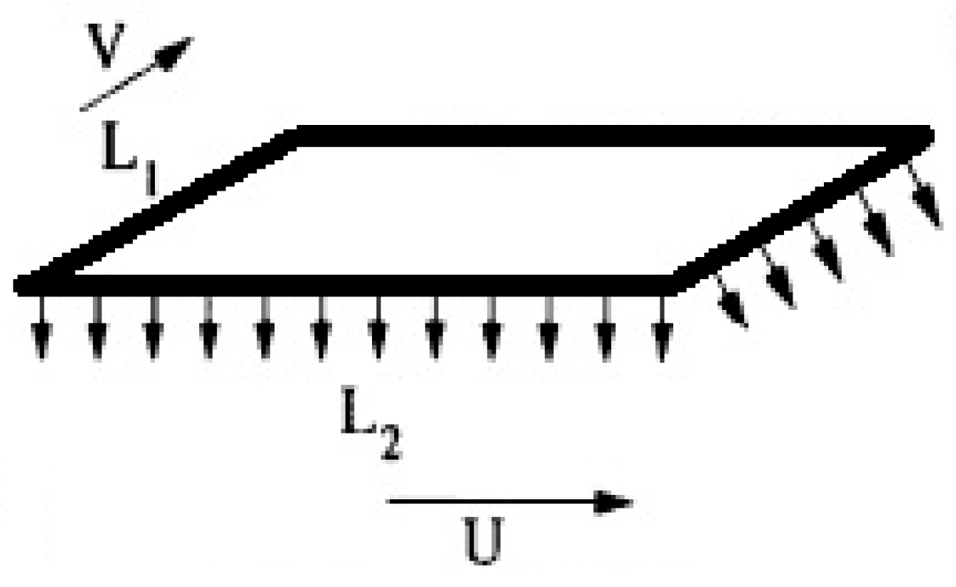
2. Problem Formulation

Consider a two dimensional LPS of dimensions L 1 and L 2 (Figure 1). The fluid is injected through the porous bottom to create a width φ with velocity b and slider velocities U (lateral) and V (longitudinal). The Navier-Stokes equations are:
· V = 0 ,
ρ ( V · ) V = p + d i v V
where ρ denotes the density of the fluid and p is the unknown part of the pressure, V = ( u , v , w ) , in which u , v and w are the velocity components of the fluid along x , y and z directions, respectively, and the del operator is defined as = ( x , y , z ) .
The boundary conditions are:
u = U , v = V , w = 0     at     η = 0
w = b , u = v = 0         at       η = φ .
We introduce the similarity transforms:
u = U f ( η ) + b h / ( η ) , v = V g ( η ) , w = b h ( η ) .
Assuming that L 2 L 1 φ , the end effects can be neglected. After substituting (5) in (4), (3), and (2), we obtain
h i v = R ( h / h / / h h / / / )
f / / = R ( f h / h f / )
g / / = R ( h g / )
R = b ξ / φ is the Reynolds number (R); η = ξ / φ is for transformation of the above equations into ordinary differential equations with the following boundary conditions:
h ( 0 ) = h / ( 0 ) = 0 , g ( 0 ) = f ( 0 ) = 1 , h ( 1 ) = 1 , h / ( 1 ) = g ( 1 ) = f ( 1 ) = 0

3. Integral Transform Method

To describe the formulation of Integral Transform Method (ITM), we consider the general nonlinear second order differential equation:
ψ / / ( η ) = f ( η , ψ ( η ) , ψ / ( η ) )
Along with the following boundary conditions:
η = α 0 :    ψ ( α 0 ) = α η = β 0    :    ψ ( β 0 ) = β
Integrating Equation (10) with respect to η from α 0 to η twice yields
ψ ( η ) = ψ ( α 0 ) + ( η α 0 ) ψ / ( α 0 ) + α 0 η ( η ζ ) f ( t , ψ ( ζ ) , ψ / ( η ) ) d ζ
ψ ( η ) = α + ( η α 0 ) ψ / ( α 0 ) + α 0 η ( η ζ ) f ( ζ , ψ ( ζ ) , ψ / ( ζ ) ) d ζ
By using second boundary condition we can evaluate ψ / ( α 0 ) , which is
ψ ( β 0 ) = β = α + ( β 0 α 0 ) ψ / ( α 0 ) + α 0 β 0 ( β 0 ζ ) f ( ζ , ψ ( ζ ) , ψ / ( ζ ) ) d ζ
( β α ) ( β 0 α 0 ) 1 ( β 0 α 0 ) α 0 β 0 ( β 0 ζ ) f ( ζ , ψ ( ζ ) , ψ / ( ζ ) ) d ζ = ψ / ( α 0 )
Substituting Equation (15) into (14) results in
ψ ( η ) = α + ( η α 0 ) [ ( β α ) ( β 0 α 0 ) 1 ( β 0 α 0 ) α 0 β 0 ( β 0 ζ ) f ( t , ψ ( ζ ) ) d t ] + α 0 η ( η ζ ) f ( ζ , ψ ( ζ ) , ψ / ( ζ ) ) d ζ
ψ ( η ) = ψ 0 ( η ) α 0 β 0 K ( η , ζ ) f ( ζ , ψ ( ζ ) , ψ / ( ζ ) ) d ζ ψ 0 ( η ) = α + ( η α 0 ) ( β α ) ( β 0 α 0 ) K ( η , ζ ) = ( η ζ ) ( β 0 α 0 ) ( η α 0 ) ( β 0 ζ ) ( β 0 α 0 ) ,   α 0 < ζ < η = ( η α 0 ) ( β 0 ζ ) ( β 0 α 0 ) , η < ζ < β 0   
Equation (17) is the standard form of variational iteration method-II. After applying this method, Equations (6) to (9) are expressed as follows
h ( η ) = 3 η 2 2 η 3 + 0 1 K ( η , ζ ) [ R ( h / h / / h h / / / ) ] d ζ K ( η , ζ ) = η 2 2 [ ( 1 ζ ) 3 ( 1 ζ ) 2 ] η 3 2 [ ( 1 ζ ) 2 2 3 ( 1 ζ ) 3 ] ( η ζ ) 3 3 ! , 0 < ζ < η = η 2 2 [ ( 1 ζ ) 3 ( 1 ζ ) 2 ] + η 3 2 [ ( 1 ζ ) 2 2 3 ( 1 ζ ) 3 ] , η < ζ < 1   
f ( η ) = 1 η + 0 1 K ( η , ζ ) R [ f h / h f / ] d ζ K ( η , ζ ) = ζ ( η 1 ) ,        0 < ζ < η = η ( 1 ζ )    ,      η < ζ < 1   
g ( η ) = 1 η 0 1 K ( η , ζ ) R [ h g / ] d ζ K ( η , ζ ) = ζ ( η 1 ) ,        0 < ζ < η = η ( 1 ζ )    ,      η < ζ < 1   
Furthermore, we can write Equations (18) to (20) in an iteration form as follows
h n + 1 = h 0 + 0 1 K ( η , ζ ) [ R ( h n / h n / / h n h n / / / ) ] d ζ w h e r e h 0 = 3 η 2 2 η 3 K ( η , ζ ) = η 2 2 [ ( 1 ζ ) 3 ( 1 ζ ) 2 ] η 3 2 [ ( 1 ζ ) 2 2 3 ( 1 ζ ) 3 ] ( η ζ ) 3 3 ! ,        0 < ζ < η                  = η 2 2 [ ( 1 ζ ) 3 ( 1 ζ ) 2 ] + η 3 2 [ ( 1 ζ ) 2 2 3 ( 1 ζ ) 3 ]                          ,      η < ζ < 1   
f n + 1 = f 0 + 0 1 K ( η , ζ ) [ f n h n / h n f n / ] d ζ w h e r e f 0 = 1 η K ( η , ζ ) = ζ ( η 1 ) ,    0 < ζ < η = η ( 1 ζ ) ,   η < ζ < 1
g n + 1 = g 0 0 1 K ( η , ζ ) [ h n g n / ] d ζ w h e r e g 0 = 1 η K ( η , ζ ) = ζ ( η 1 ) ,     0 < ζ < η = η ( 1 ζ ) ,    η < ζ < 1
By using the software MATHEMATICA, we calculated the series solution of the above mentioned problem. For reference, first few iterations of the problem are given in Appendix A.

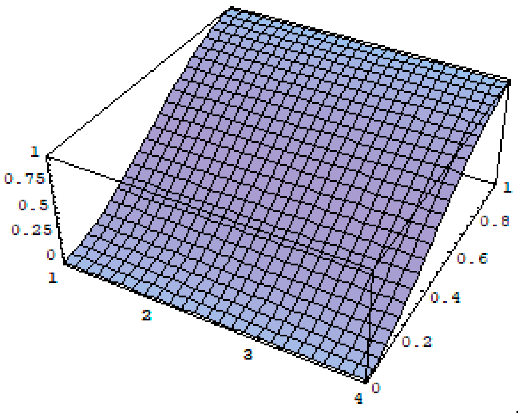
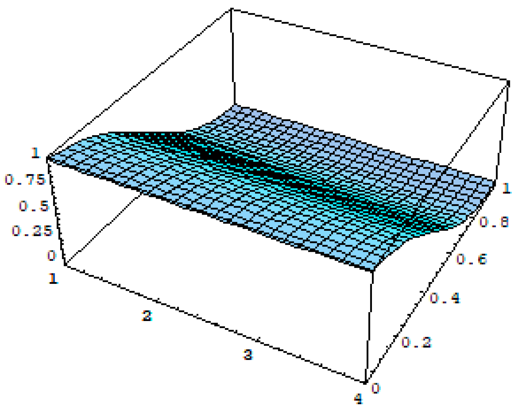
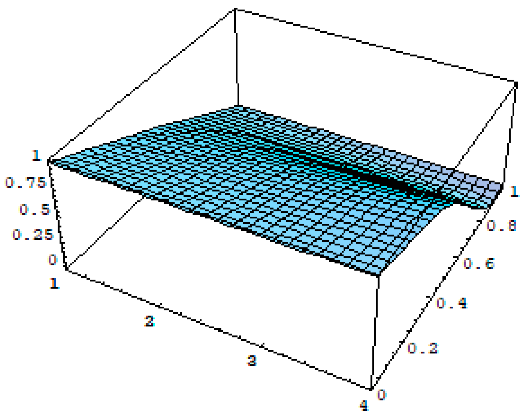
4. Graphs and Discussion

The graphical and numerical trend of h , f , and g are portrayed for 10th order approximation, which are calculated with Mathematica. Table 1, Table 2 and Table 3 present the direct comparison of the suggested method with existing methods. Through error analysis, we can see that ITM is showing close agreement with HAM (see Table 1, Table 2 and Table 3). Figure 2, Figure 3 and Figure 4 are plotted for different values of Reynolds Number, ranging from 1 to 4. Increasing Reynolds numbers result in increasing h and decreasing f (Figure 2 and Figure 3). According to Figure 3, g first increases and then decreases for increasing values of Reynolds numbers. Table 4 is consistent with the results obtained in the graphical description.

5. Conclusions

This paper presented a method for solving two-point nonlinear BVPs utilizing a recursive algorithm. This algorithm has the advantage of fewer calculations for obtaining the model parameters compared with VIM, HPM, ADM, and HAM. With this algorithm, a direct recursion scheme is obtained to solve the problem. This method is simple and does not have the difficulties that occur in numerical techniques, including perturbation, linearization, and discretizing the differential equations. The superiority of the presented method is demonstrated via comparison of error estimates with existing methods.

Author Contributions

First author (N.F.) conducted the whole research over all. It includes, mathematical work, writing the main manuscript. Second (Y.K.) and third authors (D.C.L.) helped to revise the reviewer comments, fourth author (M.G.) helped to improve the language of the paper.

Funding

This work was supported by International Cultural Exchange School (ICES) of Donghua University, West Yan’an Road 1882, Shanghai 200051, China.

Conflicts of Interest

The authors declare no conflict of interest.

Appendix A

By using software MATHEMATICS, we calculated first two terms for readers’ reference, which are as follows
h 1 = 3 η 2 2 η 3 93 η 5 10 33 η 6 5 + 144 R η 5 5 + 372 η 7 35 + 2169 R η 7 70 17 η 8 5 + 39 R η 8 5 16 η 9 7 + 48 R η 9 7 + 8 η 10 7 24 R η 10 7 1 70 η 2 ( η 1 ) 4 [ 13 + 3 R ( η 1 ) ( 1 2 η + 80 η 3 ) + 2 η ( 17 + η ( 29 40 ( 1 + η ) η ) ]
h 2 = 3 η 2 2 η 3 + 1 8408400 [ η 5 ( 372372 ( 1 + R ) ( 197 + 3 R ) 24024 ( 9456 + R ( 9004 + 375 R ) ) η + 5148 ( 46357 + R ( 43226 + 2739 R ) ) η 2 + 3003 ( 18248 + R ( 293795 + 246396 R ) ) η 3 1430 ( 739995 + R ( 3770264 + 2375319 R ) ) η 4 + 429 ( 6302956 + R ( 14667601 + 9657264 R ) ) η 5 + 546 ( 4376797 + R ( 31879751 + 9588621 R ) ) η 6 728 ( 20369787 + R ( 78989328 + 27702745 R ) ) η 7 + 336 ( 55114090 + 3 R ( 62573417 + 21934629 R ) ) η 8 2880 ( 2665268 + R ( 8412461 + 2975604 R ) ) η 9 147840 ( 13933 + R ( 50813 + 16759 R ) ) η 10 + 211200 ( 1 + 3 R ) ( 12479 + 4923 R ) η 11 5491200 ( 1 + 3 R ) ( 109 + 45 R ) η 12 ) ) ] + 1 8408400 [ ( ( 1 + η ) 4 η 2 ( 2 R 2 ( 1 + η ) ( 132531 + η ( 986440 + η ( 1453830 + η ( 3407635 + 4 η ( 1059779 + 6 η ( 6432489 + 40 η ( 217072 + 11 η ( 36583 + 270 η ( 287 + 130 η ) ) ) ) ) ) ) ) ) ) + R ( 119889 + η ( 213850 + η ( 1574734 + η ( 27839560 + η ( 22480115 + 2 η ( 131075 + 8 η ( 24782716 + 3 η ( 29019737 + 20 η ( 1178305 + 22 η ( 330131 + 240 η ( 1362 + 403 η ) ) ) ) ) ) ) ) ) ) ) 6 ( 188797 + η ( 405167 + η ( 487886 + η ( 3668210 + η ( 5523385 + η ( 1475047 + 4 η ( 359737 + 20 η ( 1001121 + 4 η ( 23838 + 11 η ( 89371 + 10 η ( 9645 + 2834 η ) ) ) ) ) ) ) ) ) ) ) ) ) ]
f 1 ( η ) = 1 η 2 R η 3 + 17 R η 4 4 61 R η 5 20 + 4 R η 6 5 + 1 20 ( 1 + η ) 2 η ( 3 + 6 η + 9 η 2 8 η 3 + 6 R ( 1 + η ) 2 ( 1 + 4 η ) )
f 2 ( η ) = 1 η 407 η 3 105 + R η 3 35 + 1241 η 4 168 19 R η 4 140 6129 η 5 1400 + 153 R η 5 700 + 607 η 6 700 389 R η 6 350 + 69 η 7 35 + 206 R η 7 35 229 η 8 70 12137 R η 8 560 2419 η 9 420 + 17995 R η 9 336 + 8293 η 10 420 166063 R η 10 2100 1132 η 11 55 + 127044 R η 11 1925 + 740 η 12 77 2220 R η 12 77 12 η 13 7 + 36 R η 13 7 + 1 92400 ( ( 1 + η ) 2 η ( 64511 ( 1 + 2 η ) 3 η 2 ( 70789 + η ( 23608 + 5 η ( 775 + η ( 930 + η ( 11851 + 4 η ( 1373 + 16 η ( 672 + 5 η ( 122 + 33 η ) ) ) ) ) ) ) ) + 2 R ( 2238 + η ( 4476 + η ( 1599 + η ( 5128 + η ( 12845 + η ( 109326 + η ( 230503 + 2 η ( 336389 + 144 η ( 4042 + 25 η ( 122 + 33 η ) ) ) ) ) ) ) ) ) ) ) )
g 1 ( η ) = 1 η 1 ( 3 R η 20 + 7 R η 4 4 12 R η 5 5 + 4 R η 6 5 )
g 2 ( η ) = 1 η ( 4769 R η 277200 1207 R 2 η 46200 13 R η 4 210 23 R 2 η 4 140 + 31 R η 5 280 + 129 R 2 η 5 560 9 R η 6 175 3 R 2 η 6 175 + 111 R 2 η 7 20 + 13 R η 8 10 643 R 2 η 8 35 1983 R η 9 560 + 13901 R 2 η 9 560 + 1163 R η 10 315 1807 R 2 η 10 105 61 R η 11 35 + 1083 R 2 η 11 175 + 24 R η 12 77 72 R 2 η 12 77 1 140 R ( 1 + η ) ( 1 4 ( 26 + 69 R ) η 4 + 12 5 ( 3 + 5 R ) η 5 + 666 R η 7 7 4 ( 91 + 953 R ) η 8 + 4 9 ( 673 + 3615 R ) η 9 + ( 196 3612 R 5 ) η 10 + 480 11 ( 1 + 3 R ) η 11 )

References

  1. Nadeem, S.; Haq, R.U.; Akbar, N.S.; Khan, Z.H. MHD three-dimensional Casson fluid flow past a porous linearly stretching sheet. Alex. Eng. J. 2013, 52, 577–582. [Google Scholar] [CrossRef]
  2. Khan, Y.; Faraz, N.; Yildirim, A.; Wu, Q. A series solution of the long porous slider. Tribol. Trans. 2011, 54, 187–191. [Google Scholar] [CrossRef]
  3. Faraz, N. Study of the effects of the Reynolds number on circular porous slider via variational iteration algorithm-II. Comput. Math. Appl. 2011, 61, 1991–1994. [Google Scholar] [CrossRef] [Green Version]
  4. Rao, P.S.; Agarwal, S. Effect of permeability and different slip velocities at both the porous interface using couple stress fluids on the slider bearing load carrying mechanism. Proc. Inst. Mech. Eng. Part J J. Eng. Tribol. 2016, 230, 196–201. [Google Scholar] [CrossRef]
  5. Kumar, S.; Pai, N. Analysis of Porous Eliptical Slider through Semi-Analytical Technique. J. Adv. Res. Fluid Mech. Therm. Sci. 2018, 48, 80–90. [Google Scholar]
  6. Zhu, Z.; Nathan, R.; Wu, Q. Multi-scale soft porous lubrication. Tribol. Int. 2019, 137, 246–253. [Google Scholar] [CrossRef]
  7. Lang, J.; Nathan, R.; Wu, Q. Theoretical and experimental study of transient squeezing flow in a highly porous film. Tribol. Int. 2019, 135, 259–268. [Google Scholar] [CrossRef]
  8. Bujurke, N.M.; Patil, H.P.; Bhavi, S.G. Porous slider bearing with couple stress fluid. Acta Mech. 1990, 85, 99–113. [Google Scholar] [CrossRef]
  9. Wang, C.Y. A porous slider with velocity slip. Fluid Dyn. Res. 2012, 44, 065505. [Google Scholar] [CrossRef]
  10. Honchi, M.; Kohira, H.; Matsumoto, M. Numerical simulation of slider dynamics during slider-disk contact. Tribol. Int. 2003, 36, 235–240. [Google Scholar] [CrossRef]
  11. Shah, R.C.; Bhat, M.V. Ferrofluid lubrication in porous inclined slider bearing with velocity slip. Int. J. Mech. Sci. 2002, 44, 2495–2502. [Google Scholar] [CrossRef]
  12. Awati, V.B.; Jyoti, M. Homotopy analysis method for the solution of lubrication of a long porous slider. Appl. Math. Nonlinear Sci. 2016, 1, 507–516. [Google Scholar] [CrossRef] [Green Version]
  13. Khan, Y.; Wu, Q.; Faraz, N.; Yildirim, A.; Mohyud-Din, S.T. Three-dimensional flow arising in the long porous slider: An analytic solution. Z. Naturforsch. 2011, 66, 507–511. [Google Scholar] [CrossRef]
  14. Turkyilmazoglu, M. Some issues on HPM and HAM methods: A convergence scheme. Math. Comput. Model. 2011, 53, 1929–1936. [Google Scholar] [CrossRef]
  15. Safari, M.; Ganji, D.D.; Moslemi, M. Application of He’s variational iteration method and Adomian’s decomposition method to the fractional KdV-Burgers-Kuramoto equation. Comput. Math. Appl. 2009, 58, 2091–2097. [Google Scholar] [CrossRef]
  16. Faraz, N.; Khan, Y. Study of the dynamics of rotor-spun composite yarn spinning process in forced vibration. Text. Res. J. 2012, 82, 255–258. [Google Scholar] [CrossRef]
Figure 1. Schematic diagram of moving long porous slider.
Symmetry 11 00791 g001
Figure 2. Effect of Reynolds number on velocity component h.
Symmetry 11 00791 g002
Figure 3. Effect of Reynolds number on velocity component f.
Symmetry 11 00791 g003
Figure 4. Effect of Reynolds number on velocity component g.
Symmetry 11 00791 g004
Table 1. Comparison with homotopy Padé approximation method [12] for larger Reynolds numbers.
HAM [12]PresentError
R h / / / ( 0 )
0.212.465334166512.465334166−5E-10
114.36534665414.365346654−0E+0
216.823567355516.8235673555−0E+0
319.356545855819.3565458558−0E+0
421.947351077221.9473510772−0E+0
524.583070789124.55234070789−5E-10
627.253310982527.2533109818−7E-10
729.947695116329.9476951136−2.7E-9
832.661163241632.6611632329−8.7E-9
935.392471009735.3924709848−2.49E-8
1038.144912550738.1449125256−2.51E-8
51.6149.6714726105149.6714725836−2.69E-8
70197.9636925814197.9636925523−2.91E-8
100275.9321654987275.9321651777−3.21E-7
300788.4398765432788.4398762142−3.29E-7
5001291.11592634871289.1236547891−1.99
10002526.42398.1243−128.27
Table 2. Comparison with homotopy Padé approximation method [12] for larger Reynolds numbers.
HAM [12]PresentError
R f / ( 0 )
0.21.08802583691.0880258369-0E-0
11.40536925811.4053692581-0E+0
21.74453216541.7445321654-0E+0
32.03611592632.0361159263-0E+0
42.28667534212.2866753421-0E+0
52.52874185292.5287418529-0E-0
62.91369852142.9136985214-0E-0
73.1728396543.172839654-0E-0
83.65432198713.6543219866-5E-10
93.82937112343.8293711226-8E-10
104.11258369174.1125836759-1.58E-8
51.67.55314725837.5531472314-2.69E-8
708.75735724198.7573572108-3.11E-8
10010.4014731110.401472583-5.27E-7
30017.8153700717.815369258-8.12E-7
50022.67022.661-0.009
100030.43230.429-3.00
Table 3. Comparison with homotopy Padé approximation method [12] for larger Reynolds numbers.
HAM [12]PresentError
R g / ( 0 )
0.21.03012583691.0301258369-0E-0
11.15319516231.1531951623-0E+0
21.30963147851.3096314785-0E+0
31.46589516231.4658951623-0E+0
41.61872583691.6187258369-0E+0
51.7661597411.766159741-0E-0
61.90864563211.9086456321-0E-0
72.04641582312.0464158231-0E-0
82.18504741252.1850474125-0E-0
92.33681159872.3368115987-0E-0
102.52643147552.5264314755-0E-0
51.65.30114632955.30114632825-1.25E-9
706.14492366816.144923667892.1E-8
1007.28815835417.2881580341-3.27E-7
30012.516125812.5160446-8.12E-5
50015.36812415.258154-010997
100020.06219.1583-0.9037
Table 4. Comparison between HPM, Numerical (Num.), and the presented technique for different Reynolds numbers.
HAM [12]Num. [9]PresentHPM [12]Num. [9]PresentHPM [12]Num. [9]Present
R h / / / ( 0 ) f / ( 0 ) g / ( 0 )
0.212.46512.46512.4651.08801.0881.0881.03011.03011.030
114.36514.36514.3651.4051.4051.4051.15311.1531.153
2--16.8235--1.7445--1.30963
3--19.356--2.0361--1.4658
4--21.9473--2.2866--1.6187
524.58624.58424.5842.44172.5282.528--1.766
6--27.253-----1.9086
7--29.9476-----2.04641
8--32.6611-----2.18504
9--35.3924-----2.33681
10--38.1449-----2.52643
11--40.9267-----2.79796
12--43.7471-----3.2218
13.848.904348.48448.4844.02294.0224.022--4.70844
15--52.2461-----6.53822
16--54.6612-----8.72019
51.6149.67149.67149.677.5537.5537.5535.3015.3015.301

