Abstract
In the work, a nonlinear reaction-diffusion model in a class of delayed differential equations on the hexagonal lattice is considered. The system includes a spatial operator of diffusion between hexagonal pixels. The main results deal with the qualitative investigation of the model. The conditions of global asymptotic stability, which are based on the Lyapunov function construction, are obtained. An estimate of the upper bound of time delay, which enables stability, is presented. The numerical study is executed with the help of the bifurcation diagram, phase trajectories, and hexagonal tile portraits. It shows the changes in qualitative behavior with respect to the growth of time delay; namely, starting from the stable focus at small delay values, then through Hopf bifurcation to limit cycles, and finally, through period doublings to deterministic chaos.
1. Introduction
Currently, reaction-diffusion models are used in the design and study of many detecting, measuring, and sensing devices. Immunosensors, which are studied here as an example, represent a kind of them. Such spatial-temporal models are described by the systems of partial or lattice differential equations.
The reaction-diffusion models are traditionally studied from the viewpoint of their qualitative analysis. Even in the case of a small number of spatial elements, they show complex behavior. In [1], it was shown that the model describing the chemical reaction of two morphogens (reactants), one of them diffusing within two compartments, resulted in “bi-chaotic” behavior. The origin of such chaotic phenomena (They called it “spiral turbulence” in [2]) were also explained with the help of the statistics of topological defects [2].
When considering continuously-distributed reaction-diffusion models described by nonlinear partial differential equations, the Feigenbaum–Sharkovskii–Magnitskii bifurcation theory can be applied, which results in a subharmonic cascade of bifurcations of stable limit cycles [3].
The lattice differential equations describe systems with a discrete spatial structure, which is more consistent with pixel devices. These equations were also called earlier by a series of authors spatially-discrete differential equations [4].
Due to [5], a typical lattice differential equation takes the form:
where we consider a lattice , which can be presented as a discrete subset of , consisting of either a finite or infinite number of points, which are located in accordance with some regular spatial structure. The vectors , are the values of the state , calculated at the the points of the lattice, and are the right sides of the equations with the properties enabling us to find the existence of the solution.
As a rule, without loss of generality, these consider , which is the integer lattice in . The methods developed can be easily applied to a different type of lattice, namely the planar rectangular and hexagonal lattice, the crystallographic lattices in .
These pay attention to the notion of delay in lattice differential equations, the so-called delayed lattice differential equations. One of the applications dealing with them is the investigation of traveling wave fronts and their stability [5]. The main results are applied to the delayed and discretely diffusive models for the population (see, e.g., [6,7]).
Lattice differential equations are used as models in many applications, for example cellular neural networks, image processing, chemical kinetics, materials science, in particular metallurgy, and biology [5,8]. Lattice models are extremely attractive from the viewpoint of population dynamics, especially in the case of spatially-separated populations [5,6,8,9,10,11].
There are a few reasons for requiring the consideration of the hexagonal grid instead of rectangular one (primarily in image and vision computing); namely, the equal distances between neighboring pixels for hexagonal coordinate systems [12]; hexagonal points are packed more densely [13]; since “hexagons are ‘rounder’ than squares”, the presentation of curves is more consistent with the help of hexagonal systems [13]; hence, mathematical operations of edge detection and shape extraction are more successful when applying hexagonal lattices [14].
With the purpose of indexing hexagonal pixels, as a rule, two-(This is the so-called “skewed-axis” coordinate system) or three-element (It is also known as the “cube hex coordinate system”) coordinate systems have been used [15]. Our reasoning will be based on the last one. Contrary to the skewed axes, using the cubic coordinates enables us to obtain symmetries with respect to all three axes.
Note that one-element coordinate systems for hexagonal grids are also possible. With this purpose, in [16], the spiral architecture based on a single dimensional addressing system was offered.
The aim of this work is to construct one hexagonal model of the reaction-diffusion type, which describes the hexagonal lattice of immunopixels and to study its qualitative behavior when changing parameters.
2. Lattice Reaction-Diffusion Model on a Hexagonal Biopixel Array
The model, which is further presented, describes the antigen-antibody interaction, which is the base of the immune reaction used for the construction of immunopixels. Such a model can be applied to general predator-prey models of population dynamics. The model was studied in the case of the rectangular lattice in [17]. Therefore, here, we will compare numerically the influence of the hexagonal lattice on the stability properties of the immunosensor.
Therefore, we consider hexagonal lattice of immunopixels, which are indexed by the three-element coordinates , where , , . Let be the antigen concentration, be the antibody concentration within biopixel , and , . Given biopixel , we make the following assumptions with respect to the immune reaction.
- Antigens are born with the constant birthrate .
- We have some probability rate for the binding of antigens with antibodies.
- The antigen population tends to some carrying capacity with the rate .
- Antibodies die with the constant birthrate .
- As a result of immune response, we have the increase of the density of antibodies with probability rate .
- The antibody population tends to some carrying capacity with rate .
- The immune response appears with some constant time delay .
Antigens are assumed to diffuse from six neighboring pixels, , , , , , (see Figure 1), with diffusion rate , where , and is the distance between pixels.
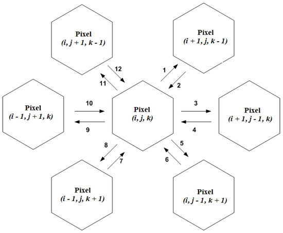
Figure 1.
Diffusion of antigens for the hexagonal lattice model. Antigens from six neighboring pixels interact. is the constant of disbalance. Here, ‘1’, ‘3’, ‘5’, ‘8’, ‘9’, ‘11’ have to be replaced with , ‘2’ with , ‘4’ with , ‘6’ with , ‘7’ with , ‘10’ with , and ‘12’ with .
Taking into account the prerequisites mentioned above, we obtain a simplified antibody-antigen competition model with delay for a hexagonal array of biopixels, which uses the Marchuk model of the immune response [18,19,20,21] and the spatial operator , which is constructed similarly to [22] (Supplementary Information, p. 10).
with given initial functions:
We use the following spatial operator of discrete diffusion for a hexagonal array of pixels:
Each pixel is affected by the antigens flowing out of six neighboring pixels, two in each of three directions of the hexagonal array. The adjoint pixels are separated by the distance .
Boundary conditions for the edges of the hexagonal array, i.e., if , are used.
Section 3 and Section 4 present analytical results with respect to the model (2) in the form of restrictions for the parameters, enabling us persistence and global asymptotic stability. Moreover, Section 5 offers numerical research of the system’s qualitative behavior with dependence on the changes of the time of immune response (time delay), diffusion rate , and factor n.
3. Persistence of the Solutions
We use the following definition, which generalizes [23] for lattice differential equations.
Definition 1.
System (2) is said to be uniformly persistent if for all , , there exist compact regions such that every solution , , of (2) with the initial conditions (3) eventually enters and remains in the region .
Lemma 1.
Let , be the solutions of (2) with initial conditions (3). If:
then:
for some large values of t. Here:
Proof.
Firstly, we can prove that there exists some large instant of time such that , , , .
Let us assume the contrary, i.e., there is , such that at , which is a contradiction with the balance principle.
Since the solutions of the system (2) and (3) are positive, then:
Further, we can apply the basic steps of the proof of Lemma 3.1 [24], which is proven in the non-lattice case (i.e., without the spatial operator). □
Remark 1.
The conditions of the uniform persistence of System (2) in the non-lattice case were obtained in [25]. They resulted in Inequality (5) provided that:
holds.
4. Stability Problem in Immunosensors
Stability from a biosensor point of view is very important. With respect to biosensors, two notions of stability are introduced. Namely, these are self-stability and operational stability.
Self-stability characterizes the sustainability of the biosensor for a long period of time. To check the self-stability of the biorecognition element, measurements of the response of the biosensor to the same amount of measurands are fulfilled.
Operational stability shows the identity of the sensor response to the same substrate concentration when conducting a large number of consecutive measurements [26] and is closely related to the metrological characteristic of convergence (repeatability). The operational stability of the sensors is characterized by a relative standard deviation with repeated measurements of the standard sample and the residual activity of the biosensor after several consecutive measurements over a certain period of time.
The results, which are presented in the work, could be applied to study both types of biosensor stabilities. Namely, with help of the changing initial conditions, we can simulate different circumstances to investigate its qualitative behavior.
4.1. Steady States
The steady states can be calculated as a result of solving , , , with respect to the model (2).
Prey-free steady state: In case of the absence of antigens (preys), , we have two possible opportunities, namely, either , or , , . The last one is of biological meaning and is not reachable for positive initial values (3).
In order to get an endemic state , , of (2), the following system of algebraic equations has to be solved:
The solving of (10) with respect to results in the system of algebraic lattice equations for and taking into account the dependence .
Analyzing the solutions, two types of endemic steady states are differed.
Pixel-independent endemic state: In the case of the existence of solutions of (10), which are identical for all pixels, i.e., , , , , the endemic steady states , are presented as:
provided that .
Pixel-dependent endemic state: Because of the diffusion between pixels , the endemic steady states are not equal to (11), and in Section 5, it is evidenced numerically.
For the diffusion-free system, i.e., , pixel-independent endemic states are observed for pixels on the hexagonal boundary.
If , we get pixel-dependent endemic steady states for the internal pixels, which converge to the pixel-independent ones (11). Numerical study shows that the bigger the number N, the clearer is the appearance of pixel-dependent endemic states.
4.2. Global Asymptotic Stability
Here, the global asymptotic stability of the positive endemic steady state , , is investigated.
Theorem 1.
Assume that:
and:
Then, the positive endemic steady state , of system (2) is globally asymptotically stable.
Proof.
We use the change of the variables:
This implies:
Substituting (13) into (2), we get:
This yields:
Since:
then:
Let .
Rewrite the first equation as:
For arbitrary pixel , , consider the Lyapunov functionals:
Then, we have for the right-upper derivative along (18):
By Lemma 1, we know that there exists a such that for , and hence, for ,
Next, let:
Then, we have at :
Rewrite the second equation (17) as:
For arbitrary pixel , , , consider the Lyapunov functionals:
Then, we have for right-upper derivative along (20):
Considering for arbitrary pixel , , the Lyapunov functional , we have for the right-upper derivative along (20):
Let us consider:
Since is the steady state, we see that for any arbitrary small , there is some instant of time such that:
Further, we consider and omit in (23) without lost of generality.
We have:
Let . Then, calculating the derivative of along the solutions of (20), we have:
□
Corollary 1.
Assume that the conditions of Theorem 1 are true. Then, the positive equilibrium state , , of System (2) is globally asymptotically stable at , where:
Remark 2.
The conditions of the global asymptotic stability of the endemic steady state , , of system (2) are dependent on the diffusion rate D, the distance between pixels Δ, and the disbalance constant n.
5. Numerical Study
For the numerical simulation, we consider Model (2) of the hexagonal pixel array at , = 2 min−1, = 2 , = 1 min−1, , = 0.5 , = 0.5 , D = 0.2 , nm. Numerical modeling was implemented at different values of . For this purpose, we used the RStudio environment.
Using the local bifurcation plot, the dynamics of the system (2) was analyzed for different values of (see Figure 2). We concluded that oscillatory and then chaotic behavior starts for smaller values of at smaller values of n. Further, increasing the values of n, we can observe asymptotically stable steady solutions for a wider range of .
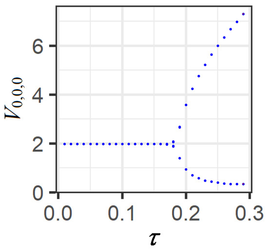
Figure 2.
Bifurcation plot for at .
Numerical integration of the system have shown the influence of time delay . Namely, as it agrees with our analytical results of Section 4, we observe the stable focuses at pixel-dependent endemic states for small delays (see Figure 3).
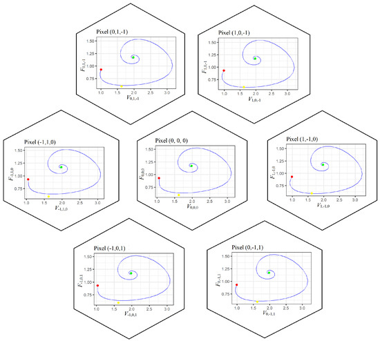
Figure 3.
Phase plots of the system (2) at , which correspond to stable focus. Here, ● indicates the initial state, ● the pixel-independent endemic state, and ● the pixel-dependent endemic state.
At min, the stable focus is transformed into a stable limit cycle of tiny radius, which corresponds to Hopf bifurcation. A deeper study of this phenomenon requires obtaining the condition of the appearance of the pair of purely imaginary roots of the characteristic quasipolynomial of the linearized system. The limit cycles of the ellipsoidal form are observed till min (see Figure 4 for ). Notice that when increasing , near , we get period doubling (see Figure 5) (It can be approximately seen from local bifurcation plot also.).
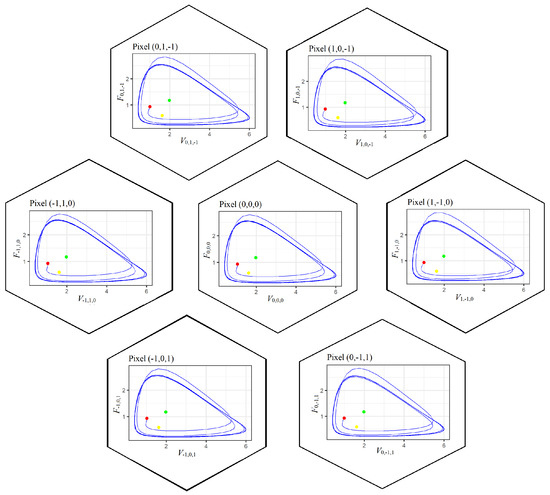
Figure 4.
Phase plots of the system (2) at . The solution tends to a stable limit cycle. Here, ● indicates the initial state, ● the pixel-independent endemic state, and ● the pixel-dependent endemic state.
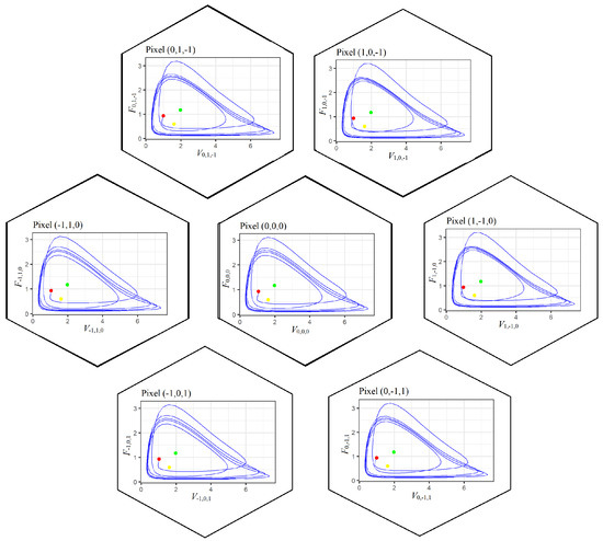
Figure 5.
Phase plots of the system (2) at . Here, ● indicates the initial state, ● the pixel-independent endemic state, and ● the pixel-dependent endemic state. The solution tends to a stable limit cycle with six local extrema per cycle.
The qualitative behavior of the immunosensor model can be analyzed with the help of hexagonal tiling plots as well. For this purpose, we can use both plots for antigens (Figure 6), antibodies (Figure 7), and the probabilities of binding antigens by antibodies (Figure 8).
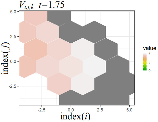
Figure 6.
Example of the hexagonal tiling plot for V.
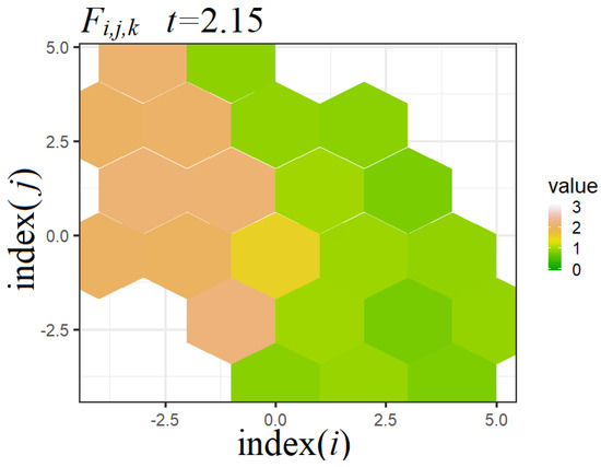
Figure 7.
Example of the hexagonal tiling plot for F.
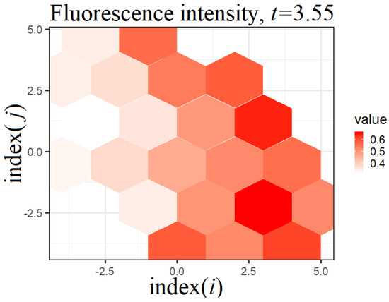
Figure 8.
Example of the hexagonal tiling plot for the probabilities of binding antigens by antibodies, i.e., . In the case of the optical immunosensor, it is fluorescence intensity.
6. Conclusions
In this work, a reaction-diffusion model of a hexagonal immunosensor was considered. Mathematically, it was described by the system of lattice delayed differential equations on the hexagonal grid. The system included the spatial operator describing the diffusion of antigens between pixels.
The main results dealt with the qualitative investigation of the model. The conditions of the global asymptotic stability were obtained. These used the construction of the Lyapunov functional. These resulted in an inequality, including the system parameters and delay. Therefore, the estimation of the delay enabling the global asymptotic stability can be obtained.
Numerical analysis of the model was performed with the help of the bifurcation diagram, phase trajectories, and hexagonal tile portraits. The changes in the qualitative behavior with respect to the growth of the time delay were shown; namely, starting from the stable focus at small delay values, then through Hopf the bifurcation to limit cycles, and finally, through period doublings to deterministic chaos. This agreed with the results on space-time chaos for reaction-diffusion systems, which were previously obtained in [1,2,3].
As compared with the rectangular lattice model studied in [17], for the hexagonal model, we observed Hopf bifurcation at smaller values of . That is, the hexagonal lattice accelerated changes in qualitative behavior.
Note that the model can be applied for an arbitrary amount of pixels determined by natural . However, it can be numerically seen that the qualitative behavior of the entire immunosensor was determined by a seven-pixel array.
Author Contributions
Conceptualization, V.M. and O.V.; methodology, V.M. and O.V.; software, V.M. and O.V.; validation, V.M. and O.V.; formal analysis, V.M. and O.V.; investigation, V.M. and O.V.; resources, V.M. and O.V.; data curation, V.M. and O.V.; writing, original draft preparation, V.M. and O.V.; writing, review and editing, V.M. and O.V.; visualization, V.M. and O.V.; supervision, V.M.; project administration, V.M.; funding acquisition, V.M. and O.V.
Funding
The work is supported by the University of Bielsko-Biala, Program Number 511/100/4/10/00.
Acknowledgments
The authors are thankful to the reviewers for significant comments and remarks.
Conflicts of Interest
The authors declare no conflict of interest.
References
- Rössler, O.E. Chemical Turbulence: Chaos in a Simple Reaction-Diffusion System. Z. Naturforsch. A 1976, 31. [Google Scholar] [CrossRef]
- Hildebrand, M.; Bär, M.; Eiswirth, M. Statistics of Topological Defects and Spatiotemporal Chaos in a Reaction-Diffusion System. Phys. Rev. Lett. 1995, 75, 1503–1506. [Google Scholar] [CrossRef] [PubMed]
- Zaitseva, M.F.; Magnitskii, N.A. Space–time chaos in a system of reaction–diffusion equations. Differ. Equ. 2017, 53, 1519–1523. [Google Scholar] [CrossRef]
- Cahn, J.W.; Chow, S.; Van Vleck, E.S. Spatially discrete nonlinear diffusion equations. Rocky Mount. J. Math. 1995, 25, 87–118. [Google Scholar] [CrossRef]
- Chow, S.N.; Mallet-Paret, J.; Van Vleck, E.S. Dynamics of lattice differential equations. Int. J. Bifurc. Chaos 1996, 6, 1605–1621. [Google Scholar] [CrossRef]
- Pan, S. Propagation of delayed lattice differential equations without local quasimonotonicity. Ann. Pol. Math. 2015, 114, 219–233. [Google Scholar] [CrossRef][Green Version]
- Huang, J.; Lu, G.; Zou, X. Existence of traveling wave fronts of delayed lattice differential equations. J. Math. Anal. Appl. 2004, 298, 538–558. [Google Scholar] [CrossRef]
- Niu, H. Spreading speeds in a lattice differential equation with distributed delay. Turk. J. Math. 2015, 39, 235–250. [Google Scholar] [CrossRef]
- Hoffman, A.; Hupkes, H.; Van Vleck, E. Entire Solutions for Bistable Lattice Differential Equations with Obstacles; American Mathematical Society: Providence, RI, USA, 2017. [Google Scholar]
- Wu, F. Asymptotic speed of spreading in a delay lattice differential equation without quasimonotonicity. Electron. J. Differ. Equ. 2014, 2014, 1–10. [Google Scholar]
- Zhang, G.B. Global stability of traveling wave fronts for non-local delayed lattice differential equations. Nonlinear Anal. Real World Appl. 2012, 13, 1790–1801. [Google Scholar] [CrossRef]
- Luczak, E.; Rosenfeld, A. Distance on a hexagonal grid. IEEE Trans. Comput. 1976, 25, 532–533. [Google Scholar] [CrossRef]
- Hexagonal Coordinate Systems. Available online: https://homepages.inf.ed.ac.uk/rbf/CVonline/LOCAL_COPIES/226AV0405/MARTIN/Hex.pdf (accessed on 12 May 2019).
- Middleton, L.; Sivaswamy, J. Edge detection in a hexagonal-image processing framework. Image Vis. Comput. 2001, 19, 1071–1081. [Google Scholar] [CrossRef]
- Fayas, A.; Nisar, H.; Sultan, A. Study on hexagonal grid in image processing. In Proceedings of the 4th International Conference on Digital Image Processing, Kuala Lumpur, Malaysia, 7–8 April 2012; pp. 7–8. [Google Scholar]
- Middleton, L.; Sivaswamy, J. Hexagonal Image Processing: A Practical Approach; Springer Science & Business Media: New York, NY, USA, 2006. [Google Scholar]
- Martsenyuk, V.; Kłos-Witkowska, A.; Sverstiuk, A. Stability, bifurcation and transition to chaos in a model of immunosensor based on lattice differential equations with delay. Electron. J. Qual. Theory Differ. Equ. 2018, 2018, 1–31. [Google Scholar] [CrossRef]
- Marchuk, G.; Petrov, R.; Romanyukha, A.; Bocharov, G. Mathematical model of antiviral immune response. I. Data analysis, generalized picture construction and parameters evaluation for hepatitis B. J. Theor. Biol. 1991, 151, 1–40. [Google Scholar] [CrossRef]
- Foryś, U. Marchuk’s Model of Immune System Dynamics with Application to Tumour Growth. J. Theor. Med. 2002, 4, 85–93. [Google Scholar] [CrossRef]
- Nakonechny, A.; Marzeniuk, V. Uncertainties in medical processes control. Lect. Notes Econ. Math. Syst. 2006, 581, 185–192. [Google Scholar] [CrossRef]
- Marzeniuk, V. Taking into account delay in the problem of immune protection of organism. Nonlinear Anal. Real World Appl. 2001, 2, 483–496. [Google Scholar] [CrossRef]
- Prindle, A.; Samayoa, P.; Razinkov, I.; Danino, T.; Tsimring, L.S.; Hasty, J. A sensing array of radically coupled genetic ‘biopixels’. Nature 2011, 481, 39–44. [Google Scholar] [CrossRef]
- Kuang, Y. Delay Differential Equations with Applications in Population Dynamics; Academic Press: New York, NY, USA, 1993. [Google Scholar]
- He, X.Z. Stability and Delays in a Predator-Prey System. J. Math. Anal. Appl. 1996, 198, 355–370. [Google Scholar] [CrossRef]
- Wendi, W.; Zhien, M. Harmless delays for uniform persistence. J. Math. Anal. Appl. 1991, 158, 256–268. [Google Scholar] [CrossRef]
- Gibson, T.D. Biosensors: The stabilité problem. Analusis 1999, 27, 630–638. [Google Scholar] [CrossRef]
© 2019 by the authors. Licensee MDPI, Basel, Switzerland. This article is an open access article distributed under the terms and conditions of the Creative Commons Attribution (CC BY) license (http://creativecommons.org/licenses/by/4.0/).