Abstract
A data-driven adaptive iterative learning (IL) method is proposed for the active control of structural vibration. Considering the repeatability of structural dynamic responses in the vibration process, the time-varying proportional-type iterative learning (P-type IL) method was applied for the design of feedback controllers. The model-free adaptive (MFA) control, a data-driven method, was used to self-tune the time-varying learning gains of the P-type IL method for improving the control precision of the system and the learning speed of the controllers. By using multi-source information, the state of the controlled system was detected and identified. The square root values of feedback gains can be considered as characteristic parameters and the theory of imprecise probability was investigated as a tool for designing the stopping criteria. The motion equation was driven from dynamic finite element (FE) formulation of piezoelectric material, and then was linearized and transformed properly to design the MFA controller. The proposed method was numerically and experimentally tested for a piezoelectric cantilever plate. The results demonstrate that the proposed method performs excellent in vibration suppression and the controllers had fast learning speeds.
1. Introduction
Many industrial systems accomplish tasks in a limited period of time and repeat control processes continuously. In these systems, it is attractive to improve the system performance by repeating the control process, which draws attention to intelligent control strategy, named the iterative learning (IL) method. The IL method is applicable to controlled systems with repetitive motion properties. The fundamental IL method is a learning process based on output errors and learning gains. To obtain better control performances, the upgraded system inputs will be generated at the next repetitive processes by the latest tracking errors [1]. In practical industrial processes, the IL method is an effective approach to produce the control inputs, so the system outputs are as close as possible to the desired system outputs, such as: control trajectory tracking for lower limb rehabilitation [2], design of a shaping method for the residual vibration control of industrial robots [3], compensation for aerodynamic disturbance of the aerial refueling system [4], design of the controller for homing guidance of missiles [5]. Considering the repeatability of structural dynamic responses in the vibration process, several research groups have applied the proportional-type iterative learning (P-type IL) method with fixed gain to suppress the vibrations of piezoelectric laminated composite structures. The P-type IL method was first applied to vibration active control of piezoelectric structures by Zhu et al. [6] and Tavakolpour et al. [7], and its control performance has also been studied. Zhang et al. [8] designed a controller to compensate the disturbance estimation and disturbance rejection, where the P-type IL method was used to estimate the system position.
In the P-type IL method, thousands of iterations are necessary to obtain the desired control precision, which may reduce the convergence speed [7,9]. It is worth pointing out that the systems will spillover or even become unstable in practice applications, as the fixed-learning gain are selected unreasonably [10]. For improving the convergence speed and the system stability, the adaptive control is necessary to design the optimal learning gain in each iteration. To design vibration active control systems, both control strategies and structure characteristics need to be seriously considered. Piezoelectric flexible structures, such as plates and shells, challenge researchers in vibration active control for their complexity in the vibration modes [11,12,13]. In addition, using one single actuator–sensor pair bonded on a plate is obviously unreasonable to suppress all vibration modes and to identify dynamic responses for all locations on the plate. A distributed method that piezoelectric actuator-sensor pairs at discrete locations were bonded on the plate was constructed [14]. Piezoelectric laminated composite structures have low weight and cannot achieve great changes in the dynamic characteristics of the plate. A flexible plate with several piezoelectric actuator–sensor pairs, thus, is a multi-input–multi-output (MIMO) system. If a piezoelectric actuator is not able to satisfactorily perform the given task, the actuators nearby will be influenced negatively. The interaction between actuators will exist in the entire operating process of the system, and the information of the interaction will be uncertain. The obstacle in dealing with the system uncertainty challenges the model-based methods.
A model-free adaptive (MFA) control, a data-driven adaptive control method, can be operated using only input and output (I/O) data from the system [15] and is suitable to deal with uncertainties [16].Such a method can realize the adaptive adjust in parametric as well as structural manners, and have been successfully incorporated into the IL method for different industrial applications, such as particle quality control for spray fluidized-bed granulation [17], formation control of multi-agent systems [18],freeway traffic iterative learning control [19], and vibration suppression [20]. In this paper, the MFA control was applied to tune the learning gains of the P-type IL method by the system’s dynamic behavior. The P-type IL method with time-varying learning gains was used to design the feedback gains, which can accelerate the convergence speed.
To avoid system spillover, the feedback gains must be converged to appropriate values after a period of time. The convergence properties of the controlled system should be seriously considered. The conventional P-type IL method has two domains, namely, time domain and iteration domain. The task of a conventional P-type IL method is implemented in a finite-time interval. Thus, the convergence of the control system in the time domain is not considered, while the convergence of the control system in the iteration domain is focused on. In this paper, the proposed method was different from the conventional P-type IL method, which has only a single domain. In other words, the time domain and iteration domain of the proposed method were overlapping. The convergence properties of the proposed method in overlapping domain need to be considered seriously; however, the convergence analysis in the overlapping domain is still an open problem. Bai et al. [20] designed stopping criteria to guarantee that feedback gains can converge to the appropriate values using the evidence theory. Based on the evidence theory, decision-makings on system states can be carried out by comparing threshold values. However, the results of decision-making are counterintuitive when the given evidence is conflicting [21,22]. In addition, dealing with conflict in evidence theory is still an open question. To make the learning process of feedback gains smoother and to reduce conflicting evidence caused by external noise, sliding mode control (SMC) is used to compensate learning gain in real time [20]. However, the introduction of SMC brings a great computational burden, which results in a great time delay. Generally speaking, the more actuator–sensor pairs that are bonded on the plate, the more the vibration modes of the plate which can be controlled. The time delay also increases with the increase in actuator–sensor pairs, which may limit the applications of the robust MFA-IL control.
In contrast, the theory of imprecise probability can work as a more general model to deal with uncertainties. The probability is represented by intervals, which interprets uncertainty from the perspective of behavior and achieves good results in the application of state diagnosis. In addition, the sliding model controller is removed, which can reduce the computational burden. The theory of imprecise probability provides a formal framework to determine an optimal decision under uncertainties of the state of system, which makes it suitable for a wide range of application areas [23,24]. In this paper, the theory of imprecise probability was used to design the stopping criteria. To deal with the problems of the multicriteria and multiobjectives in vibration control systems, Dempster’s combination rule was used to fuse multi-source information. Based on the imprecise probability theory and the combination rule, the learning processes of all controllers can be monitored and diagnosed in real-time.
In this paper, by combining the time-varying P-type IL method with the MFA method, a data-driven adaptive IL method is presented for the vibration active control of piezoelectric laminated composite structures. Considering the system uncertainty in practical applications, the MFA control was incorporated into the time-varying P-type IL method to tune in real-time the learning gains. The square root values of feedback gains were regard as characteristic parameters. Based on the imprecise probability theory, a multi-source information diagnosis technology was presented for the design of the stopping criteria. Decisions made under the imprecise probability theory were used to decide whether the learning processes should be terminated. Numerical simulations and experimental studies were carried out, and the results were analyzed and discussed.
In the rest of the paper, the state–space model of the system is established for the controller design. The motion equation of the piezoelectric structure also driven by the P-type IL method is shown in Section 2. Section 3 introduces the dynamic linearization technique for the state–space system, and the MFA controller is given. The stopping criteria based on the imprecise probability theory and Dempster’s combination rule is proposed in Section 4. The proposed method is summarized in Section 5. In Section 6, numerical simulation results are presented for verifying the effectiveness of the proposed method. A complete vibration control system is established, and the results are discussed in Section 7. The conclusions and future outlooks are given in Section 8.
2. State–Space Model and P-Type IL Method
A finite element (FE) formulation for the dynamic response of piezoelectric material has been given as [14]:
where and are the mass matrix and the damping matrix;, , , and represent the stiffness matrix, the piezoelectric coupled matrix, the coupled capacity matrix, and piezoelectric capacity matrix, respectively; and are the external force vector and the electric load vector; and are the nodal displacement vector and the voltage vector. and denote the first and second derivatives versus time.
The damping matrix is usually linear with respect to the mass matrix and stiffness matrix using the Rayleigh damping coefficients and :
Equation (1) can be uncoupled into the electric potential:
and the reduced motion equation:
where .
The electric load vector is usually equal to zero in the sensor. Again using Equation (3), the sensor electric potential is given as . The first-time derivatives of can be given as:
The system output error can be defined as:
where and are the desired system output signal and the measured system output signal, respectively.
The desired system output signal is always zero. The measured system output signal is equal to the first-time derivatives of the sensor electric potential in Equation (5). The system output error at the moment as a discrete-time system is given as:
According to the P-type IL method [7], the feedback gain can be expressed in the iteration form:
where is the proportional learning gains matrix.
The actuation voltage can be written as:
The electric load vector at moment is given as:
where represents the capacitance constant of the piezoelectric material.
By combining Equations (5), (9), and (10), motion Equation (4) can be approximated as follows:
3. Dynamic Linearization and MFA Controller Design
Combining Equations (5) and (7), the state form of system (11) can be rewritten as:
where , .
In the time-varying P-type IL version, the updated rule is given as [25]:
where is the time-varying learning gains matrix.
For the sample period , we have , and the discrete-time of system (12) can be transformed as follows using Equation (13):
where , , and are the system input and output, respectively.
Lemma 1:
Defining the system output change at an adjacent sampling moment as,is the system input change at an adjacent sampling moment. From Equation (14), the partial derivatives ofversus the measured signaland learning gainsare continuous. For each moment,, there must exist a pseudo-partial derivative (PPD) matrix, and system (14) can be transformed to a full form dynamic linearization (FFDL) description:
where , , and , and is a positive constant.
The proofs of Lemma 1 can be obtained by similar steps (see Reference [20]) and are omitted.
Based on Equation (15), the following dynamic linearization from can be obtained:
where and are dynamically changed.
The MFA controller for calculating the learning gains is given as follows [20]:
where a step size constant is added to make Equation (17) general.
The parameters of the PPD matrix are estimated as follows [20]:
where a step-size constant is added to make Equation (18) general.
4. The Stopping Criteria Design
4.1. Preliminary Notion of Imprecise Probability
In the theory of imprecise probability, many decision criteria are developed [26]. The criterion was applied in this paper to design the stopping criteria.
Assuming that a decision induces a real-value gain , and the set of all available decisions is , . Our purpose was to identify the optimal decision in , and the solution is given as follows:
The variables whose values are uncertain can influence the gain . According to the expected utility of its gain, the decision can be ranked reasonably, and the expected utility should be maximized.
where is the expected utility of the gain , and is the probability measure.
As a simplified form for Equation (20), the can be seen as the replacement of , and the criterion can be written as
where is a lower expected utility by minimizing . The criterion can be understood as a worst-case optimization, and a decision can be made by maximizing the worst expected gain.
4.2. The Diagnosis Method Design
4.2.1. Fault Reliability
The real-time feedback gains of controllers are obtained for diagnosing the system state. Assume that there are sensors glued on the laminated composite plate in the vibration control system. When the sensor works, there are characteristic parameters to represent the state types of the system. For the sake of simplicity, suppose that all state types are independent of each another. Only one state can occur at any given time. Let represents the characteristic parameter vector obtained from the sensor:
where is the element of , the characteristic parameter obtained from sensor can be used to identify the certain state in current circumstances, , is the number of the characteristic parameters provided by the sensor.
Considering an exponential function form as the evidence generating function, a basic fault reliability assignment can be defined as:
where , , and are constants, which can be directly determined by expert experience or prior knowledge. In state diagnostics, can be considered as the degree of reliability in the certain state by evaluating the measurements obtained from the sensor.
The fault reliability for the sensor can be calculated as follows:
4.2.2. Establish Fault Probability Interval
The fault reliabilities obtained from controllers can be expressed in vector form . After sorting the elements from small to large, a new fault reliability vector can be obtained , which are divided into two groups, namely, a low fault reliability group and a high fault reliability group .
where is a natural number. The fault reliability conflicts of the and are smaller than that of the , thus better fused results can be obtained using Dempster’s combination rule.
Suppose and are two fault reliabilities obtained from the same fault reliability group. The degree of conflict among these two fault reliabilities is shown by the conflict coefficient as follows [27,28]. The larger the value of , the more conflicting the two fault reliabilities are:
where is an empty set.
In the same fault reliability group, Dempster’s combination rule is given as follows [28,29]:
Dempster’s combination rule in Equation (27) is applied to fuse the fault reliabilities in groups and , and the two fused fault reliabilities are denoted as and . Based on the Pignistic probability transformation (PPT), the fused fault reliabilities will be the fault probability, namely, and , when there is only one element in the fault reliability vector. The fault probability interval can be established as .
The system in this paper consists of two types of states: learning termination and normal learning. The fault probability interval mentioned above is the prediction of the following fault indication function.
4.2.3. Diagnosis Cost Functions and Decision-Making
The diagnosis cost functions can be designed as follows:
where expresses that the fault is occurrence, is the gain when the fault actually occurs and the state is diagnosed correctly, is the gain when the fault does not occur and the state is diagnosed incorrectly; denotes that the fault is not occurrence, is the gain when the fault actually occurs and the state is diagnosed incorrectly, is the gain when the fault does not actually occur and the state is diagnosed correctly, and satisfying and , and is the parameter, which can be directly determined by expert experience or prior knowledge.
Considering the fault indication function Equation (28) is predicted, the fault diagnosis problem is transformed into the process of decision-making for the expected intervals of and . In the criterion, the decision is made by comparing the lower expected utility of and . The expected intervals of and can be calculated as follows:
The square root values of feedback gains are regarded as the characteristic parameters. The basic fault reliability assignment value can be calculated using the exponential function. The fault reliability vectors are divided into two groups, including the high fault reliability group and low fault reliability group. By Dempster’s combination rule, the fused results of the two groups above are used to establish the fault probability interval. The criterion in the theory of imprecise probability is adopted for state diagnosis. The threshold value is predefined to serve as the stopping criteria. Based on the diagnosis results of the criterion, decision-making can be fulfilled by comparison with the threshold value.
5. The Summary of the Proposed Method
In summary, the flow chart is shown in Figure 1 and detailed as follows:
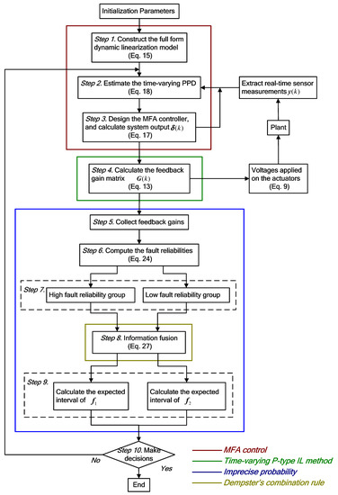
Figure 1.
Flow chart of the proposed method.
Step 1. Construct the full-form dynamic linearization model in Equation (15).
Step 2. Predict the time-varying PPD values in Equation (18) merely using the on-line system input and output data.
Step 3. Design the MFA controller in Equation (17).
Step 4. Calculate the feedback gain matrix in Equation (13).
Step 5. Extract real-time feedback gains used to transfer the characteristic parameters .
Step 6. Calculate the fault reliabilities in Equation (24) for all sensors.
Step 7. Divide the fault reliability value vector into two groups: the high fault reliability group and the low fault reliability group Equation (25).
Step 8. Respectively fuse the elements of the two groups above using Dempster’s combination rule Equation (27).
Step 9. Establish the fault probability interval by the fused results and calculate the expected interval Equation (30) of the diagnoses cost function Equation (29).
Step 10. Make decisions based on the lower expected utility and stopping criteria.
6. Numerical Simulations
6.1. FE Modeling and Setting of Controller Parameters
The numerical simulations were carried out via vibration active control on the cantilevered plate with piezoelectric patches. The piezoelectric cantilevered plate comprise done laminated composite plate (414 mm × 120 mm × 1 mm), on which six piezoelectric patches (60 mm × 24 mm × 1 mm) were bonded in pairs at the plate, as shown in Figure 2. The laminated composite plate was made of graphite-epoxy (GE, carbon-fiber reinforced) composite material, which included five substrate layers. Its total thicknesswas1mm with the angle-ply (0/90/0/90/0), and the thickness of each substrate was 0.2 mm. The upper piezoelectric patches were actuators and the lowers ones worked as sensors. We distinguished the three actuator–sensor pairs as a, b and c, respectively. The positions of the piezoelectric patches were chosen via Reference [29]. The locations of Point A, Point B and Point C are given in Figure 2. The root of the laminated composite plate was clamped. The properties of the laminated composite plate and piezoelectric material are listed in Table 1.
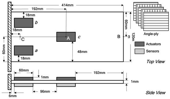
Figure 2.
The piezoelectric cantilevered plate.

Table 1.
Material properties.
In this paper, the dynamic FE model for simulating the piezoelectric cantilevered plate was constructed using ANSYS. The laminated composite plate and piezoelectric patches were modeled by SOLID46 elements and SOLID5 elements, respectively. The laminated composite plate was meshed with 69 × 20 × 1 elements, and each piezoelectric patch was meshed with10 × 4× 1 elements. For the degree of electric freedom, the nodes at the surface of piezoelectric patches were coupled by command . Modal analysis was carried out to identify the natural frequencies of the piezoelectric cantilevered plate and to design the sampling period for the numerical simulations [30]. The first three natural frequencies of the piezoelectric cantilevered plate were calculated, which also implied good agreement with the comparison between the numerical results and experimental results in Table 2. The largest error percentage, 13.9%, arose in the second modal frequency. Since the numerical results of the modal frequencies were used to get approximate values to verify the dynamic FE model, the difference in the modal frequencies between the numerical and experimental results were acceptable. The sampling period was taken as , where represented the first natural frequency of the piezoelectric cantilevered plate. were the Rayleigh damping coefficients.
Table 2.
The results of natural frequencies.
The constants of the MFA controllers were given as: , , , and . The fault reliability can be calculated in Equation (24). The system in this paper consisted of two types of states: learning termination and normal learning. The square root values of the feedback gains were regarded as the characteristic parameters. The constants for the calculation of the basic fault reliability assignment Equation (23) are given as: , , and . The constants of the diagnosis cost functions are defined as: , , ,and . The threshold value is predefined to serve as the stopping criteria, and decision-making can be fulfilled by comparing with the threshold value. The controllers connected with different sensors may have distinct convergence speeds. To make all controllers sufficiently learn, two threshold values were defined as: for the lower expected utility of fused fault reliabilities, the threshold value was specified at 0.9323; for the single fault reliability, the threshold value was specified at 0.7978. The learning process should be terminated as long as one of the two threshold values above was met. Otherwise, the learning process should be continued. In the P-type IL method, the maximum iteration number was defined as 500, and the fixed learning gains were given as and for various simulations.
6.2. Harmonic Excitation
The vibration active control for the first mode of the piezoelectric cantilevered plate was investigated in this case. Considering the harmonic excitation generated by the function , the plate was driven at Point C, the constant (5.4377Hz) was the first natural frequency. All numerical results corresponding to the robust MFA-IL control are also given in this section.
In Figure 3a,b, the time-history dynamic responses at Point A and Point B are, respectively, given, and the figure illustrates that the first mode vibration was suppressed effectively by the proposed method, the P-type IL method and robust MFA-IL control. The control performance of the piezoelectric actuators was not able at the places with (e.g., Point A) or without piezoelectric sensors (e.g., Point B). Nevertheless, it is worth noting that the conclusions obtained above were distinct from Saleh′s [31]. Saleh pointed out that the P-type IL method cannot effectively control the unwanted vibration at locations of the observation points. Furthermore, it was also noteworthy that the P-type IL method could not obviously control the first mode vibration of the piezoelectric structures.
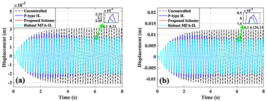
Figure 3.
Displacement responses to harmonic excitation: (a) Point A, (b) Point B.
As an effective vibration active control system, it is possible to reduce the amplitude of the overall structure not merely the parts of the structure. Before designing the vibration active control system, the control rule needs to be considered carefully for achieving satisfactory control results. The control performance of the system also relates to the positions and sizes of the piezoelectric patches [32]. The best positions for the piezoelectric patches were always chosen at the places where the mechanical strain was the largest. To generate satisfactory control forces, the dimensions of the piezoelectric actuators should be investigated and designed. The dimensions of the piezoelectric sensors should be selected appropriately, and then precise information on the structural vibration can be acquired. A misreading of sensor measurement signals may generate unreasonable control force, and the dynamic performance of the system may seriously deteriorate. As long as the positions and dimensions of the piezoelectric patches were chosen appropriately, the P-type IL method presented good performance on the first mode vibration control. Besides, the controllability of structural vibration was notable at the locations with sensors and without sensors.
The actuator time-history voltages are presented in Figure 4a,b, and the actuator voltages changed suddenly at 4.4s while the system was controlled by the P-type IL method. After the learning processes were terminated, the amplitudes of the actuator voltages reconstructed smoothness. The controllers connected with distinct sensors had different convergence speeds in the learning processes, which may cause the control force to mismatch among each other. If a piezoelectric actuator cannot perform as desired, the adjacent piezoelectric actuators will be negatively affected. To avoid this phenomenon, more iterations are needed to improve the control stability. Less iteration numbers may directly lead to system spillover. The instability phenomenon did not occur when the system was controlled by the proposed method and the robust MFA-IL control. The measurement signals from sensor a/b and sensor c are shown in Figure 4c,d. In comparison with the P-type IL method, smaller amplitudes were obtained as long as the piezoelectric cantilevered plate was controlled by the robust MFA-IL control and the proposed method. The root mean square (RMS) values of the dynamic responses and measurement signals were used to quantitatively analyze the performance of the P-type IL method, the robust MFA-IL control, and the proposed method, which are listed in Table 3. From Table 3, both the robust MFA-IL control and the proposed method had better control performance by comparing the P-type IL method. The vibration amplitude was reduced 41.22% under the control of the proposed method, and the vibration amplitudes reduced 40.36% under the control of the robust MFA-IL control. The proposed method and the robust MFA-IL had similar control precision.
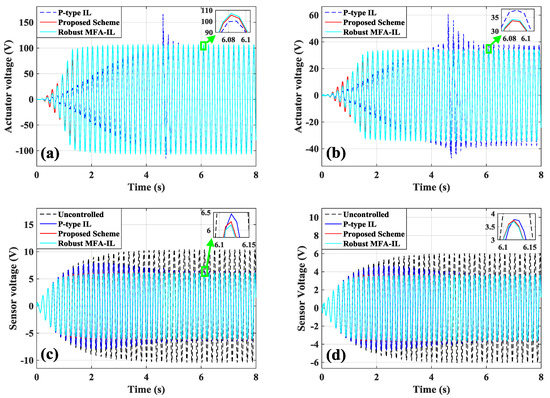
Figure 4.
The time-domain measurement signals of the actuators/sensors: (a) actuator a/b; (b) actuator c; (c) sensor a/b; (d) sensor c.
Table 3.
Root mean square (RMS) results.
The computational time for the various algorithms is shown in Figure 5, including the time for running each iteration and the time for convergence of the feedback gains. From Figure 5, both the robust MFA-IL and the proposed method have fast convergence speed, which makes them overcome the inherent shortcoming of the P-type IL method. By comparing with the proposed method, the computational burden of the robust MFA-IL control was higher when the controller implemented each iteration. The extension of computational time resulted in increasing the time delay. Large time delays will bring uncontrollability to the vibration suppression system. In the proposed method, the main computational cost focused on the part of the MFA control, which was implemented by iterative computation for determining the learning gains in real time. Apart from the MFA control, the SMC was also integrated into the robust MFA-IL control. The introduction of SMC brings great computational burden, and results in great time delays. Generally speaking, the more actuator–sensor pairs bonded on the plate, the more the vibration modes of the plate which can be controlled. Therefore, the time delay also increases with the increase in pairs of actuators–sensors, which may limit the application are as for the robust MFA-IL control. To obtain a slight improvement in control precision, the robust MFA-IL control brings a larger time delay. In practical applications, the design of the vibration control system should be composed of control precision and realization of vibration suppression. The proposed method can be based on a compromise.
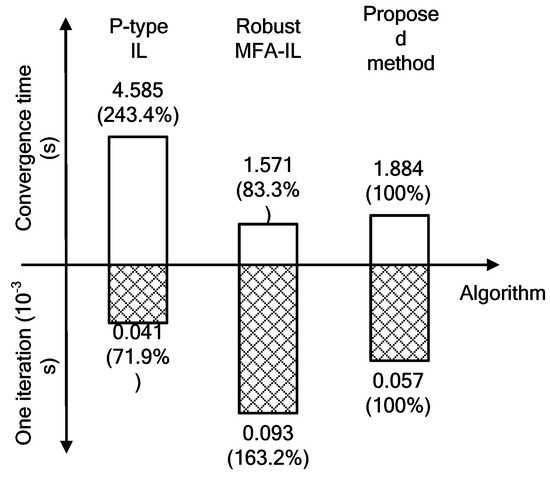
Figure 5.
The computational time for the various algorithms.
The learning processes of feedback gains are depicted in Figure 6a,b. From Figure 4 and Figure 6, the proposed method and the robust MFA-IL had fast learning speed and maintained a good control performance and system stability.
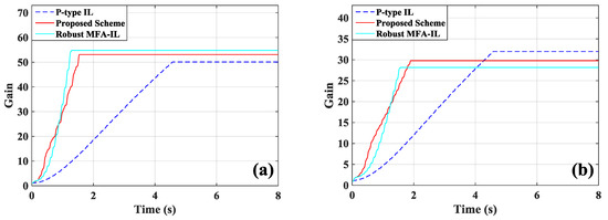
Figure 6.
The learning processes of feedback gains: (a) actuator a/b; (b) actuator c.
The real-time diagnosis results for the fused information and single information source are given in Figure 7. From Figure 7, the controllers connected with actuator a/b had faster convergence speed than that connected with actuator c. Based on the theory of imprecise probability, all controllers could learn sufficiently, and satisfactory control performance could be achieved.
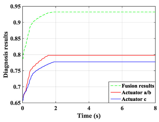
Figure 7.
The curves of diagnosis results.
To verify the stability of the controllers, an instability test is carried out in this section. The noise signals are shown in Figure 8 are added to excite the piezoelectric cantilevered plate at Point A. The noise signals start at 6s and lasts only one second. The parameters of controllers are set up the same as mentioned above. The time-history dynamic responses at Point A and Point B are given in Figure 9a, and the measurement signals from sensor a/b and sensor c are shown in Figure 9b. When noise signals begin to excite, the dynamic responses of the plate and measurement signals from sensors change greatly; however, the divergence phenomenon was not found. After stopping the excitation of the noise signals, the vibration control system was restored to the stability state by the proposed method.
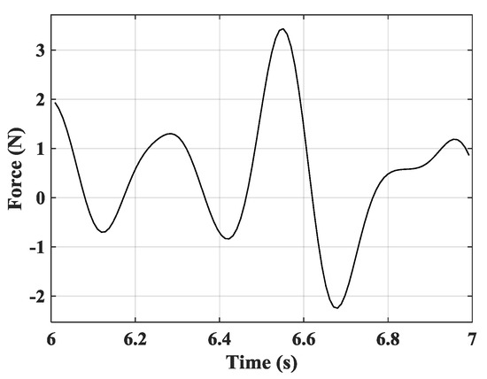
Figure 8.
The noise signals.
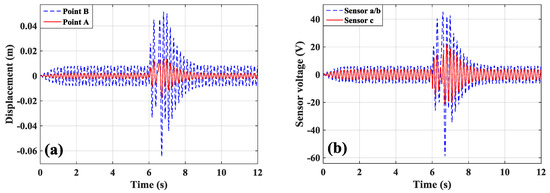
Figure 9.
Verification curves with the stability of the proposed method: (a) displacement responses and (b) measurement signals of sensors.
6.3. Random Excitation
In this case, the plate was driven at Point C by the random force as follows in Figure 10.
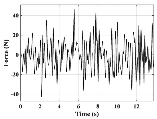
Figure 10.
The random excitation.
The time-history dynamic responses at Point A and Point B are shown in Figure 11. The control voltages of actuator a/b and actuator c are presented in Figure 12a,b. The measurement signals from sensor a/b and sensor c are displayed in Figure 12c,d. The feedback gains are depicted in Figure 13.
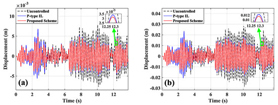
Figure 11.
Displacement responses to random excitation: (a) Point A; (b) Point B.
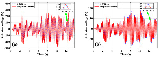
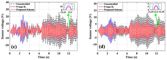
Figure 12.
The time-domain measurement signals of actuators/sensors: (a) actuator a/b; (b) actuator c; (c) sensor a/b; (d) sensor c.
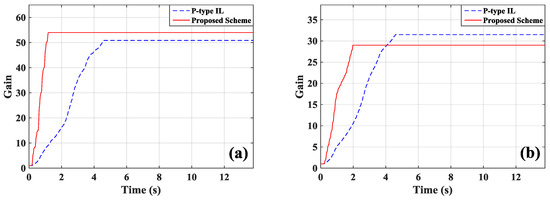
Figure 13.
The learning processes of feedback gains: (a) actuator a/b; (b) actuator c.
From the results above, the proposed method makes the system have smaller amplitudes of dynamic responses and faster convergence speed. The learning gain in P-type IL method is the fixed constant, which is selected based on the practical experience of researchers. A larger learning gain can lead to system instability and robustness reduction [10], thus, a smaller learning gain is necessary to improve the system control precision. However, the smaller the learning gain selected, the more iterations are needed, thus the learning speeds of controllers slow down [7,9]. In the proposed method, the learning gain can be self-tuned by the system’s dynamic behavior. The convergence speeds of the controllers are improved, and the high control precision can also be obtained.
In this case, the RMS values for evaluating the proposed method and the P-type IL method are listed in Table 3. The real-time diagnosis results of the system states are given in Figure 14.

Figure 14.
The curves of diagnosis results.
7. Experiments
7.1. ExperimentSetup
To validate the feasibility and control effect of the proposed method, an experimental system to control the vibration of the piezoelectric cantilevered plate was developed, as shown in Figure 15. Experiments on the first mode vibration control were conducted. The experiment setup consisted of a piezoelectric cantilevered plate with one laminated composite plate and six piezoelectric patches, the vibration excitation system, the data acquisition system, and the vibration active control system. The laminated composite plate was made up of GE composite material. The dimensions of the piezoelectric cantilevered plate are given in Section 6.1. The excitation position Point C was replaced by a metal patch.
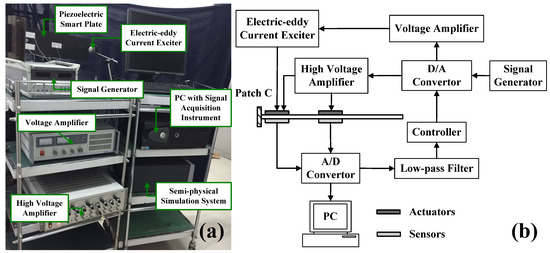
Figure 15.
Experimental setup: (a) experimental setup and (b) experimental principle.
The signal generator (DH1301, Taizhou, China) was used to generate the external excitation signals. After digital to analog (D/A) conversion, the excitation signals were amplified by the voltage amplifier (YE5872A, PA, USA) and then were used to drive the piezoelectric cantilevered plate by the electric-eddy current exciter (JZF-1, Beijing, China). The electric signals were transformed into a mechanical force. Three piezoelectric sensors were applied to detect the vibration information, and their measurement signals were selected as the feedback signals. After analog-to-digital (A/D) conversion, all measurement data were acquired and stored in the PC. Since the control target of the piezoelectric cantilevered plate was the first mode, a low-pass filter was applied to eliminate the high-frequency noise. The controllers implemented the signal processing and calculation in the real-time semi-physical simulation system (Quarc, Toronto, Canada). Running the proposed method, the controllers generated the control signals. After D/A conversion, the control outputs were sent to the high-voltage amplifier (E70, Harbin, China) and then were applied to piezoelectric actuators for vibration suppression. The experimental sample period was chosen as 3 ms.
7.2. Modal Analysis
A swept sine (chirp) signal with an amplitude of 100 V was used to identify the modal frequencies of the system and excite actuator a. The initial frequency was 0.5 Hz, and the terminal frequency was50 Hz.
Fourth-order Butterworth filters were utilized to eliminate high-frequency noises. The cutoff frequency of low-pass filters was specified at 30 Hz in the modal identification, and the cutoff frequency was14 Hz in the first mode control. After filtering, the time-domain response signal measured by sensor a was stored and shown in Figure 16a. The fast Fourier transform (FFT) of the time-domain response data was computed to depict the frequency response of the system in Figure 16b. From Figure 16b, the first three modal frequencies were obtained and are listed in Table 2.
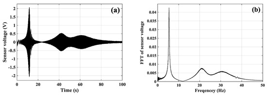
Figure 16.
Vibration responses excited by actuator a: (a) the time-domain measurement signals of the sensor a; (b) frequency response of the sensor a.
7.3. ExperimentResults
The proposed method and the P-type IL method were investigated for vibration active control of the flexible plate during the experiments. In this section, the plate was driven at 5.326 Hz for the first mode control. In the P-type IL method, the number of iterations was predefined as 1500 to improve the system stability and control precision, and the value of learning gain was specified as . In the MFA controller, the parameters were selected as , , ,and . The stopping criteria in this section were the same with those above in Section 6.1. The measurement signals of the sensors (shown in Figure 17a,b) were moved forward for the phase delay compensation due to the hardware factors. The P-type IL method and the proposed method were performed at 5 s after the harmonic excitation started.
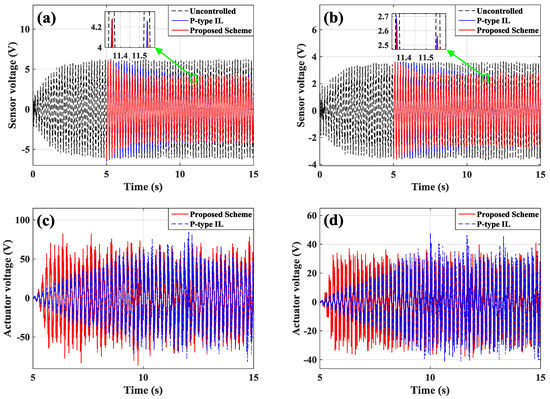
Figure 17.
The time-domain measurement signals of actuators/sensors: (a) sensor a/b; (b) sensor c; (c) actuator a/b; (d) actuator c.
The measurement signals from sensor a/b and sensor c are presented in Figure 17a,b, and the control voltages of actuator a/b and actuator c are presented in Figure 17c,d. The data used to calculate the RMSs are recorded after learning termination, and the RMSs are given in Table 3. From Table 3, the proposed method reached the comparatively ideal control performance: the vibration amplitudes were reduced 33.9% under the control of the proposed method, and the vibration amplitudes were reduced 31.8% under the control of the P-type IL method. This excellent performance was obtained by integrating the MFA method into time-varying P-type IL method. The learning processes of the feedback gains are depicted in Figure 18. The proposed method is feasible to simultaneous maintain the control performance and damp down quickly for structural vibration. Under the control of different methods, the feedback gains obtained from the same controllers result in distinct values. The real-time diagnosis curves for the fused information and single information sources are given in Figure 19. By the theory of imprecise probability, the learning processes of feedback gains can be diagnosed in real time. The decisions made based on the designed stopping criteria causes all controllers to learn sufficiently, and excellent control performance was obtained.
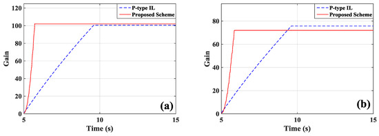
Figure 18.
The learning processes of feedback gains: (a) actuator a/b; (b) actuator c.
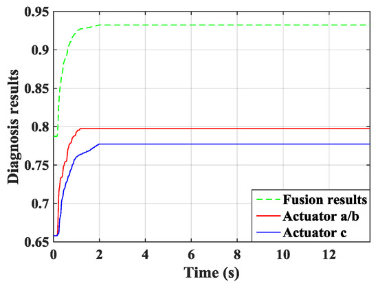
Figure 19.
The curves of the diagnosis results.
8. Conclusions and Outlooks
A data-driven adaptive IL method was proposed for vibration active control of piezoelectric laminated composite structures. Based on the P-type IL method, the motion equation of the piezoelectric cantilevered plate was derived by the dynamic FE equations. The PPD matrix is estimated by the modified projection algorithm for dynamically linearizing the motion equation. Considering the uncertain non-linear dynamic processes, the MFA controller was designed. The MFA method was applied to self-tune the learning gains of the time-vary P-type IL method for accelerating the learning speed. The square root values of the feedback gains were regarded as characteristic parameters to diagnose the state of the vibration control system. Based on the theory of imprecise probability, the stopping criteria were designed. On this basis, the decisions were carried out to avoid the over-learning of controllers.
When the positions and dimensions of the piezoelectric patches are chosen appropriately, the P-type IL method shows good effectiveness on the first mode control of the piezoelectric cantilevered plate. Besides, the good controllability of the structural vibration was notable at the locations with sensors or without sensors. The conclusions obtained above in this paper were different other published studies.
Considering the system uncertainties, the MFA method was applied to self-tune in real-time the learning gains by the system’s dynamic behavior. The introduction of the MFA method accelerated the convergence speed of the controller and improved the system’s control precision. The stopping criteria based on the theory of imprecise probability allowed all controllers to learn sufficiently, and satisfactory control performance was achieved. The proposed method overcomes the shortcomings of the P-type IL method to achieve the expected control performance. The robust MFA-IL control improved control precision at the expense of great time delay, while the proposed method reduced the computational burden and misdiagnosis for system states at the expense of a slight decrease in control precision. The proposed method in this paper can be a compromise.
The proposed method has an open scheme, which can be integrated with other methods, including a model-based method. The data-driven method and model-based method can be complementary and cooperative in the design of a control system. The more precise information and model of the system obtained, the better the control performance of the system can be expected. In the future, the proposed method can be integrated with a model identification method to handle more complex problems in practical applications, which will simplify the structure of controllers and obtain a satisfactory control precision.
Author Contributions
Conceptualization, L.B.; Methodology, L.B.; Software, L.B.; Validation, X.-F.X., N.L. and Y.C.; Formal Analysis, L.B.; Investigation, L.B. and Y.C.; Resources, Y.-W.F.; Data Curation, L.B. and X.-F.X.
Funding
The research was funded by National Natural Science Foundation of China under Grant No. 5187051969.
Acknowledgments
All authors thank the editors, referees and officers in Symmetry for their valuable suggestions and help.
Conflicts of Interest
The authors declare no conflicts of interest.
References
- Ruan, X.; Bien, Z.Z.; Wang, Q. Convergence characteristic of proportional-type iterative learning control in the sense of Lebesgue-p norm. IET Control Theory A 2012, 6, 707–714. [Google Scholar] [CrossRef]
- Ajjanaromvat, N.; Parnichkun, M. Trajectory tracking using online learning LQR with adaptive learning control of a leg-exoskeleton for disorder gait rehabilitation. Mechatronics 2018, 51, 85–96. [Google Scholar] [CrossRef]
- Xu, J.X.; Huang, D.Q.; Venkatakrisham, V.; Tuong, H. Research on flexible dynamics of a 6-DOF industrial robot and residual vibration control with a pre-adaptive input shaper. J. Mech. Sci. Tecnol. 2019, 33, 1875–1889. [Google Scholar]
- Cao, Z.X.; Zhang, R.D.; Yang, Y.; Lu, J.Y.; Gao, F.R. Iterative learning control and initial value estimation for probe-drogue autonomous aerial refueling of UAVs. Aerosp. Sci. Technol. 2018, 82–83, 583–593. [Google Scholar]
- Freeman, C.T.; Tan, Y. Iterative learning control with mixed constraints for point-to-point tracking. Defence Technol. 2017, 13, 360–366. [Google Scholar]
- Zhu, X.J.; Gao, Z.Y.; Huang, Q.Z.; Yi, J.C. ILC based active vibration control of smart structures. IEEE Int. Conf.Intell. Comput.Intell. Syst. 2009, 2, 236–240. [Google Scholar]
- Tavakolpour, A.R.; Mailah, M.; Intan, Z.; Darus, M.; Tokhi, O. Self-learning active vibration control of a flexible plate structure with piezoelectric actuator. Simul. Model Pract. Theory 2010, 18, 516–532. [Google Scholar] [CrossRef]
- Zhang, Y.L.; Xu, Q.S. Adaptive iterative learning control combined with discrete-time sliding mode control for piezoelectric nanopositioning. In Proceedings of the 35th Chinese Control Conference, Chengdu, China, 27–29 July 2016; pp. 6080–6085. [Google Scholar]
- Xu, J.X.; Wang, W.; Huang, D.Q. Iterative learning in ballistic control. In Proceedings of the 2007 American Control Conference, New York, NY, USA, 11–13 July 2007; pp. 1293–1298. [Google Scholar]
- Tan, Y.; Dai, H.H.; Huang, D.Q.; Xu, J.X. Unified iterative learning control schemes for nonlinear dynamic systems with nonlinear input uncertainties. Automatica 2012, 48, 3173–3182. [Google Scholar] [CrossRef]
- Taher, A.; Marwan, A.; Binish, J. Wavelets approach for the optimal control of vibrating plates by piezoelectric patches. J. Vib. Control 2018, 24, 1101–1108. [Google Scholar]
- Qiu, Z.C.; Zhang, X.T.; Zhang, X.M.; Han, J.D. A vision-based vibration sensing and active control for a piezoelectric flexible cantilever plate. J. Vib. Control 2016, 22, 1320–1337. [Google Scholar] [CrossRef]
- Li, S.Q.; Li, J.; Mo, Y.P. Piezoelectric multimode vibration control for stiffened plate using ADRC-based acceleration compensation. IEEE Trans. Ind. Electron. 2014, 61, 6892–6902. [Google Scholar] [CrossRef]
- Lim, Y.H. Finite-element simulation of closed loop vibration control of a smart plate under transient loading. Smart Mater. Struct. 2003, 12, 272–286. [Google Scholar] [CrossRef]
- Hou, Z.S.; Wang, Z. From model-based control to data-driven control: Survey, classification and perspective. Inform. Sci. 2013, 235, 3–35. [Google Scholar] [CrossRef]
- Hou, Z.S.; Chi, R.H.; Gao, H.J. An overview of dynamic-linearization-based data-driven control applications. IEEE Trans. Ind. Electron. 2017, 64, 4076–4089. [Google Scholar] [CrossRef]
- Wang, Z.S.; He, D.K.; Zhu, X.; Luo, J.H.; Liang, Y.; Wang, X. Data-driven model-free adaptive control of particle quality in drug development phase of spray fluidized-bed granulation process. Complexity 2017, 4960106. [Google Scholar] [CrossRef]
- Bu, X.H.; Cui, L.Z.; Hou, Z.S.; Qian, W. Formation control for a class of nonlinear multiagent systems using model-free adaptive iterative learning. Int. J. Robust. Nonlinear Control 2018, 28, 1402–1412. [Google Scholar] [CrossRef]
- Chi, R.H.; Hou, Z.S. Dual stage optimal iterative learning control for nonlinear non-affine discrete-time system. ActaAutom. Sin. 2007, 33, 1061–1065. [Google Scholar] [CrossRef]
- Bai, L.; Feng, Y.W.; Li, N.; Xue, X.F. Robust model-free adaptive iterative learning control for vibration suppression based on evidential reasoning. Micromachines 2019, 10, 196. [Google Scholar] [CrossRef]
- Jiang, W. A correlation coefficient for belief functions. Int. J Approx. Reason. 2018, 103, 94–106. [Google Scholar] [CrossRef]
- Lu, C.Q.; Wang, S.P.; Wang, X.J. A multi-source information fusion fault diagnosis for aviation hydraulic pump based on the new evidence similarity distance. Aerosp. Sci. Technol. 2017, 71, 392–401. [Google Scholar] [CrossRef]
- Hable, R. Data-based decisions under imprecise probability and least favorable models. Int. J. Approx. Reason. 2009, 50, 642–654. [Google Scholar] [CrossRef][Green Version]
- Destercke, S. A k-nearest neighbors method based on imprecise probability. Soft Comput. 2012, 16, 833–844. [Google Scholar] [CrossRef]
- Tien, S.C.; Zou, Q.Z.; Devasia, S. Iterative control of dynamics-coupling-caused errors in piezoscanners during high-speed AFM operation. IEEE T. Contr. Syst. T. 2005, 13, 921–931. [Google Scholar] [CrossRef]
- Matthias, C.M.T. Decision making under uncertainty using imprecise probability. Int. J. Approx. Reason. 2007, 47, 17–29. [Google Scholar]
- Razi, S.; Mollaei, M.R.K.M.; Ghasemi, J. A novel method for classification of BCI multi-class motor imagery task based on Dempster-Shafer theory. Inform. Sci. 2019, 484, 14–26. [Google Scholar] [CrossRef]
- Dong, X.J.; Peng, Z.K.; Ye, L.; Hua, H.X.; Meng, G. Performance evaluation of vibration controller for piezoelectric smart structures in finite element environment. J.Vib. Control. 2014, 20, 2146–2161. [Google Scholar] [CrossRef]
- An, J.Y.; Hu, M.; Fu, L.; Zhan, J.W. A novel fuzzy approach for combining uncertain conflict evidences in the Dempster-Shafer theory. IEEE Access. 2018, 7, 7481–7501. [Google Scholar] [CrossRef]
- Malgaca, L. Integration of active vibration control methods with finite element models of smart laminated composite structures. Compos.Struct. 2010, 92, 1651–1663. [Google Scholar] [CrossRef]
- Saleh, A.R.T.; Mailah, M. Control of resonance phenomenon in flexible structures via active support. J Sound Vib. 2012, 331, 3451–3465. [Google Scholar] [CrossRef]
- Nemanja, D.Z.; Aleksandar, M.S.; Zoran, S.M.; Slobodan, N.S. Optimal vibration control of smart composite beams with optimal size and location of piezoelectric sensing and actuation. J. Intell. Mat. Syst. Struct. 2012, 24, 499–526. [Google Scholar]
© 2019 by the authors. Licensee MDPI, Basel, Switzerland. This article is an open access article distributed under the terms and conditions of the Creative Commons Attribution (CC BY) license (http://creativecommons.org/licenses/by/4.0/).