A Unified Multiple-Phase Fluids Framework Using Asymmetric Surface Extraction and the Modified Density Model

Abstract

Multiple-phase fluids’ simulation and 3D visualization comprise an important cooperative visualization subject between fluid dynamics and computer animation. Interactions between different fluids have been widely studied in both physics and computer graphics. To further the study in both areas, cooperative research has been carried out; hence, a more authentic fluid simulation method is required. The key to a better multiphase fluid simulation result is surface extraction. Previous works usually have problems in extracting surfaces with unnatural fluctuations or detail missing. Gaps between different phases also hinder the reality of simulation. In this paper, we propose a unified surface extraction approach integrated with a modified density model for the particle-based multiphase fluid simulation. We refine the original asymmetric smoothing kernel used in the color field and address a binary tree scheme for surface extraction. Besides, we employ a multiphase fluid framework with modified density to eliminate density deviation between different fluids. With the methods mentioned above, our approach can effectively reconstruct the fluid surface for particle-based multiphase fluid simulation. It can also resolve the issue of overlaps and gaps between different fluids, which has widely existed in former methods for a long time. The experiments carried out in this paper show that our approach is able to have an ideal fluid surface condition and have good interaction effects.

1. Introduction

Visualized fluid simulation has been studied for a long time and with the help of both fluid dynamics and computer animation techniques. There have been various kinds of methods for fluid simulation visualization. They can be divided into two types based on the difference of the spatial discretization method, which are mesh-based Euler approaches and particle-based Lagrangian approaches. In Euler approaches, the simulation domain is discretized into mesh grids, and the physical values on grid points (such as acceleration, pressure) can be obtained through the governing equations. Mesh-based methods can create animations with a realistic appearance, but they are time-consuming and have difficulty handling certain phenomena accurately like free surfaces, complex boundaries, and splashes. Nevertheless, in particle-based methods like the Smoothed Particle Hydrodynamics (SPH), the volume of the fluid is discretized by particles. Each of them carries physical properties and moves freely according to the velocity field. Particle-based methods can easily maintain momentum conservation and incompressibility and have been used to simulate various kinds of phenomena, such as water, smoke, deformable solids, as well as viscoelastic liquids and multiphase fluids. However, some major particle-based methods have difficulties in producing realistic surfaces, especially for multiphase interactions.

In daily life, multiphase phenomena like water bubbles and the mixture of immiscible fluids are everywhere. Currently, multiphase simulation is receiving wide attention. While in SPH simulation, there is a certain spatial distance between particles and particles’ properties are smoothed by the kernel function, when the static density and mass of neighbor particles are different, the physical quantity calculated using SPH approach will be biased. This problem is especially obvious at the interface of multiple phases. The density value calculated by the fluid with high static density near the interface is relatively small, while the density value calculated by the fluid with low static density is relatively large. This is because the standard SPH formula smooths the density at the interface and does not accurately represent a sharp change in density. Moreover, due to the density deviation, the calculation deviation of other physical quantities, such as pressure, will lead to unreal interface effects and serious numerical instability. Besides, extracting high-quality surfaces of multiple phases from particle locations has been rarely discussed. The standard approaches for reconstructing surfaces of particle-based simulation usually need to create an implicit surface, which virtually wraps around all the particles during the simulation. Although recent research has significantly improved the surface appearance that results from formulating the implicit function, unfortunately, there have still been problems for these methods in accurately and stably handling interface evolutions, especially at the location where the multiphase interface lies. Few research works have focused on the problem of extracting smooth surfaces and the interface in multiphase simulation for particles.

In this paper, we present a novel surface extraction approach integrated with the multiphase model with modified density, which significantly improves the appearance at the multiphase interface while keeping a good fluid surface quality. We employ an asymmetric smoothing kernel to represent each particle. The direction and scale of the asymmetry are determined by the distribution of the particle’s neighborhood. The asymmetric kernel is constructed like Yu’s [1] method, but we consider the influence of other phases when computing one phase’s kernel and color field. Besides, we also address a binary tree strategy [2], which is convenient to implement to divide equally the overlap area and fill up the vacuum space. In addition, we employ a multiphase fluids model to eliminate density deviations at the interface. The results show that our method acquires a better realistic appearance of the fluid surface and interface when compared to previous methods. More importantly, the binary tree strategy can suit the data-driven approach easily to further boost the process, which shows great potential in surface-specified enhancement that would be a promising topic for 3D visualization of fluids.

2. Related Work

Currently, SPH is a popular approach for fluid simulation. Desbrun [3] started to simulate deformable objects with SPH. Monaghan [4] addressed free surface flow simulation approaches with SPH as a basis for fluid simulation. Later, Müller et al. [5] firstly applied SPH in computer graphics for fluid simulation. They employed Boyle’s law and surface tension, as well as viscosity forces to calculate forces, which brought the problem of compressibility. Based on the former studies, Becker and Teschner [6] proposed Weakly-Compressible SPH (WCSPH) using the Tait equation. This method reduced compressibility significantly and increased the fidelity; however, the efficiency of simulation was limited severely by the time step. A more strict incompressibility condition would require smaller time steps, which cost much more time for computation. After that, more advanced approaches were proposed to improve the fidelity and efficiency. Solenthaler and Pajarola [7] presented the Predictive-Corrective Incompressible SPH (PCISPH) method that uses a prediction-correction scheme to determine the particle’s pressure. PCISPH can increase time steps remarkably, making it more efficient than WCSPH. He et al. [8] presented a similar method, Local Poisson SPH (LPSPH), which can ensure incompressibility by an iterative process. Afterwards, Ihmsen et al. [9] addressed Implicit Incompressible SPH (IISPH). This method builds the Pressure Poisson Equation (PPE) carefully and then solves the linear problem with the relaxed Jacobi approach. This method has a great improvement in both stability and convergence speed. Particularly, IISPH is especially fit for large-scale simulation. Recently, an approach with potential for SPH fluid simulation was introduced by Bender and Koschier [10]. It combines two pressure solvers together to restrict low volume compression and ensure a divergence-free velocity field. What is more, this method is able to carry out the simulation in large time steps, yet enhancing the appearance.

For the density deviation of the SPH formula at the interface, Hoover [11] firstly described the problem of false interfacial tension caused by small particle density and pressure calculation near the interface. Agertz et al. [12] also presented a similar situation, pointing out that the wrong pressure would create voids and severe instability between two-phase fluids with a high density ratio. In order to deal with the numerical instability problem caused by the increase of the density ratio, Ott et al. [13] proposed an improved continuity equation. Although it is very effective for some special application scenarios, neither the standard nor improved continuity equation can produce stable long-term simulation results. This can lead to serious density integral errors, especially when using large time steps and low order time integral schemes. Tartakovsky et al. [14] proposed a corrected formula for density summation, which combined the corrected SPH flow equation with the advection diffusion equation to simulate the miscible flow with complex geometry. Hu et al. [15] focused on the study of numerical examples of droplet oscillation and deformation in two-dimensional shear flow. In addition, early studies on multiphase fluids included solving a discontinuous interface [16,17,18] and focusing on bubble and foam [19,20,21], which are all based on the Euler method. Losasso et al. [22] proposed a level set method that uses SPH particles to represent diffusion regions, and Thurey et al. [23] proposed a foam simulation method based on SPH. Muller et al. [24] proposed an SPH-based particle simulation method to deal with multiphase and water boiling. Mao et al. [25] simulated immiscible fluid by explicitly detecting collision particles. Solenthaler et al. [26] used quantitative density to improve density summation and employed it to correct other physical quantities to solve the problem of the false interface effect.

Particle-based fluid simulation has difficulty with surface extraction, for those particles cannot give any interrelated information. In the past several decades, researchers have addressed several surface extraction methods for particle-based fluid simulation. Blinn presented the blobby sphere approach [27], which computes the distance between the scattered points and sampling points as a parameter to accumulate the implicit surface functions. It successfully reconstructs surfaces from discrete points, but whether the density of the particles is high or low, they would always cause indentations or become bumpy on the surface. Müller et al. [5] introduced a color field approach as a kind of level set scheme to construct the fluid surface simply and rapidly. However, the surface being extracted was rough, and bumps were produced by particles next to the surface. Zhu and Bridson improved the blobby sphere approach by adjusting density variations of the local particles [28]. They first calculated the fluid particles’ radius, as well as the coordinates’ weighted mean according to the neighbor particles’ radius and position. Then, the weighted mean radius and coordinates were used to extract surfaces that became a relatively smoothed fluid surface compared to the original blobby sphere approach. Adams et al. [29] modified Zhu’s approach through tracking the distances between the particle and surface over time. This method can successfully produce smooth surfaces for both fixed radius and adaptive particles with the cost of excessive time. Bhatacharya et al. [30] introduced a level set approach considering surface reconstruction as an optimization issue. To obtain a smooth surface, they smoothed the initial surfaces through an iteration process. Yu et al. [31] introduced an alternate approach. They built the surfaces only at the beginning of the simulation, which reduced the computation cost. Akinci et al. [32] introduced a scheme to reconstruct and optimize the surface concurrently and presented a surface tectonic line approach [33]. Yu and Turk [1] presented the implicit surface with asymmetric kernels, which are able to extract smoother fluid surfaces with more fidelity. In their approach, a unique kernel function was applied for each particle, which was constructed according to the distribution of the neighbors of the particles. It can handle planar fluid so easily that even thin surfaces with sharp features are still able to achieve an ideal appearance.

Furthermore, Because the topology changes and movements of the multiphase interface are quite complicated, it is a very challenging issue to track the multiphase interface. The multiphase interface always plays an important role in the multiphase simulation. In the past few years, researchers have proposed many methods for multiphase interface tracking. Level set methods [34] often replace the binary sign of the distance field with an integer phase label to extend to multiphase interface tracking [21,35,36,37]. In a number of methods, one signed distance field is used for each phase, while other methods used a single unsigned distance field for all phases to reduce memory and computation costs. Starinshak et al. [38] presented an issue about multiple level set methods, i.e., overlaps or voids at the triple phase interface, which is usually corrected through projection. Da et al. [39] explicitly tracked such a triple phase interface that avoided vacuums and overlaps by reconstruction. Volume-of-fluid methods [40] allocate a volume fraction for each cell, and their multiphase material stores a partition of unity, i.e., one fraction each phase. Then, this information is used to reconstruct a continuous multiphase interface [41,42]. Moving mesh or semi-Lagrangian methods [43,44,45,46,47] allot phase labels to each volume element. Some recent research discussed the issue of mesh maintenance [48,49]. Particle-based surface reconstruction augments each particle with a phase label or color [24,26] or allocates phase attributes to particles directly.

However, most of these methods cannot be directly integrated with particle-based fluid simulation, and this existing method is difficult to achieve. In addition, the surface and interface appearance of the reconstructed fluid are pretty rough with gaps or overlaps. Therefore, we introduce a much easier method to build the multiphase interface by applying asymmetric kernels, which can eliminate the overlaps and gaps of the multiphase interface in surface reconstruction.

3. SPH Fluid Simulation

SPH has become a popular approach for interpolation in Lagrangian systems. The main idea of the SPH method is to represent continuous fields using discrete particles and apply the integral to approximate the field. A scalar quantity $A\left(x_i\right)$ of particle i at location $x_i$ can be interpolated by the sum of quantities from neighbor particles in the Standard SPH (SSPH) method:

$$〈A\left(x_i\right)〉=\sum _j^{}{m}_j\frac{A_j}{{\rho }_j}W\left(x_i-x_j,h\right)$$

(1)

where $m_j$ and ${\rho }_j$ represent the mass and density of each particle, $W\left(x_i-x_j,h\right)$ is the smoothing kernel used in the SPH approach, and h is the smoothing length.

In the SPH method, the Navier–Stokes equation is discretized based on particle locations, which can be written as a differential equation as follows:

$${\rho }_i\frac{\partial {\mathbf{v}}_i}{\partial t}=-〈\nabla p_i〉+\mu 〈{\nabla }^2{\mathbf{v}}_i〉+{\mathbf{f}}_i^{ext}$$

(2)

where ${\mathbf{f}}_i^{ext}$ is the external force and $〈\nabla p_i〉$ and $〈{\nabla }^2{\mathbf{v}}_i〉$ are the pressure gradient and Laplacian form of velocity. Since the volume of fluid is represented by particles in the SPH method, the density ${\rho }_j$ can be interpolated using a weighted sum of the mass $m_j$ from neighbor particles. In order to simulate fluid using particles:

$${\rho }_i=\sum _j^{}{m}_{j}W\left(x_i-x_j,h\right)$$

(3)

$p_i$ is the pressure of each particle i, which can be calculated by the function of density. The SSPH method uses the ideal gas equation: $p_i=k({\rho }_i-{\rho }_0)$, where ${\rho }_0$ is the rest density and k is a constant determined by the researchers for different effects. Becker and Teschner [6] used the Tait equation to replace the gas equation. This can further restrict the density variations and enhance the efficiency:

$$p_i=\frac{{\rho }_0{c}_S^2}{\gamma }\left({\left(\frac{{\rho }_i}{{\rho }_0}\right)}^{\gamma }-1\right)$$

(4)

where $c_s$ is the numerical speed of sound and $\gamma$ is the stiffness parameters; we set it to seven in our experiments.

Then, pressure force ${\mathbf{f}}_i^p$ and viscous force ${\mathbf{f}}_i^{\mathbf{v}}$ between particles can be represented as:

$${\mathbf{f}}_i^p=-\sum _j^{}{m}_j(\frac{p_i}{{\rho }_i^2}+\frac{p_j}{{\rho }_j^2})\nabla W_{ij}$$

(5)

Because the second derivative of the kernel function would lead to severe numerical error and instability, we applied the artificial viscosity in this paper, so the viscous force ${\mathbf{f}}_i^{\mathbf{v}}$ is expressed as:

$${\mathbf{f}}_i^{\mathrm{v}}=2\mu (d+2)\sum _j\frac{m_j}{{\rho }_i}\frac{{\mathbf{v}}_{ij}·{\mathbf{x}}_{ij}}{|{{\mathbf{v}}_{ij}}^2|+0.01h^2}\nabla W_{ij}$$

(6)

where d is the dimension, ${\mathbf{v}}_{ij}$ and ${\mathbf{x}}_{ij}$ is the velocity and distance between two particles, and $\mu$ is the viscosity coefficient.

4. Multiple-Phase Fluids’ Simulation Using Modified Density

When different fluids are blended, whether they will mix with each other is based on the intermolecular interaction. There will be distinct multiphase interactions when they are immiscible. As shown in Figure 1, there are three phases in the whole domain. When applying the particle-based approach, there is interaction force between particles. The force between particles is equal in all directions and maintains a balance in the same phase. However, when the different phases are in touch and mix with other phases at the junction, the forces between particles are no longer balanced. Interfacial tension would emerge at the multiphase interface, which is the surface contraction force acting perpendicular to the fluid surface along the multiphase interface. The interfacial tension is similar to the surface tension effect between the fluid and the air interface, but the surface tension usually ignores the effects from gases. The interfacial tension of multiphase flow has to consider the influence of the particles of other phases; therefore, it is more complex to handle.

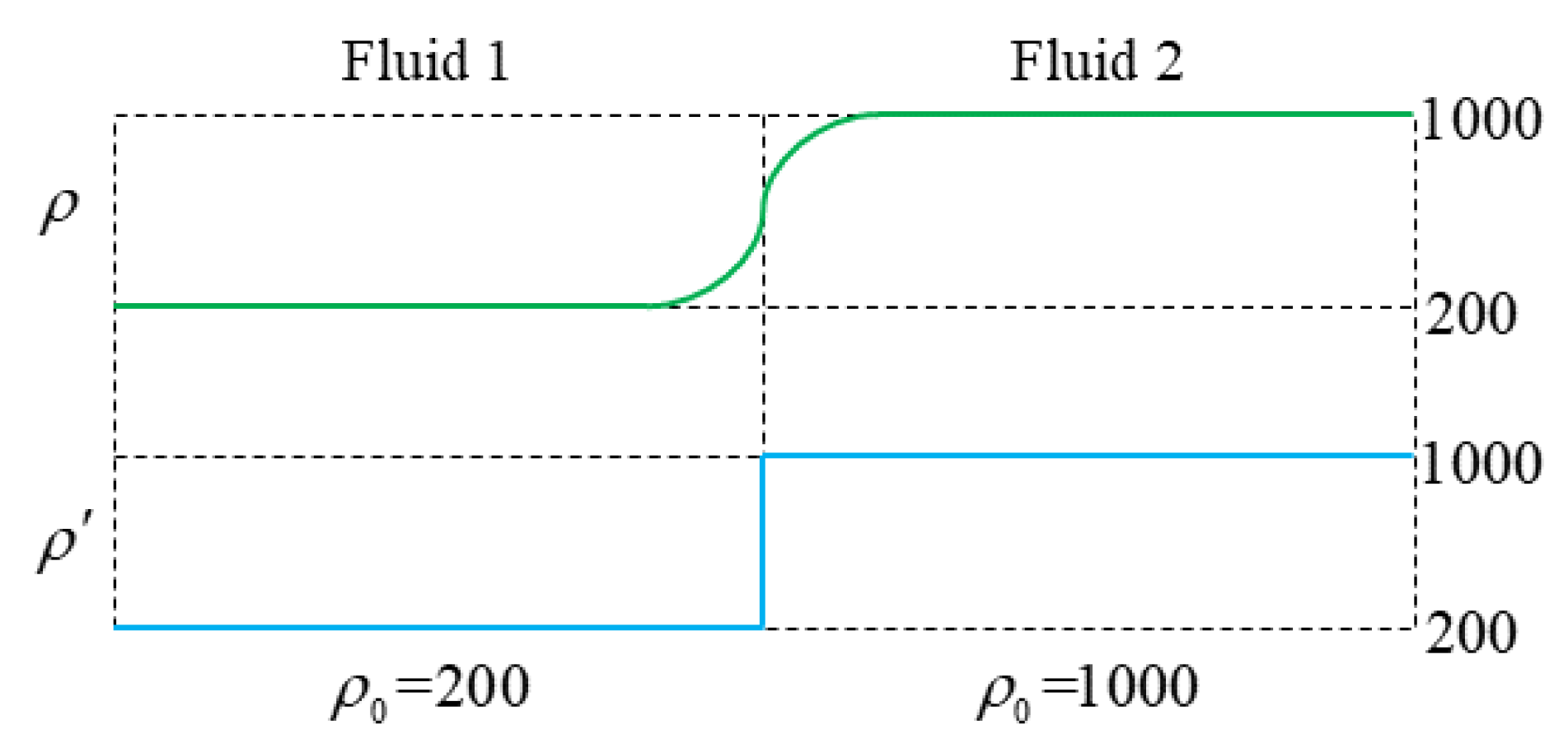
4.1. Modified Density Model

In order to deal with the density discontinuity at the multiphase interface, we applied the quantity density of Solenthaler [26] to modify the traditional formula of SPH for calculating density. The main concept of this method is that when each particle’s density is calculated according to its neighbor particles’ density, let the neighbor particles and the particle itself seem to have the same static density and mass. The quantity density ${\delta }_i$ can be written as:

$${\delta }_i=\sum _{j}W\left(x_i-x_j,h\right)$$

(7)

Construct the modified particle density ${\rho }_i^{\prime }$ as the quantity density multiplied by the current particle mass, which is:

$${\rho }_i^{\prime }=m_i{\delta }_i$$

(8)

The volume of particles can be expressed as:

$$V_i=\frac{m_i}{{{\rho }^{\prime }}_i}=\frac{1}{{\delta }_i}$$

(9)

For a single fluid phase with the same mass and static density, the density formula above is in line with the standard SPH formula. However, for a multiphase fluid with different densities, the density calculated by the above method can make the density at multiphase interfaces distinct without the continuous issue calculated by the standard SPH formula, as shown in Figure 2.

4.2. Adjusted Pressure Computation

In our method, we employ the Tait equation to calculate pressure. Therefore, pressure should be adjusted according to modified density ${\rho }_i^{\prime }$. We get $p_i^{\prime }$ by replacing standard density $\rho$ with ${\rho }_i^{\prime }$ in the Tait equation [50], which is:

$$p_i^{\prime }=\frac{k{\rho }_0}{\gamma }\left({\left(\frac{{{\rho }^{\prime }}_i}{{\rho }_0}\right)}^{\gamma }-1\right)$$

(10)

According to the modified pressure formula, a new formula for calculating the pressure can be obtained through replacing $\rho$ and p of pressure gradient $a=-\nabla p/\phantom{-\nabla p\rho }\rho$ in the Navier–Stokes equation with ${\rho }^{\prime }$ and $p^{\prime }$, which is:

$$a=\frac{-\nabla p^{\prime }}{m\delta }$$

(11)

According to Newton’s second law, The formula of pressure can be expressed as:

$${\mathbf{F}}^p=\frac{-\nabla p^{\prime }}{\delta }$$

(12)

In addition, we derived the pressure equation based on Monaghan [4], then applied the quotient rule with the pressure gradient in the Navier–Stokes equation as follows:

$$\frac{\nabla p}{\rho }=\nabla \left(\frac{p}{\rho }\right)+\frac{p}{{\rho }^2}\nabla \rho$$

(13)

If we directly use modified density ${\rho }^{\prime }$ and pressure $p^{\prime }$ in the formula above, there will be a serious instability issue at the interface. This is because the discontinuity of ${\rho }^{\prime }$ and its derivative does not exist at the interface. To avoid this issue, we can employ the quotient rule in Equation (12), and Equation (13) can be expressed as:

$$\frac{\nabla p^{\prime }}{\delta }=\nabla \left(\frac{p^{\prime }}{\delta }\right)+\frac{p^{\prime }}{{\delta }^2}\nabla \delta$$

(14)

Substituting Equation (14) into SPH formula, we can get:

$$\frac{\nabla p^{\prime }}{\delta }=\sum _j\left(\frac{{p^{\prime }}_j}{{\delta }_j}+\frac{{p^{\prime }}_i}{{\delta }_i^2}{\delta }_j\right)V_j\nabla W_{ij}$$

(15)

Now, substitute Equation (9) into the formula above, then it can be simplified as:

$$\frac{\nabla p^{\prime }}{\delta }=\sum _j\left(\frac{{p^{\prime }}_j}{{\delta }_j^2}+\frac{{p^{\prime }}_i}{{\delta }_i^2}\right)\nabla W_{ij}$$

(16)

Therefore, using Equation (16) in Equation (12), the pressure of particles can be expressed as:

$${\mathbf{F}}_i^p=-\sum _j\left(\frac{{p^{\prime }}_j}{{\delta }_j^2}+\frac{{p^{\prime }}_i}{{\delta }_i^2}\right)\nabla W_{ij}$$

(17)

Further, the formula for calculating viscous force and surface tension is independent of pressure, but only based on density. Therefore, we only need to substitute the corrected density into the corresponding formula.

4.3. Interfacial Forces of Multiple-Phase Fluids

According to the modified formula of density, pressure, and force, the unnatural interface effect of the standard SPH method can be eliminated. In order to show the effect of the multiphase flow interface with more fidelity, it is necessary to apply interfacial force. We employed a color field model to calculate the interfacial tension [26], which can have better control of the interface effect of multiphase flow.

The definition of interfacial tension is as follows [26]:

$${\mathbf{F}}^i=\frac{1}{{\delta }_i}\sigma \kappa \mathbf{n}$$

(18)

where $\sigma$ is the coefficient of interfacial tension, $\kappa$ is interface curvature, and $\mathbf{n}$ is the normal interface. The interface force tries to smooth the high curvature interface region and minimize the total surface area.

To compute $\mathbf{n}$ and $\kappa$, the non-zero color values are defined in all particle positions, and the particles of different phases are defined with different color field values. The color field formula is $c_i=\sum _j\frac{m_j{c}_j}{{\rho }_j}{W}_{ij}$, which uses $c_i$ to express particle i’s color field value and $\mathbf{n}=\nabla c$ to compute the normal vector.

In order to avoid the tension on the free surface, the color field is standardized. We used the modified density in color field formula, and the expression of the color field is as follows:

$$c_i^{\prime }=\sum _j\frac{c_j}{{\delta }_j}{W}_{ij}/\phantom{\sum _j\frac{c_j}{{\delta }_j}{W}_{ij}\sum _j\frac{1}{{\delta }_j}{W}_{ij}}\sum _j\frac{1}{{\delta }_j}{W}_{ij}$$

(19)

As $\mathbf{n}=\nabla c$, the normal vector can be expressed as:

$${\mathbf{n}}_i=\sum _j\frac{1}{{\delta }_j}{W}_{ij}\left({c^{\prime }}_j-{c^{\prime }}_i\right)\nabla W_{ij}$$

(20)

Based on the curvature formula $\kappa =-\nabla ·\widehat{\mathbf{n}}$, where $\widehat{\mathbf{n}}$ is the unit normal, the normalized curvature can be expressed as:

$$\kappa =-\sum _j\frac{1}{{\delta }_j}\left({\widehat{\mathbf{n}}}_j-{\widehat{\mathbf{n}}}_i\right)·\nabla W_{ij}/\phantom{-\sum _j\frac{1}{{\delta }_j}\left({\widehat{\mathbf{n}}}_j-{\widehat{\mathbf{n}}}_i\right)·\nabla W_{ij}\sum _j\frac{1}{{\delta }_j}{W}_{ij}}\sum _j\frac{1}{{\delta }_j}{W}_{ij}$$

(21)

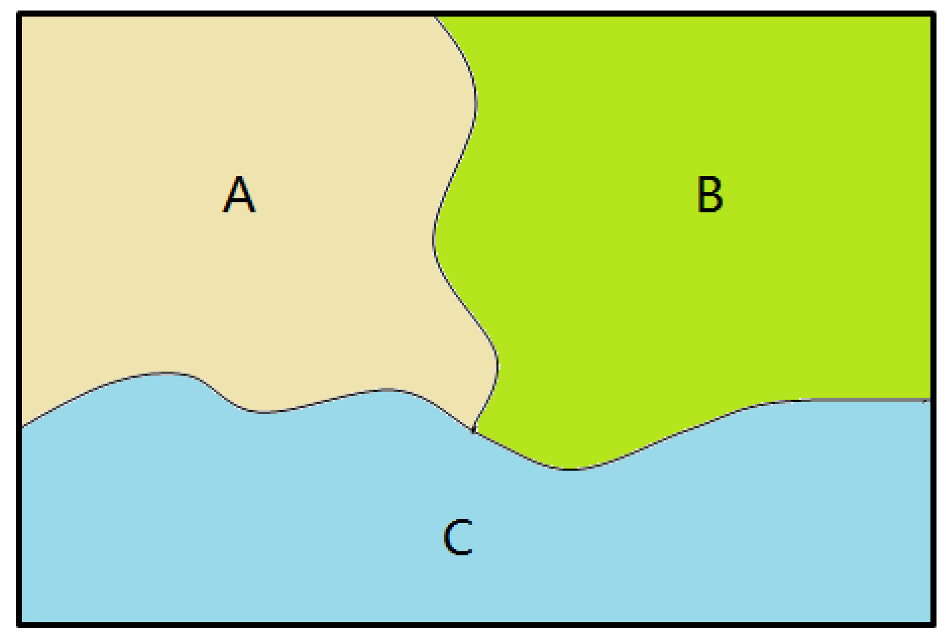
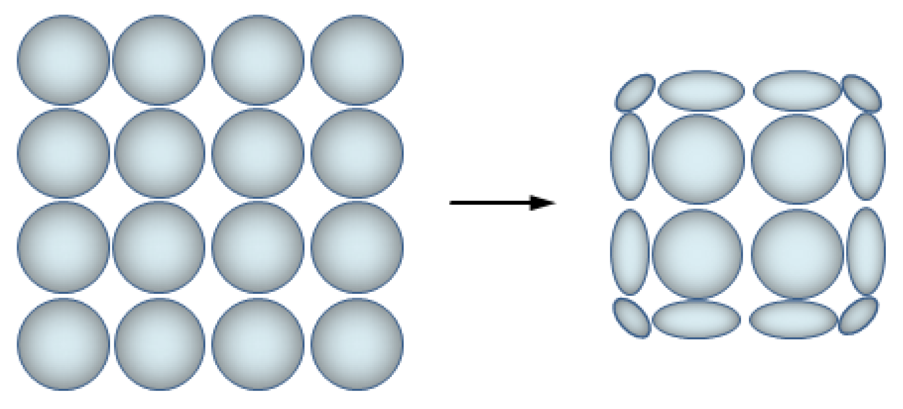
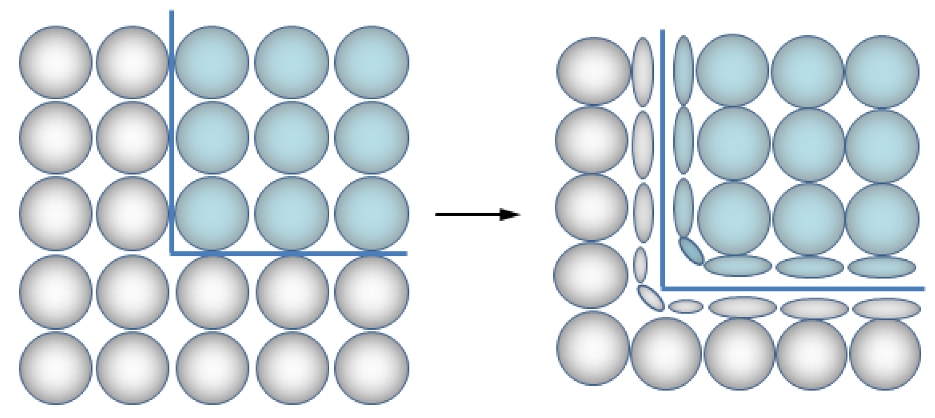
5. Surface Extraction Using Asymmetric Kernels

Traditionally, the color field [5] can be written as:

$$\varphi \left(\mathbf{x}\right)=\sum _j\frac{m_j}{{\rho }_j}W(\mathbf{x}-{\mathbf{x}}_j,h_j).$$

(22)

In this equation, W is the symmetric kernel function, and it can be expressed as:

$$W(\mathbf{r},h)=\frac{\sigma }{h^d}P\left(\frac{\left|\right|\mathbf{r}\left|\right|}{h}\right)$$

(23)

where $\sigma$ is a scaling factor, while $\mathbf{r}$ is a radial vector, d represents the dimension of the simulation space, and P is a finite-supported symmetric decaying spline.

To deal with the badly-distributed density near the surface, the asymmetric kernel approach [1] smooths the location of the kernel center ${\mathbf{x}}_i$ using one step of diffusion to ensure denoising. The refined kernel center ${\overline{\mathbf{x}}}_j$ can be represented as:

$${\overline{\mathbf{x}}}_i=\left(1-\lambda \right){\mathbf{x}}_i+\lambda \sum _j{w}_{ij}{\mathbf{x}}_j/\phantom{\sum _j{w}_{ij}{\mathbf{x}}_j\sum _j{w}_{ij}}\sum _j{w}_{ij}$$

(24)

where $0<\lambda <1$ and w is the weighted function.

The asymmetric kernel method [1] can get the density distribution with more details by using h instead of a $d\times d$ real positive definite matrix G, and it makes W an asymmetric kernel:

$$W(\mathbf{r},\mathbf{G})=\sigma det\left(\mathbf{G}\right)P\left(∥\mathbf{Gr}∥\right)$$

(25)

where $\mathbf{r}=x-{\overline{x}}_j$, the x in it can be regarded as an arbitrary position, and the matrix G is used to rotate and stretch the radial vector r.

After that, the asymmetric kernel approach uses Weighted Principal Component Analysis (WPCA) to compute G. The WPCA starts with calculating the data points’ weighted mean. After that, WPCA builds a weighted covariance matrix C and performs eigendecomposition on it. The principal axes will be provided by the resulting eigenvectors. Finally, it builds an asymmetric matrix G with the output of WPCA to match W.

The expression of the covariance matrix can be written as:

$${\mathbf{C}}_i=\sum _j{w}_{ij}({\mathbf{x}}_j-{\overline{\mathbf{x}}}_i){({\mathbf{x}}_j-{\overline{\mathbf{x}}}_i)}^{\mathrm{T}}/\phantom{\sum _j{w}_{ij}({\mathbf{x}}_j-{\overline{\mathbf{x}}}_i){({\mathbf{x}}_j-{\overline{\mathbf{x}}}_i)}^{\mathrm{T}}\sum _j{w}_{ij}}\sum _j{w}_{ij}$$

(26)

The weighted mean of particle i applied by the asymmetric kernel approach is written as:

$${\overline{\mathbf{x}}}_i=\sum _j{w}_{ij}{\mathbf{x}}_j/\phantom{\sum _j{w}_{ij}{\mathbf{x}}_j\sum _j{w}_{ij}}\sum _j{w}_{ij}$$

(27)

The function $w_{ij}$ is an symmetric weighted function:

$$w_{ij}=\left\{\begin{array}{cc}1-{\left(\frac{∥{\mathbf{x}}_i-{\mathbf{x}}_j∥}{l_i}\right)}^3\hfill & ∥{\mathbf{x}}_i-{\mathbf{x}}_j∥<l_i\hfill \\ 0\hfill & \mathrm{other}\hfill \end{array}\right.$$

(28)

where $l_i$ is the radius of the neighbor scope. To get adequate neighbors and gain sensible asymmetric data, we set $l_i=2h_i$.

For each of the particles, they require Singular Value Decomposition (SVD) on the covariance matrix ${\mathbf{C}}_i$, that is:

$${\mathbf{C}}_i=\mathbf{R}\mathsf{\Sigma }{\mathbf{R}}^{\mathrm{T}}$$

(29)

By using principal axes as column vectors, R is a rotation matrix. $\mathsf{\Sigma }=diag({\sigma }_1,\cdots ,{\sigma }_d)$.

R is a $3\times 3$ rotation matrix using the eigenvectors of ${\mathbf{C}}_i$ as column vectors in the above formulas. In each column, ${\mathbf{R}}_i$ is the distribution axis of ${\mathbf{C}}_i$ corresponding to the eigenvalue ${\sigma }_i$ in $\mathsf{\Sigma }$. $\mathsf{\Sigma }$ is a diagonal matrix with eigenvalues ${\sigma }_1\ge \cdots {\sigma }_d$, so the quantity of neighbor particles is the largest in the direction ${\mathbf{R}}_1$ and the smallest in the ${\mathbf{R}}_3$ axis. In order to avoid extreme conditions and unexpected situations from occurring, the asymmetric kernel method also modifies the matrix ${\mathbf{C}}_i$. First, we modify ${\sigma }_i$, if ${\sigma }_1/{\sigma }_d\ge k_r$, and then, ${\sigma }_i$ is replaced by ${\sigma }_1/k_r$. After that, it uses $\mathbf{G}=k_n\mathbf{I}$ to replace asymmetric kernels for isolated particles and internal fluid particles. The modified ${\mathbf{C}}_i$ can be expressed as:

$${\tilde{\mathbf{C}}}_i=\mathbf{R}\tilde{\mathsf{\Sigma }}{\mathbf{R}}^{\mathrm{T}}$$

(30)

$$\tilde{\mathsf{\Sigma }}=\left\{\begin{array}{c}{k}_{s}diag({\sigma }_1,{\tilde{\sigma }}_1\cdots ,{\tilde{\sigma }}_d)N>N_t\hfill \\ k_n\mathbf{I}\mathrm{other}\hfill \end{array}\right.$$

(31)

where ${\tilde{\sigma }}_i=max({\sigma }_i,{\sigma }_1/k_r)$, N represents the quantity of neighborhoods and $N_t$ indicates the threshold. Asymmetric kernel method assures $∥k_s\mathbf{C}∥\approx 1$ and $k_n=0.5$, $N_t=25$ by employing $k_r=4$, $k_s=1400$.

In order to enable W to transform smoothly in accordance with ${\tilde{\mathbf{C}}}_i$ while maintaining the former form, G should be written as:

$$\mathbf{G}=\frac{1}{h}\mathbf{R}{\tilde{\mathsf{\Sigma }}}^{-1}{\mathbf{R}}^{\mathrm{T}}$$

(32)

6. Asymmetric Surface Extraction for Multiple-Phase Interfaces

6.1. Asymmetric Kernel for Multiple-Phase Interfaces

In principle, the asymmetric surface extraction method is regarded as a level set method. It usually uses various level set functions on each phase to construct the multiphase interface. Therefore, it is also known as the multiple level set method. Next, it constructs surfaces of the fluids on the basis of the various level set functions. However, applying multiple level set methods directly is inclined to evoke errors at the interface. While applying the symmetric approach [5], the overlapping issue arises in the multiphase interface. What is more, a worse overlapping problem or crack issue at the interface will arise when using the asymmetric surface construction algorithm.

Figure 3 exhibits an instance of the symmetrical kernel function becoming an asymmetric function. The balls and the ellipsoids are the scope of the particles’ kernels. The left side of the picture is the symmetrical kernel, while the right side shows the asymmetric kernel. We can see that after asymmetric transition, next to the fluid’s surface, the smooth kernel transforms from round particles to ellipsoid particles, while the internal particles’ smoothing kernel remains original. Therefore, the multiphase interface tends to exhibit an appearance that looks alike while using the asymmetric surface reconstruction approach combined with the multiple level set method, which can be seen in Figure 4. In Figure 4 (left), the symmetrical kernel approach is given, while the right figure is the asymmetric kernel approach. We can obviously see that particles next to the interface have a lack of neighbors. For the sake of including more neighbors at the interface, the asymmetric kernel method will deform the smooth kernel, so that particles’ kernels near the interface are deformed into ellipsoids. Nevertheless, on the basis of a multiple level set, the reconstructed fluid surfaces have obvious voids at the multiphase interface due to a lack of consideration of the influence of other phases’ particles, which would jeopardize the rendering process severely in the following.

To handle the non-uniform distribution of the particles and reduce noises, the asymmetric kernel approach would apply the Laplacian smoothing technique at the center of the kernel (as shown in Equation (9)). This procedure can significantly reduce the irregular condition. For the reason that most of the neighbors of particles next to the surface are inside, the fluid volume is compressed slightly, and the whole fluid shrinks inwardly. It is quite simple to figure out that the smoothing can result in the voids of the multiphase interface, as well.

When building the fluid surface according to phases using the multiple level set approach, overlap appearance would occur at the multiphase interface. This is common when using the level set approach. As shown in Figure 5, the overlap phenomenon occurs at the fluid interface when reconstructing the two-phase surface. The left side of the figure indicates the perfect simulated fluid surface, and the middle of the figure indicates the reconstructed fluid surfaces with the multiple level set, while the right shows the surface in the whole domain. As the color field approach [5] belongs to the level set approach, we study the cause of the overlapping problem of the multiphase interface using the color field approach as an example. As shown in Figure 5, the blue fluid value was 10, and the green fluid value was 20. The value of the blue ones next to the surface reduces from 10–0 linearly, while the green ones’ value next to the surface decreases from 20–0. Now, if a unified color field value is selected to build the surface of the whole fluid domain, overlaps would occur at the two-phase interface. This is due to fact that next to the surface, there are overlapping areas (10–0 or 20–0) for the color field values of the two fluids. Therefore, when selecting a unified color field value to build the whole fluid surface, the two-phase fluid interface will intersect. For instance, to rebuild the whole surface of the fluid domain, we can set the color field to zero, as shown in the right of Figure 5 (however, overlapping problems with other values still remain).

To decrease the surface reconstruction defects during the simulation as much as possible, we took the contribution of other phases into account when tracking the fluid surface from each kind of fluid and handled them with some specific measures.

First of all, because the formula of kernel centers applied by the asymmetric surface reconstruction approach only take the contribution of its own phase into account, Equation (24) is updated as follows:

$${{\overline{\mathbf{x}}}^{\prime }}_i=\left(1-\lambda \right){\mathbf{x}}_i+\lambda \sum _k^n\sum _j{w}_{ikj}{\mathbf{x}}_{kj}/\phantom{\sum _j{w}_{ikj}{\mathbf{x}}_{kj}\sum _j^n\sum _j{w}_{ikj}}\sum _j^n\sum _j{w}_{ikj}$$

(33)

$\lambda$ is a constant between zero and one, and w represents the weight function, while n is the quantity of phases.

Likewise, we modify the covariance matrix from Equation (26) as:

$${{\mathbf{C}}^{\prime }}_i=\sum _k^n\sum _j{w}_{ikj}({\mathbf{x}}_j-{\overline{\mathbf{x}}}_i){({\mathbf{x}}_j-{\overline{\mathbf{x}}}_i)}^{\mathrm{T}}/\phantom{\sum _k^n\sum _j{w}_{ikj}({\mathbf{x}}_j-{\overline{\mathbf{x}}}_i){({\mathbf{x}}_j-{\overline{\mathbf{x}}}_i)}^{\mathrm{T}}\sum _k^n\sum _j{w}_{ikj}}\sum _k^n\sum _j{w}_{ikj}$$

(34)

In this formula, $w_{ikj}$ is the weight function that takes the distance between particles i and j into account. $w_{ikj}$ is written as:

$$w_{ikj}=\left\{\begin{array}{cc}1-{\left(\frac{∥{\mathbf{x}}_i-{\mathbf{x}}_j∥}{l_i}\right)}^3\hfill & ∥{\mathbf{x}}_i-{\mathbf{x}}_j∥<l_i\hfill \\ 0\hfill & \mathrm{other}\hfill \end{array}\right.$$

(35)

where $l_i$ indicates the support radius, k is the phase, which has no influence on the weighted function, and $w_{ikj}$ is just like the one in Equation (28).

On the basis of the covariance matrix in Equation (34), we produce matrix ${\mathbf{G}}^{\prime }$ similar to matrix G as:

$${\mathbf{G}}^{\prime }=\frac{1}{h}{\mathbf{R}}^{\prime }{\widetilde{{\mathsf{\Sigma }}^{{}^{\prime }}}}^{-1}{{\mathbf{R}}^{\prime }}^{\mathrm{T}}$$

(36)

Overall, the color field that is used to extract surface from all phases is written as:

$${\varphi }^{\prime }\left(\mathbf{x}\right)=\sum _j\frac{m_j}{{\rho }_j}W(\mathbf{x}-{\mathbf{x}}_j,{{\mathbf{G}}^{\prime }}_j)$$

(37)

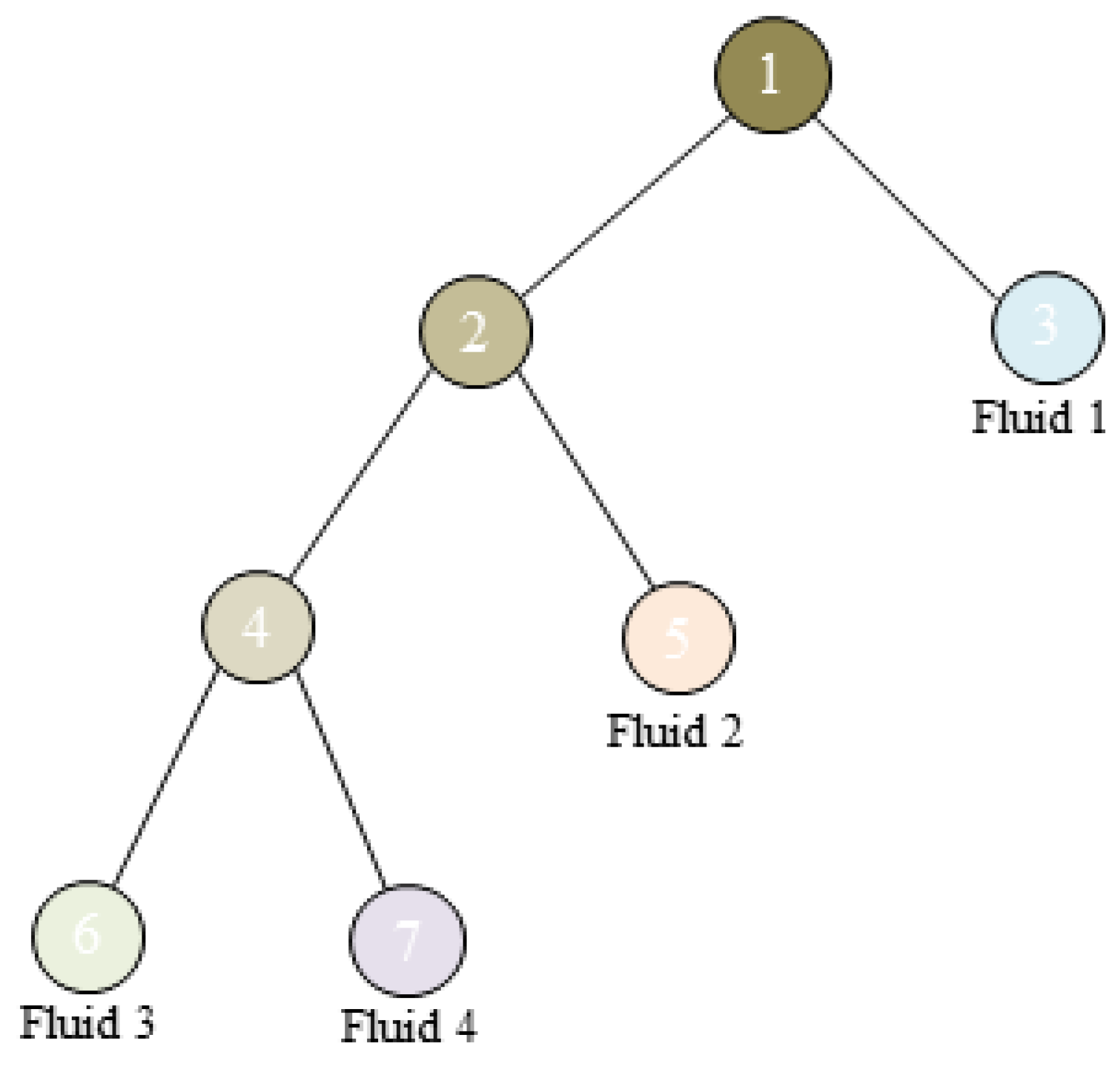
6.2. Surface Extraction Strategy

In the instance of Figure 5, we used the color field as an Unsigned Distance Field (USDF). The USDF is typically good at surface reconstruction, and we devised the Signed Color Field (SDF) for a better extraction of the multiphase interface with the strategy we employed as the “binary tree” used to extract the surface, as shown in Figure 6.

We demonstrated our reconstruction scheme with a four-phase fluid simulation, as shown in Figure 6. In this figure, Nodes 1, 2, and 4 indicate the fluid interface of the four-phase, three-phase, and two-phase, respectively, and Nodes 3, 5, 6, and 7 represent four different kinds of fluids, respectively. When reconstructing the fluid surface, we only extracted one phase from the entire fluid domain at a time in the iteration. This is because we were able to apply the symmetrical color field with positive and negative values (signed color field) to distinguish the two-phase interface when expressing the fluid surface. The signed color field could make the color field values between two-phase interface transit uniformly from negative to positive. When we want to extract the surface of Fluid 1 (Node 3) and the surface of the other phases (Node 2) from the four-phase fluid (Node 1), we employ the color field for ${\varphi }^{\prime }\left(x\right)=1$ and ${\varphi }^{\prime \prime }\left(x\right)=-{\varphi }^{\prime }\left(x\right)$, respectively. According to this method, two kinds of fields can be interpolated using Equation (37), where one represents the fluid domain of Fluid 1 and the other denotes the fluid domain of the other three phases. Then, we can reconstruct fluid surfaces of Fluid 1 and the other three phases based on the interpolated two kinds of field values. In terms of choosing the field values for surface reconstruction, we used $\epsilon {\varphi }^{\prime }\left(x\right)$, $-\epsilon {\varphi }^{\prime }\left(x\right)$ ($0<\epsilon <0.1$, and we set $\epsilon =0.01$) to construct the surface. In this way, we can ensure that the reconstructed fluid surface is approximately one face at the multiphase interface without serious vacuums and overlaps. Then, we extracted the surface of Fluid 2 and the other two phases from the remaining three phases in the same manner. By repeating the step mentioned above, we can eventually reconstruct the surface of Fluids 3 and 4. In conclusion, the fluid surface can be separately extracted for each phase using our “binary tree” scheme, which preserve voids and overlaps between interfaces.

In other words, the multiphase fluid (n-phase) surface reconstruction strategy we proposed can be summarized as follows:

• Initially, employ two color fields ${\varphi }^{\prime }\left(x\right)$ and $-{\varphi }^{\prime }\left(x\right)$ for the particles for one phase and then the rest of the $n-1$ phases, respectively;
• Additionally, interpolate the signed color field for one phase and the other n-1 phases, and then, select $\epsilon {\varphi }^{\prime }\left(x\right)$, $-\epsilon {\varphi }^{\prime }\left(x\right)$ separately as the surface field value;
• Furthermore, on the basis of the chosen surface field value, rebuild the surface for the one phase;
• Finally, iterate the procedures above until the surface of each phase is fully rebuilt.

There are several advantages of our surface reconstruction scheme for the multiphase interface. One thing is that the color field approach forces the values to be reduced linearly from $\varphi \left(x\right)$ to zero next to the fluid surface approximately. Applying the signed color field enables values to be decreased linearly from positive to zero, and gradually decreased to negative at the two-phase interface. Therefore, it enables the surface to be reconstructed uniformly at two-phase interface. Overall, we can avoid the averagely-divided biases of the interface area, or it might have voids or overlaps. The other issue is that selecting a relatively small value for the surface field $\epsilon {\varphi }^{\prime }\left(x\right)$, $-\epsilon {\varphi }^{\prime }\left(x\right)$ guarantees that no further area would be rebuilt. It is simple to prevent reconstructing the domain that does not belong to the fluid surface when the values of the color field look pretty much the same as the fluid surface. Furthermore, since $\epsilon {\varphi }^{\prime }\left(x\right)$ is small enough, we can assumably regard the multiphase interface as one interface without overlaps.

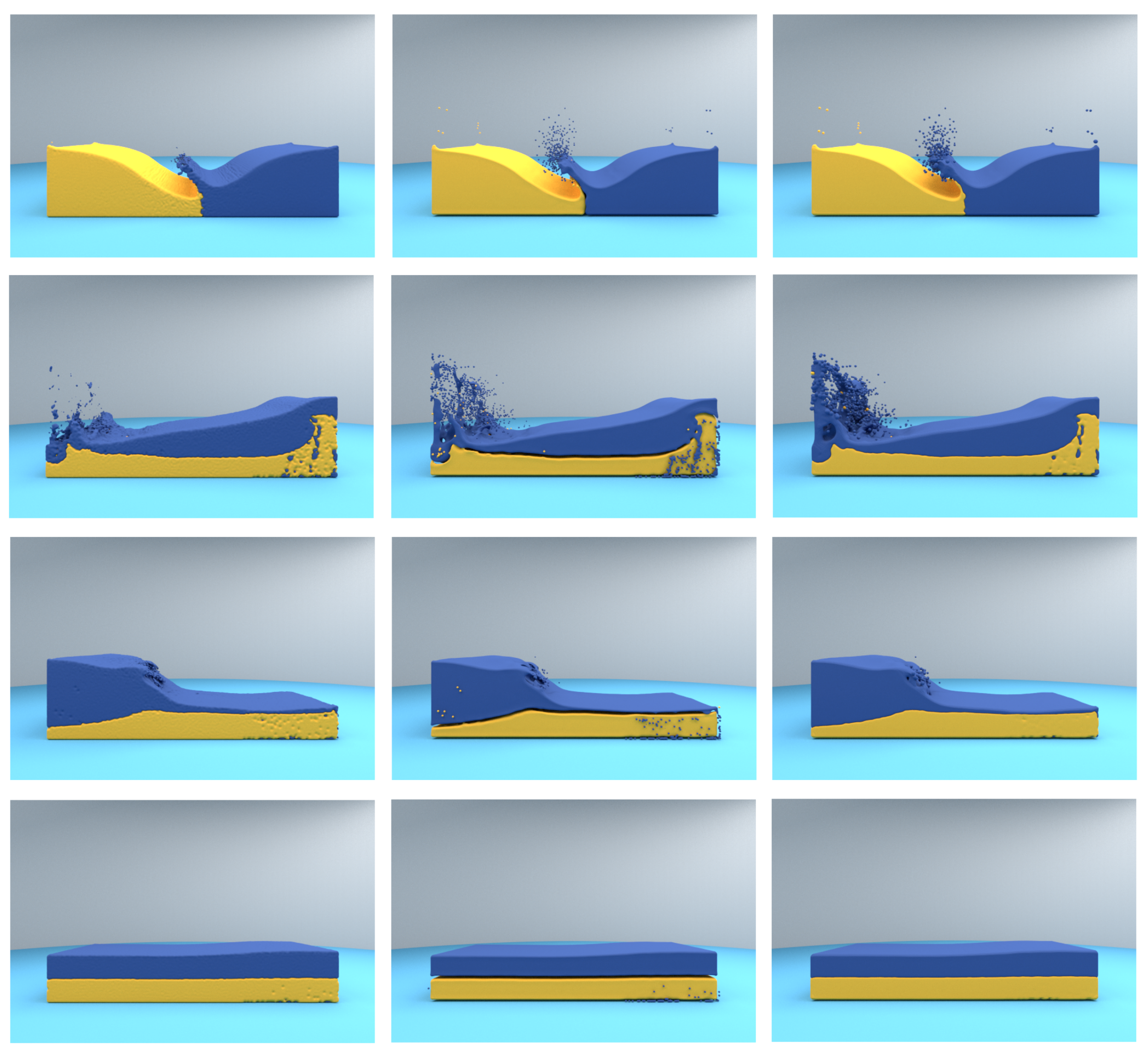
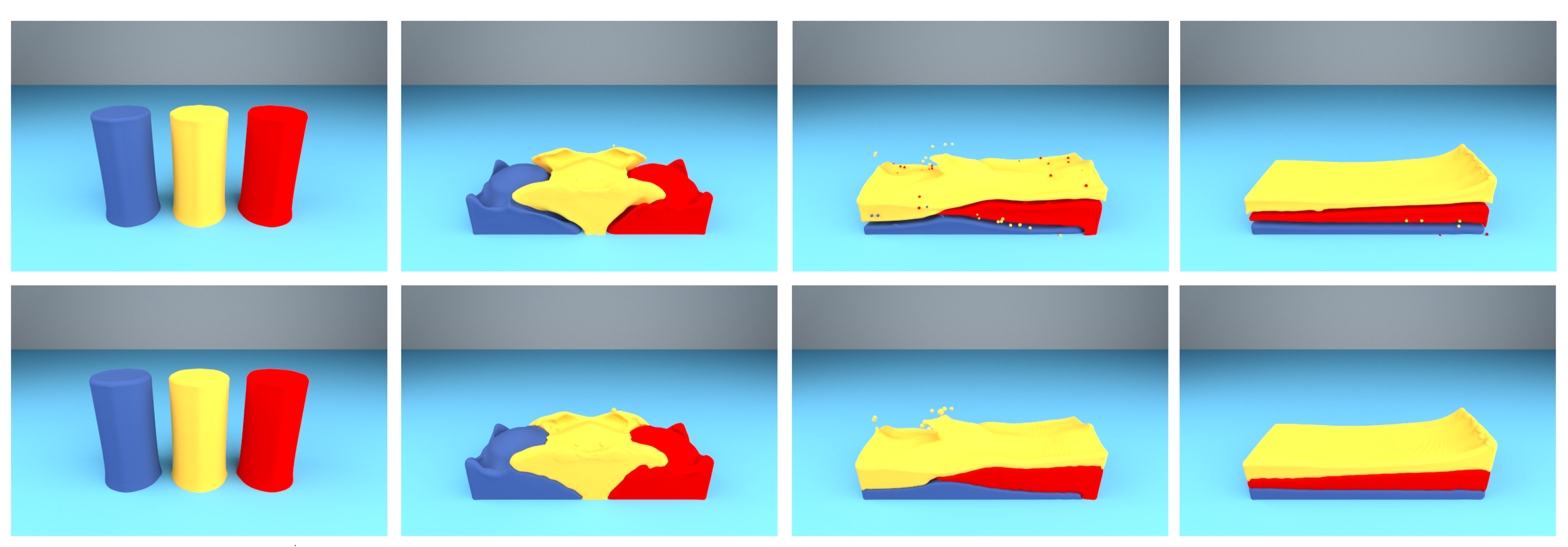
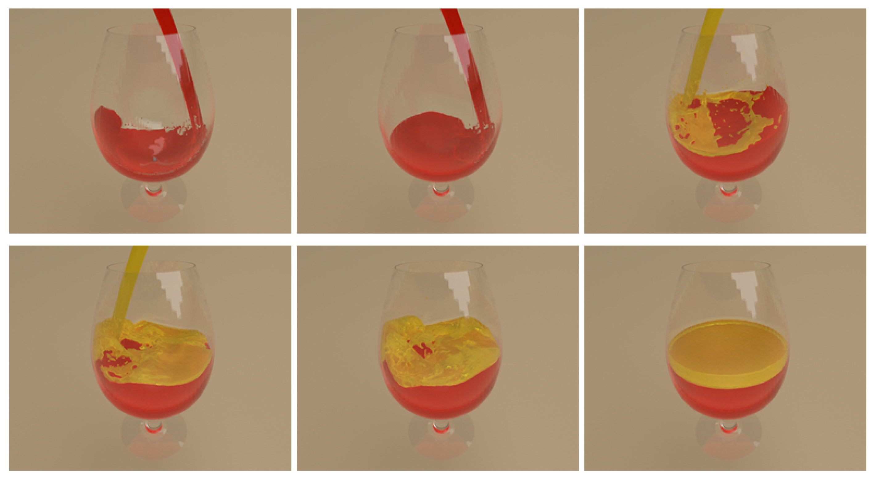
7. Implementation and Results

We carried out a few experiments to exhibit the credibility of multiphase fluid simulation, as mentioned above. The experiments were achieved with C++. Meanwhile, OpenMP was used for parallelization. The neighbor search process was achieved with the spatial Hash method with a width uniform space background mesh. We used the marching cubes algorithm as the surface reconstruction method for the multiphase interface presented in this paper to extract the fluid surfaces. With the help of the Open Graphics Library (OpenGL) (The Khronos Group, Beaverton, OR, USA), a real-time simulation was presented, and offline high quality rendering was carried out with Blender’s ray tracing engine cycles. The experiments were carried out on a graphic workstation with an Intel Xeon E5-2637 v2 (15M Cache, 3.50 GHz @ 4 cores) CPU, 80 gigabytes RAM, NVIDIA Quadro K4000 GPU (Dell, Round Rock, TX, USA).

Figure 7 shows the simulation outcomes of the symmetric kernel approach [5], the asymmetric kernel approach [1], and our approach in a breaking dam simulation with two phases. The key parameters of this scene can be seen in

Table 1. The parameters of the two-phase breaking dam simulation.

Parameter	Value
Size of domain	24 m × 24 m × 24 m
Smoothing kernel	Cubic splines
Number of blue particles	126 k
Number of yellow particles	126 k
Density of blue phase	200 $\mathrm{kg}/\phantom{\mathrm{kg}{\mathrm{m}}^3}{\mathrm{m}}^3$
Density of yellow phase	1000 $\mathrm{kg}/\phantom{\mathrm{kg}{\mathrm{m}}^3}{\mathrm{m}}^3$
Support radius	0.2 m
Diameter of fluid particle	0.1 m

. The setting of the two-phase breaking dam can be described as two cuboids consisting of different fluid phases affected by gravity falling from the start, after two-phase fluids come in contact and gradually blending. Then, with the influence of pressure and interface force, the fluid with a lesser density will “float” gradually, while the other fluid with a greater density would start to “sink”. The shape of the fluids is gradually stabilized, and they are split into two layers with a distinct interface. In Figure 7a, it is clear that the multiphase fluid surface rebuilt using the symmetric kernel approach was crude overall. What is worse, there were overlaps and voids at the two-phase interfaces. Further, the surface appearance was weak after rendering. Figure 7b illustrates the fluid surface rebuilt through the asymmetric kernel approach, which was smoother than the symmetric kernel method. However, at the two-phase interface, there were noticeable voids, which contaminated the simulation fidelity badly. In Figure 7c, one can find that the fluid surface rebuilt using our approach was relatively smoother with no voids or overlaps at the two-phase interfaces. The ideal appearance proved that our approach can simulate two-phase fluids’ interaction effectively and accurately.

Figure 8 shows the results of the asymmetric kernel approach [1] and our approach in the breaking dam simulation in a cylinder of fluid with three phases. The key parameters and statistics of this scene can be seen in

Table 2. The parameters of two-phase breaking dam simulation.

Parameter	Value
Size of domain	24 m × 24 m × m
Smoothing kernel	Cubic splines
Number of blue particles	13,325
Number of yellow particles	13,325
Number of red particles	13,325
Density of red phase	300 $\mathrm{kg}/\phantom{\mathrm{kg}{\mathrm{m}}^3}{\mathrm{m}}^3$
Density of blue phase	900 $\mathrm{kg}/\phantom{\mathrm{kg}{\mathrm{m}}^3}{\mathrm{m}}^3$
Density of yellow phase	100 $\mathrm{kg}/\phantom{\mathrm{kg}{\mathrm{m}}^3}{\mathrm{m}}^3$
Support radius	0.2 m
Diameter of fluid particle	0.1 m

. The procedure of this experiment was as follows. First, with the influence of the gravity, all phases were falling and contacting and gradually started to blend. Second, the fluid with a lesser density floated as the simulation continued, while the fluid with a greater density gradually sunk. Since the density of the yellow fluid was the least, it flowed right to the top. Third, the three-phase fluids collided with each other and were fully mixed. Finally, the movement of the fluids was gradually stabilized, and fluids were split into three layers with two fine interfaces. Figure 8a shows the asymmetric kernel approach. At three-phase interfaces, there still remained distinct voids, which resulted in poor appearance. Figure 8b further demonstrates the effectiveness of our method. The results of our approach in the three-phase flow simulation showed a smooth and flat surface appearance, which had no voids or overlaps.

Figure 9 shows a two-phase cocktail scenario using our surface reconstruction method. There were 30,005 particles of yellow fluid and 109,802 particles of red fluid. The density of the yellow fluid was 300 $\mathrm{kg}/\phantom{\mathrm{kg}{\mathrm{kg}}^3}{\mathrm{kg}}^3$ and the density of the red fluid was 1000 $\mathrm{kg}/\phantom{\mathrm{kg}{\mathrm{kg}}^3}{\mathrm{kg}}^3$. In this experiment, one phase fluid was poured into a goblet, then another fluid phase began to be injected. From this scene, it is proven that our method was able to simulate the multiphase fluid with better surface and interface effects.

8. Conclusions

We introduced an easy, yet quite effective multiphase fluid simulation approach using asymmetric surface extraction and a modified density model. The novel surface extraction scheme considered the issue of overlaps and gaps, which rebuilt the multiphase fluid surface with a multiple level set and asymmetric kernel. What is more, the “binary tree” strategy and adapted asymmetric kernel were employed to extract surfaces. In addition, we integrated it with a multiphase fluid model derived by the number density to eliminate density deviations at interfaces. The results showed that our approach can erase the voids and overlaps at the multiphase interface and can simulate the interaction of multiphase fluid accurately. In brief, our approach was capable of particle-based simulation and 3D visualization of a multiphase fluid. Our proposed method could be extended to a large-scale scene and multiphase diffusion and convection simulation in future work.

References

1. Yu, J.; Turk, G. Reconstructing surfaces of particle-based fluids using anisotropic kernels. ACM Trans. Graphics 2013, 32. [Google Scholar] [CrossRef]
2. Wang, X.; Ban, X.; Zhang, Y.; Pan, Z.; Liu, S. Anisotropic Surface Reconstruction for Multiphase Fluids. In Proceedings of the 2017 International Conference on Cyberworlds, Chester, UK, 20–22 September 2017; pp. 118–125. [Google Scholar]
3. Boulic, R.; Hégron, G. Smoothed particles: A new paradigm for animating highly deformable bodies. In Computer Animation and Simulation; Boulic, R.; Hégron, G. Spring: Vienna, Austria, 1994; pp. 61–76. [Google Scholar]
4. Monaghan, J.J. Simulating free surface flows with SPH. J. Comput. Phys. 1996, 110, 399–406. [Google Scholar] [CrossRef]
5. Muller, M.; Charypar, D.; Gross, M. Particle-based fluid simulation for interactive applications. In Proceedings of the 2003 ACM SIGGRAPH/Eurographics Symposium on Computer Animation, San Diego, CA, USA, 26–27 July 2003; pp. 154–159. [Google Scholar]
6. Becker, M.; Teschner, M. Weakly compressible SPH for free surface flows. In Proceedings of the 2007 ACM SIGGRAPH/Eurographics Symposium on Computer Animation, San Diego, CA, USA, 2–4 August 2007; pp. 209–217. [Google Scholar]
7. Solenthaler, B.; Pajarola, R. Predictive-corrective incompressible SPH. ACM Trans. Graphics 2009, 28, 40. [Google Scholar] [CrossRef]
8. He, X.; Liu, N.; Li, S.; Wang, H.; Wang, P. Local Poisson SPH For Viscous Incompressible Fluids. Comput. Graphics Forum 2012, 31, 1948–1958. [Google Scholar] [CrossRef]
9. Ihmsen, M.; Cornelis, J.; Solenthaler, B.; Horvath, C.; Teschner, M. Implicit Incompressible SPH. IEEE Trans. Visual Comput. Graphics 2014, 20, 426–435. [Google Scholar] [CrossRef] [PubMed]
10. Bender, J.; Koschier, D. Divergence-free smoothed particle hydrodynamics. In Proceedings of the 2015 ACM SIGGRAPH / Eurographics Symposium on Computer Animation, Los Angeles, CA, USA, 7–9 August 2015; pp. 147–155. [Google Scholar]
11. Hoover, W.G. Isomorphism linking smooth particles and embedded atoms. Physica A 1998, 260, 244–254. [Google Scholar] [CrossRef]
12. Agertz, O.; Moore, B.; Stadel, J.; Potter, D.; Miniati, F.; Read, J.; Mayer, L.; Gawryszczak, A.; Kravtsov, A. Fundamental differences between SPH and grid methods. Mon. Not. of the R. Astron. Soc. 2007, 380, 963–978. [Google Scholar] [CrossRef] [Green Version]
13. Ott, F.; Schnetter, E. A modified SPH approach for fluids with large density differences. arXiv 2003, arXiv:physics/0303112. [Google Scholar]
14. Tartakovsky, A.M.; Meakin, P. A smoothed particle hydrodynamics model for miscible flow in three-dimensional fractures and the two-dimensional Rayleigh–Taylor instability. J. Comput. Phys. 2005, 207, 610–624. [Google Scholar] [CrossRef]
15. Hu, X.Y.; Adams, N.A. A multi-phase SPH method for macroscopic and mesoscopic flows. J. Comput. Phys. 2006, 213, 844–861. [Google Scholar] [CrossRef]
16. Kang, M.; Fedkiw, R.P.; Liu, X.D. A boundary condition capturing method for multiphase incompressible flow. J. Sci. Comput. 2000, 15, 323–360. [Google Scholar] [CrossRef]
17. Pelupessy, F.I.; Schaap, W.E.; Van De Weygaert, R. Density estimators in particle hydrodynamics-DTFE versus regular SPH. Astron. Astrophys. 2003, 403, 389–398. [Google Scholar] [CrossRef]
18. Hong, J.M.; Kim, C.H. Discontinuous fluids. ACM Trans. Graphics 2005, 24, 915–920. [Google Scholar] [CrossRef]
19. Hong, J.M.; Kim, C.H. Animation of bubbles in liquid. Comput. Graphics Forum 2003, 22, 253–262. [Google Scholar] [CrossRef]
20. Mihalef, V.; Unlusu, B.; Metaxas, D.; Sussman, M.; Hussaini, M.Y. Physics based boiling simulation. In Proceedings of the 2006 ACM SIGGRAPH/Eurographics symposium on Computer animation, Vienna, Austria, 2–4 September 2006; pp. 317–324. [Google Scholar]
21. Zheng, W.; Yong, J.H.; Paul, J.C. Simulation of bubbles. In Proceedings of the ACM SIGGRAPH/Eurographics symposium on Computer animation, Vienna, Austria, 2–4 September 2006; pp. 325–333. [Google Scholar]
22. Losasso, F.; Talton, J.O.; Kwatra, N.; Fedkiw, R. Two-way coupled SPH and particle level set fluid simulation. IEEE Trans. Visual Comput. Graphics 2008, 14, 797–804. [Google Scholar] [CrossRef] [PubMed]
23. Thürey, N.; Sadlo, F.; Schirm, S.; Muller-Fishcer, M.; Gross, M. Real-time simulations of bubbles and foam within a shallow water framework. In Proceedings of the 2007 ACM SIGGRAPH/Eurographics Symposium on Computer Animation, San Diego, CA, USA, 2–4 August 2007; pp. 191–198. [Google Scholar]
24. Müller, M.; Solenthaler, B.; Keiser, R.; Gross, M. Particle-based fluid-fluid interaction. In Proceedings of the 2005 ACM SIGGRAPH/Eurographics Symposium on Computer Animation, Los Angeles, CA, USA, 29–31 July 2005; pp. 237–244. [Google Scholar]
25. Mao, H.; Yang, Y.H. Particle-based immiscible fluid-fluid collision. In Proceedings of the Graphics Interface 2006, Quebec, QC, Canada, 7–9 June 2006; pp. 49–55. [Google Scholar]
26. Solenthaler, B.; Pajarola, R. Density contrast SPH interfaces. In Proceedings of the 2008 ACM SIGGRAPH/Eurographics Symposium on Computer Animation, Dublin, Ireland, 7–9 July 2008; pp. 211–218. [Google Scholar]
27. Blinn, J.F. A generalization of algebraic surface drawing. ACM Trans. Graphics 1982, 1, 235–256. [Google Scholar] [CrossRef]
28. Zhu, Y.; Bridson, R. Animating sand as a fluid. ACM Trans. Graphics 2005, 24, 965–972. [Google Scholar] [CrossRef]
29. Adams, B.; Pauly, M.; Keiser, R.; Guibas, L.J. Adaptively sampled particle fluids. ACM Trans. Graphics 2007, 26, 48. [Google Scholar] [CrossRef]
30. Bhatacharya, H.; Gao, Y.; Bargteil, A. A level-set method for skinning animated particle data. In Proceedings of the 2011 ACM SIGGRAPH/Eurographics Symposium on Computer Animation, Vancouver, BC, Canada, 5–7 August 2011; pp. 17–24. [Google Scholar]
31. Yu, J.; Wojtan, C.; Turk, G.; Yap, C. Explicit mesh surfaces for particle based fluids. Comput. Graphics Forum 2012, 31, 815–824. [Google Scholar] [CrossRef]
32. Akinci, G.; Ihmsen, M.; Akinci, N.; Teschner, M. Parallel surface reconstruction for particle-based Fluids. Comput. Graphics Forum 2012, 31, 1797–1809. [Google Scholar] [CrossRef]
33. Akinci, G.; Akinci, N.; Ihmsen, M.; Matthias, T. An efficient surface reconstruction pipeline for particle-based fluids. In Workshop on Virtual Reality Interaction and Physical Simulation; Bender, J., Kuijper, A., Fellner, D.W., Guerin, E., Eds.; The Eurographics Association: Zürich, Switzerland, 2012; pp. 61–68. [Google Scholar]
34. Osher, S.; Fedkiw, R. Level Set Methods and Dynamic Implicit Surfaces. Springer: New York, NY, USA, 2002. [Google Scholar]
35. Losasso, F.; Shinar, T.; Selle, A.; Fedkiw, R. Multiple interacting liquids. ACM Trans. Graphics 2006, 25, 812–819. [Google Scholar] [CrossRef]
36. Kim, B. Multi-phase fluid simulations using regional level sets. ACM Trans. Graphics 2010, 29, 175. [Google Scholar] [CrossRef]
37. Saye, R.I.; Sethian, J.A. Analysis and applications of the Voronoi implicit interface method. J. Comput. Phys. 2012, 231, 6051–6085. [Google Scholar] [CrossRef]
38. Starinshak, D.P.; Karni, S.; Roe, P.L. A new level set model for multimaterial flows. J. Comput. Phys. 2014, 262, 1–16. [Google Scholar] [CrossRef]
39. Da, F.; Batty, C.; Grinspun, E. Multimaterial mesh-based surface tracking. ACM Trans. Graphics 2014, 33, 1–11. [Google Scholar] [CrossRef] [Green Version]
40. Hirt, C.W.; Nichols, B.D. Volume of fluid (VOF) method for the dynamics of free boundaries. J. Comput. Phys. 1981, 39, 201–225. [Google Scholar] [CrossRef]
41. Dyadechko, V.; Shashkov, M. Reconstruction of multi-material interfaces from moment data. J. Comput. Phys. 2008, 227, 5361–5384. [Google Scholar] [CrossRef]
42. Anderson, J.C.; Garth, C.; Duchaineau, M.A.; Joy, K.I. Smooth, volume-accurate material interface reconstruction. IEEE Trans. Visual Comput. Graphics 2010, 16, 802–814. [Google Scholar] [CrossRef] [PubMed]
43. Quan, S.; Schmidt, D.P. A moving mesh interface tracking method for 3D incompressible two-phase flows. J. Comput. Phys. 2007, 221, 761–780. [Google Scholar] [CrossRef]
44. Pons, J.P.; Boissonnat, J.D. A Lagrangian approach to dynamic interfaces through kinetic triangulation of the ambient space. Comput. Graphics Forum 2007, 26, 227–239. [Google Scholar] [CrossRef]
45. Pons, J.P.; Boissonnat, J.D. Delaunay deformable models: Topology-adaptive meshes based on the restricted delaunay triangulation. In Proceedings of the IEEE Conference on Computer Vision and Pattern Recognition, Minneapolis, MN, USA, 17–22 June 2007. [Google Scholar]
46. Quan, S.; Lou, J.; Schmidt, D.P. Modeling merging and breakup in the moving mesh interface tracking method for multiphase flow simulations. J. Comput. Phys. 2009, 228, 2660–2675. [Google Scholar] [CrossRef]
47. Misztal, M.K.; Erleben, K.; Bargteil, A.; Fursund, J.; Christensen, B.B.; Baerentzen, J.A.; Bridson, R. Multiphase flow of immiscible fluids on unstructured moving meshes. IEEE Trans. Visual Comput. Graphics 2014, 20, 4–16. [Google Scholar] [CrossRef] [PubMed]
48. Wicke, M.; Ritchie, D.; Klingner, B.M.; Burke, S.; Shewchuk, J.R.; O’brien, J.F. Dynamic local remeshing for elastoplastic simulation. ACM Trans. Graphics 2010, 29, 49. [Google Scholar] [CrossRef]
49. Clausen, P.; Wicke, M.; Shewchuk, J.R.; O’brien, J.F. Simulating liquids and solid-liquid interactions with lagrangian meshes. ACM Trans. Graphics 2013, 32, 17. [Google Scholar] [CrossRef]
50. Batchelor, G. An Introduction to Fluid Dynamics; Cambridge University Press: Cambridge, UK, 1967. [Google Scholar]
Figure 1. The interaction of three immiscible fluids.
Symmetry 11 00745 g001
Figure 2. Density comparison.
Symmetry 11 00745 g002
Figure 3. The symmetric kernel transformed to the asymmetric kernel.
Symmetry 11 00745 g003
Figure 4. The symmetric kernel transformed to the asymmetric kernel for the multiple-phase interface.
Symmetry 11 00745 g004
Figure 5. The overlapping of the two-phase interface.
Symmetry 11 00745 g005
Figure 6. Surface reconstruction scheme for the multiphase interface.
Symmetry 11 00745 g006
Figure 7. Breaking dam experiment with two phases. (a) left column, symmetric kernel method; (b) middle column, asymmetric kernel method; (c) right column, our own method.
Symmetry 11 00745 g007
Figure 8. Breaking dam experiment with three phases. (a) first row, asymmetric kernel method; (b) second row, our method.
Symmetry 11 00745 g008
Figure 9. Two-phase cocktail.
Symmetry 11 00745 g009