Article

Multi-Criteria Fuzzy-Stochastic Diffusion Model of Groundwater Control System Selection

Faculty of Mining and Geology, University of Belgrade, Belgrade 11000, Serbia
*
Author to whom correspondence should be addressed.
Symmetry 2019, 11(5), 705; https://doi.org/10.3390/sym11050705
Submission received: 28 March 2019 / Revised: 9 May 2019 / Accepted: 14 May 2019 / Published: 23 May 2019
(This article belongs to the Special Issue Multi-Criteria Decision Aid methods in fuzzy decision problems)

Abstract

:
When considering data and parameters in hydrogeology, there are often questions of uncertainty, vagueness, and imprecision in terms of the quantity of spatial distribution. To overcome such problems, certain data may be subjectively expressed in the form of expert judgment, whereby a heuristic approach and the use of fuzzy logic are required. In this way, decision-making criteria relating to an optimal groundwater control system do not always have a numerical value. Groundwater control scenarios (alternatives) are identified through hydrodynamic modeling of the aquifer, providing an indication of their effectiveness. The paper develops a fuzzy-stochastic multi-criteria decision-making model to deal with a topical problem: selection of the most suitable groundwater control system for an open-cast mine. Both real numerical and linguistic variables are used to express the values of all criteria that affect the final decision. In particular, it should be pointed out that the values of the criteria are varied over a predefined time horizon. For mathematical calculations, fuzzy dynamic TOPSIS and the stochastic diffusion process—geometric Brownian motion—were used. The proposed method is tested in a case study: the selection of an optimal groundwater control system for an open-cast mine.

1. Introduction

This paper presents the development of a decision-making model for solving a highly complex and topical problem, such as the selection of a suitable groundwater control system for an open-cast mine. The main function of groundwater control systems is to decrease the groundwater level in order to provide favorable conditions for efficient open-cast mining.
Using the results of previous hydrodynamic analyses, Polomčić & Bajić [1] discuss the design of groundwater control systems and groundwater management scenarios (alternatives) for the Buvač open-cast mine (Bosnia and Herzegovina) through to the projected cessation of mining (2024). In the present paper, multi-criteria decision analysis is applied to select the optimal groundwater management system under complex hydrogeological conditions, in a multiple criteria situation.
Multi-criteria decision analysis (MCDA) is a method that originates from the decision-making theory. It is applied to problems that involve a finite number of decision options, which experts evaluate and rank using the weights of a finite set of evaluation criteria [2]. The method is composed of a series of techniques whose objective is to rank alternatives in the descending order of preference.
The best way scientists can express their opinions is, in fact, everyday verbal communication. It is also a significant source of uncertainty, because the transfer of both information and knowledge is coupled with various ambiguities and imprecisions. This is the reason why fuzzy logic is applied in MCDA, given that its essence is to handle knowledge that can be highly imprecise and expressed verbally. A system is described using expert knowledge instead of differential equations. Knowledge is conveyed in a natural way, by linguistic variables. An overview of case studies from various scientific areas is presented in [3,4].
Many researchers in hydrogeology, and in particular the hydrogeology of the mineral deposits industry, have applied different mathematical approaches to make optimal decisions. Zarghami & Szidarovszky [5] used a fuzzy multi-criteria decision model and stochastic simulation for a water resources management problem in a real case study. Srđević & Medeiros applied [6] the analytic hierarchy process (AHP) to assess water management plans. Ghorbanzadeh et al. [7] used AHP to optimize subsidence susceptibility mapping. Zhang et al. [8] applied the AHP method, integrated interval two-stage stochastic programming (ITSP), and interval linear multi-objective programming (IMOP) for water resources management policies in arid regions with inherent uncertainty. In the case of optimal groundwater control systems, the decision-making criteria need not always be numerical values. Where fuzzy logic is applied to multi-criteria decision-making, the criteria can be described by linguistic variables represented through fuzzy membership and the system can be described by expert judgment [9]. Bajić et al. [9] applied the fuzzy analytic hierarchy process (FAHP) and VIKOR (Eng. multi-criteria optimization and compromise solution) method for selecting the optimal groundwater control system under complex geological and hydrogeological conditions. Also, Sun et al. [10] presented an interesting example of multidisciplinary design optimization of a tunnel boring machine, under complex geological conditions. Golestanifar & Ahangari [11] applied fuzzy extent analysis to select an optimal groundwater lowering technique for mines. The FAHP method is also used to make decisions on groundwater in environmental impact assessment and hydro-environmental management of groundwater resources [12,13,14], and the evaluation of groundwater potential and water inrush risk [15,16]. For flood risk management, Levy [17] applied MCDA and the analytic network process (ANP). The same methodology is used for land settlement susceptibility mapping [18,19]. Roozbahani et al. [20] applied the PROMETHEE method (Preference Ranking Organization Method for Enrichment Evaluations) for decision-making problems in urban water supply management. The fuzzy TOPSIS method (Technique for Order Preference by Similarity of Ideal Solution) is also widely used in hydrogeology. Afshar et al. [21] applied the fuzzy TOPSIS method to select the best trade-offs of critical issues in water resources management. Onu et al. [22] applied the fuzzy TOPSIS method to rank sustainable water supply alternatives. Senent-Aparicio et al. [23] used this method to rank a combination of climate models, in assessing the impact of climate change on headwaters.
Multi-criteria decision making is used for decision making analysis with dynamically changing input data and criteria weight variation during a temporal decision process. The dynamic multiple-criteria decision making methodology is applied in many different scientific fields, such as: air traffic [24], automotive industry [25], construction industry [26], optimization theory in neural science, psychology and system science [27], economics and marketing management [28,29], emergency management [30], and risk analysis [31]. In the present paper, the fuzzy dynamic TOPSIS method is proposed and tested in making an optimal decision about a groundwater control system. Four criteria in which time is a factor are analyzed. Therefore, this is a dynamic multiple-criteria decision-making problem, in which the ranking of the proposed alternatives changes over a defined time horizon. The model was developed on the basis of ranking of proposed alternatives changing over a predefined timeframe and it considers the variability of input parameters.

2. Methodology

This chapter presents the methodology used to develop the decision-making model. Also, the fuzzy dynamic TOPSIS method is summarized. A fuzzy multi-criteria decision-making problem is usually represented in the following matrix form:
D ˜ = [ x ˜ i j ] m × n = [ A / C C 1 C 2 C n A 1 x ˜ 11 x ˜ 12 x ˜ 1 n A 2 A m x ˜ 21 x ˜ m 1 x ˜ 22 x ˜ 2 n x ˜ m 2 x ˜ m n ]
where A = { A 1 , A 2 , , A i } , i = 1 , 2 , , m is the set of alternatives and C = { C 1 , C 2 , , C j } , j = 1 , 2 , , n is the set of criteria. Here x ˜ i j is the fuzzy triangular number that represents the score of the i-th alternative relative to the j-th criterion.
In the multi-criteria decision-making process, sets of scores obtained on different scales are compared (i.e., each criterion has its own dimension). To make the comparison process much easier, it is necessary to create dimensionless space of decision making. For that purpose, the following normalization of the decision-making matrix is applied:
r ˜ i j = x ˜ i j i = 1 m x ˜ i j = ( a i j , b i j , c i j ) i = 1 m ( a i j , b i j , c i j )   j = 1 , 2 , , n
and a normalized decision-making matrix, R ˜ = [ r ˜ i j ] m × n , is obtained.
The multi-criteria decision-making process is significantly influenced by the weights of the criteria. The significant weight of each criterion can be estimated by subjective and objective methods. Subjective methods rely on the expert knowledge of the decision maker, whereas objective methods use mathematical models. Shannon’s entropy approach belongs to the group of objective methods and it will be used here to arrive at the weight of each criterion. The entropy concept measures the uncertainty of the input data in terms of probability [32,33]. The entropy measure of each criterion is computed as follows:
e ˜ j = k i = 1 m r ˜ i j · l n ( r ˜ i j )
where k = ( l n ( m ) ) 1 is the constant which guarantees that 0 e ˜ j 1 . The divergence that indicates the importance of the j-th criterion is:
d ˜ j = 1 e ˜ j
The objective weight of the criterion, based on the entropy concept, is as follows:
w ˜ j = d ˜ j j = 1 n d ˜ j
Note: If the criterion value equals zero, then it is adopted l n ( 0 ) = 0 .
The elements of the normalized fuzzy decision matrix R ˜ are multiplied by the objective criteria weight w ˜ j to obtain a fuzzy weighted decision-making matrix:
V ˜ = [ v ˜ i j ] m × n = [ r ˜ i j w ˜ i j ] m × n
When experts are faced with a problem that involves the selection of the best alternative, the technique called “technique for order ranking preference by similarity to an ideal solution” (TOPSIS) can be used to assess alternatives with respect to a set of predefined criteria. This method has been developed by Hwang and Yoon [34]. The concept is based on simultaneous measuring of the distance of the alternative to the positive and negative ideal solutions. The positive ideal solution is that which maximizes benefits and minimizes costs, whereas the negative ideal solution maximizes costs and minimizes benefits [35]. Accordingly, the best solution is the alternative that has the minimum distance to the positive ideal solution and maximum distance to the negative ideal solution. In a real-world decision-making environment, the score of the i-th alternative relative to the j-th criterion is very vague. The score’s vagueness can be expressed by linguistic variables and appropriate fuzzy numbers. In that case, classical TOPSIS becomes fuzzy TOPSIS.
Many different decision-making problems have been solved by applying fuzzy TOPSIS. Without wishing to reduce the importance of any problem, the following is a brief literature survey. Many authors have used the methodology [36,37] to manage vagueness and uncertainty. Chou et al. [38] applied Fuzzy TOPSIS to assess human resources in science and technology. Solangi et al. [39] used this method to select the optimal location of a wind power project. The same methodology has been applied in flood hazard mapping [40], risk management of sustainable engineering projects [41], and decision aiding related to urban development [42]. Chen [43] presented the selection of a system analysis engineer for a software company. Chu [44] described a group-decision model for solving a facility location selection problem. Problems relating to plant layout design have been solved by classical and fuzzy approaches [45]. Gligorić and Gligorić [46] applied the fuzzy dynamic TOPSIS method to select the appropriate mining technology for a surface clay mine. Vinodh et al. [47] applied a combination of fuzzy-DEMATEL (decision making trial and evaluation laboratory), fuzzy-ANP and fuzzy-TOPSIS to select the best concept for a car component.
Without loss of generality, only relevant steps of the fuzzy TOPSIS method are presented below. According to the fuzzy weighted decision-making matrix (see Equation (6)), the fuzzy positive ideal solution ( A ˜ + ) and the fuzzy negative ideal solution ( A ˜ ) are defined as follows:
A ˜ + = { ( m a x i = 1 , 2 , . . , m v ˜ i j | j J ) , ( m i n i = 1 , 2 , . . , m v ˜ i j | j J ) } = { v ˜ 1 + , v ˜ 2 + , , v ˜ n + }
A ˜ = { ( m i n i = 1 , 2 , . . , m v ˜ i j | j J ) , ( m a x i = 1 , 2 , . . , m v ˜ i j | j J ) } = { v ˜ 1 , v ˜ 2 , , v ˜ n }
where J is a subset composed of benefit criteria and J is a subset of cost criteria. The n-Euclidean distance between each alternative to the fuzzy positive and fuzzy negative ideal solution is calculated in the following way:
S ˜ i + = j = 1 n ( v ˜ i j v ˜ j + ) 2   i = 1 ,   2 , , m
S ˜ i = j = 1 n ( v ˜ i j v ˜ j ) 2   i = 1 ,   2 , , m
The relative closeness coefficient represents the distance of each alternative to the fuzzy positive and fuzzy negative ideal solution simultaneously. It is calculated as follows:
Q ˜ i = S ˜ i S ˜ i + + S ˜ i   i = 1 ,   2 , , m
The alternative that has the highest defuzzified value of the relative closeness coefficient represents the best alternative.
If there is only one criterion, with values changing over time, then the problem is of the dynamic multiple-criteria decision-making type. Such a problem is expressed in the following matrix form:
D ˜ ( t ) = | x ˜ i j ( t ) |   i = 1 ,   2 , , m ;   j = 1 ,   2 , , n ;   t = 1 ,   2 , , T
Suppose that Q ˜ i ( t ) ,   i = 1 ,   2 , , m ;   t = 1 ,   2 , , T is a set composed of relative closeness coefficients realized at different times, and λ ˜ ( t ) = ( λ ˜ ( t 1 ) , λ ˜ ( t 2 ) , , λ ˜ ( t T ) ) is a vector of the period weights. The value of the aggregated overall relative closeness coefficient of the i-th alternative is defined as [48]:
Q ˜ i a g = t = 1 T λ ˜ ( t ) · Q ˜ i ( t )   i = 1 ,   2 , , m
where λ ˜ ( t ) 0 ,   t = 1 T λ ˜ ( t ) = 1 . Generally, the vector of period weights can be given by the decision maker’s subjective preference or expert’s knowledge. To avoid subjectivity in the estimation of λ ˜ ( t ) , we also apply the entropy method. Let W ˜ = [ w ˜ j t ] n × T ,   w ˜ j t 0 ,   j = 1 n w ˜ j t = 1 be a matrix of criteria weights over the time horizon. The vector of period weights λ ˜ ( t ) = ( λ ˜ ( t 1 ) , λ ˜ ( t 2 ) , , λ ˜ ( t T ) ) is defined as:
λ ˜ ( t ) = d ˜ w ( t ) / t = 1 T d ˜ w ( t )
where d ˜ w ( t ) = 1 e ˜ w ( t ) is the degree of divergence of the average weight information contained within each time period, e ˜ w ( t ) = k w j = 1 n w ˜ j t · l n ( w ˜ j t ) is the entropy value of the weight information contained in the criteria weight matrix W ˜ , k w = 1 / l n ( n ) is a constant which guarantees that 0 e ˜ w ( t ) 1 .
Overall ranking of alternatives is obtained according to the descending order of defuzzified Q ˜ i a g , that is, a larger defuzzified   Q ˜ i a g means that the alternative is better.

3. Test Site and Description of Alternatives and Criteria

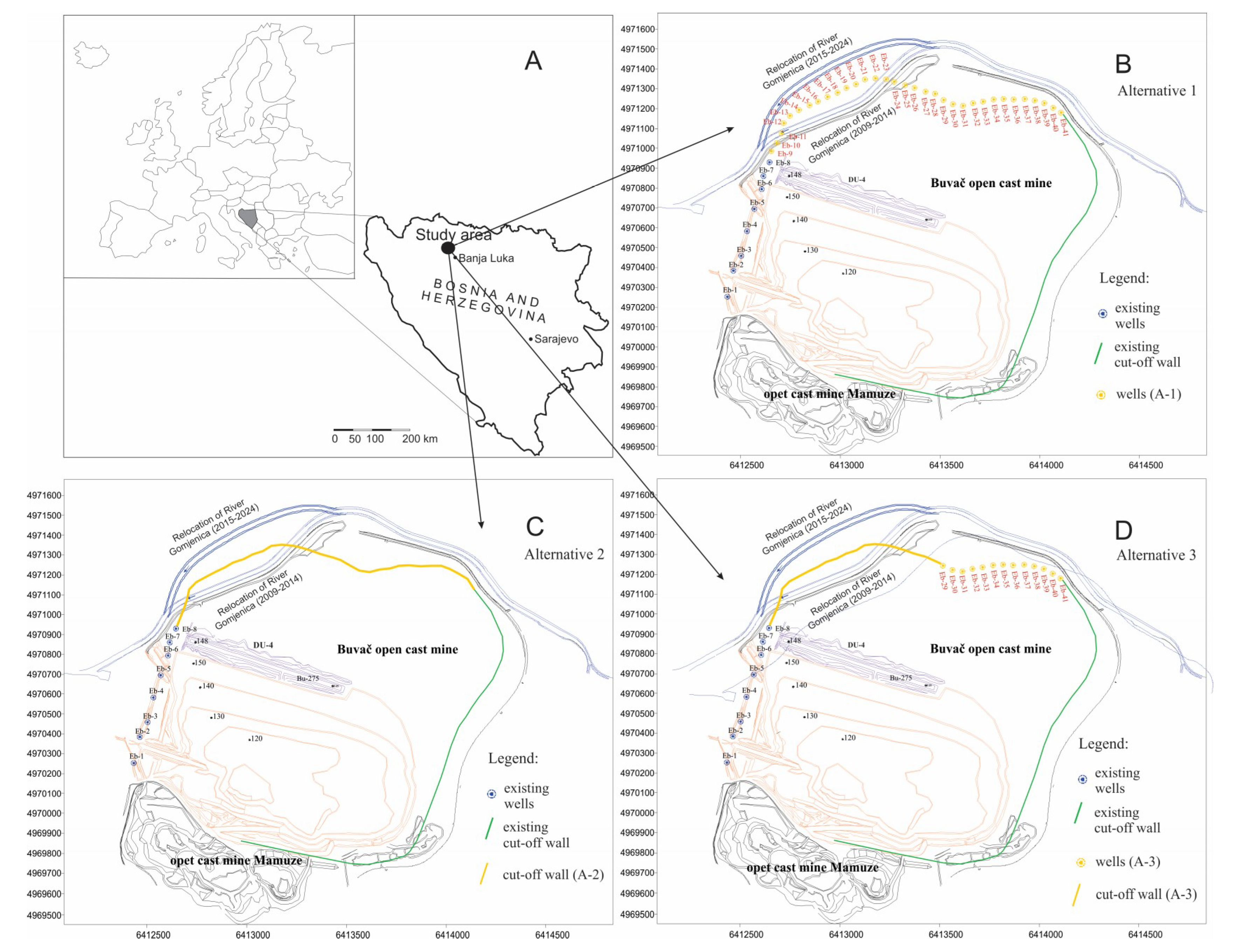
An open-cast mine is a suitable test site because of the complexity of both hydrogeologic conditions and the implementation of a proper groundwater control system. The Buvač limonite mine in Bosnia and Herzegovina was selected as the study area (Figure 1a). Based on numerical modeling, Polomčić & Bajić [1] discuss the design of groundwater control systems and describe three groundwater management scenarios (alternatives) for the Buvač open-cast mine, through to the projected cessation of mining operations (2024). They identify the groundwater control system components and portray their features, spatial distribution, construction sequence, and effectiveness of the entire system. The differences between the management scenarios originate from alluvial groundwater control solutions and components of the dewatering system (type, number and function). The configurations of all three alternatives included: eight drainage wells (blue dots in Figure 1) which drain the alluvial aquifer; a drainage ditch in the alluvial aquifer; a cut-off wall (green line in Figure 1); diverted river flow; and the locations, initial capacities, and lengths of operation of the drainage wells whose primarily function is to dewater the ore body. Common to all three alternatives is the fact that the groundwater level has to be a minimum of 15 m below the bench in the ore body. Based on the above, the problem is composed of three alternatives and four criteria: technical criterion, energy consumption, capital expenditure, and operating cost.

3.1. Alternative A1

In Alternative 1, the groundwater control system consists of 33 additional wells that tap the alluvial aquifer north of the open-cast mine (yellow dot in Figure 1b), whose overall capacity is 107 L/s. Plans called for the system to be commissioned on 1 January 2015.

3.2. Alternative A2

In Alternative 2, the groundwater control system consists of a cut-off wall in the alluvial aquifer, (rather than the 33 drainage wells), which is approximately 2000 m long and about 20 m deep on average (yellow line in Figure 1c). The cut-off wall was supposed to be completed on 1 January 2016.

3.3. Alternative A3

In Alternative 3, the groundwater control system is a combination of the above two scenarios (Figure 1d). In the northwestern part of the site, where the open-cast mine is closest to the river, a 1000 m long cut-off wall was assumed to be complete on 1 January 2016. Continuing from the wall, 13 drainage wells were assumed to have the same characteristics as in Scenario 1, but a total capacity of 65 L/s. These wells were to be placed online on 1 January 2017.

3.4. Technical Criterion (C1)

The technical criterion refers to the selection of the groundwater control system components, their advantages and disadvantages in terms of construction, and their performance relative to the local hydrogeology. It is also related to the possibility of modifying the technical features of the groundwater management system, or, in other words, shutting down a drainage well or changing its discharge capacity by means of different types of pumps. This criterion needs to be maximized.

3.5. Energy Consumption (C2)

Energy consumption refers to a set of measures whose objective is to optimize electric power consumption. Such measures should not affect the operation of the groundwater control system. They are contributors to energy security and consistent with environmental principles. The energy demand of wells is high and that of cut-off walls minimal. This criterion needs to be minimized.

3.6. Capital Expenditure (C3)

Capital expenditure refers to the overall cost of the groundwater control system components, their characteristics, number, ancillary equipment, and unit cost. This criterion needs to be minimized.

3.7. Operating Costs (C4)

Operating costs (CO) are related to labor costs and the costs of repair or replacement of groundwater control system components and equipment (periodic pump replacement or well rehabilitation), and monitoring.
There are many uncertainties inherent in operating costs over time. The ability to quantify them can significantly increase the reliability of the best alternative selection. The present paper applies a stochastic diffusion process called geometric Brownian motion, to model the flow of operating costs. A general Itô-Doob type stochastic differential equation takes the following form [49]:
d x t = ρ · ( x t , t ) d t + σ · ( x t , t ) · d W t ,   x t 0 = x 0
Here, t t 0 , Wt is the Brownian motion, and x t > 0 ; is the stochastic process. The following linear Itô-Doob type stochastic differential equation is used to describe the flow of operating costs:
d C O t = ρ · C O t d t + σ · C O t · d W t
where ρ is the drift, σ is the volatility and Wt is normalized Brownian motion. If the separation technique is applied, then Equation (16) becomes:
d C O t C O t = ρ · d t + σ · d W t
Let’s take the integration of both sides:
d C O t C O t = ( ρ · d t + σ · d W t ) d t
Obviously, the left side relates to the derivative of l n ( C O t ) . Applying the Itô calculus, we get the following equation:
l n ( d C O t C O t ) = ( ρ σ 2 2 ) Δ t + σ Δ t W t ,   W t ~ N ( 0 , 1 )
Finally, the analytical solution to Equation (16) is the geometric Brownian motion given by the following equation:
C O t = C O t 1 · e x p { ( ρ σ 2 2 ) Δ t + N ( 0 , 1 ) σ Δ t }
Equation (20) describes an operating cost scenario involving spot costs COt. Let C O = { C O t ,     t = 0 , 1 , , T } denote a cost scenario with spot costs COt, where COt is determined by Equation (20). 
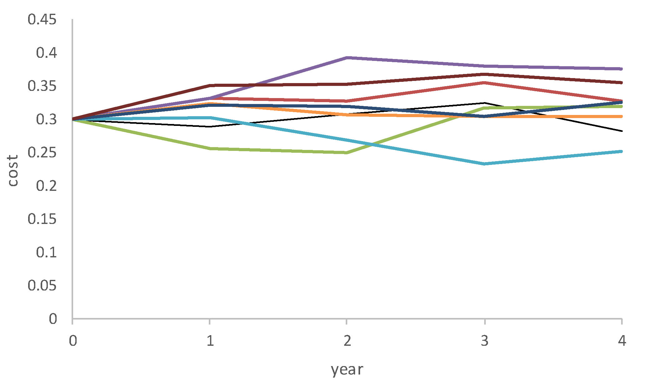
Figure 2 shows sample paths (s = 1, 2, ..., S) of the operating costs simulated using the above equation S times. This criterion needs to be minimized.

4. Decision-Making Model Using Simulation

The model is based on the ranking of proposed alternatives changing over a predefined timeframe and considers the variability of input parameters. By simulating a decision-making system, its action is mimicked in order to measure its response (output) to different inputs. The advantage of simulation is the possibility to replicate the evolution of a system as many times as necessary, under independent conditions. Simulation makes it possible for analysts to describe the uncertainty of variables that affect the ranking of projects at different times, depending on scenarios.
Criterion CO(t) has its own stochastic performance law described by geometric Brownian motion. Simulation provides the costs for every year of the proposed projects (i.e., project cost time-series).
Definition 1.
Let C O = [ c o i t ] m × T be a project cost matrix obtained for s = 1, where each row represents the cost path of the i-th project over the time horizon. The space of cost simulation is defined as follows:
C O s = [ [ c o i t ] m × T ] s = [ [ [ c o i t ] m × T ] 1 [ [ c o i t ] m × T ] 2 [ [ c o i t ] m × T ] 3 [ [ c o i t ] m × T ] s ] ,   s = 1 , 2 , , S
Definition 2.
According to the previous definition, let Y ˜ = [ [ D ˜ m n ] ] 1 × T be the dynamic decision-making matrix obtained for s = 1, where each element represents a decision-making matrix for every year. The space of the dynamic decision-making matrix simulation is defined as follows:
Y ˜ s = [ [ D ˜ m n ] ] s × t = [ [ [ D ˜ m n ] ] 11 [ [ D ˜ m n ] ] 12 [ [ D ˜ m n ] ] 1 t [ [ D ˜ m n ] ] 21 [ [ D ˜ m n ] ] 22 [ [ D ˜ m n ] ] 2 t [ [ D ˜ m n ] ] s 1 [ [ D ˜ m n ] ] s 2 [ [ D ˜ m n ] ] s t ] , s = 1 , , S ; t = 1 , , T
Definition 3.
Let A i = { A 1 , A 2 , , A m } be a set of proposed alternatives (projects) and Q i a g = { Q 1 a g , Q 2 a g , . . , Q m a g } a set of their defuzzified aggregated overall relative closeness values obtained for s = 1. Alternative Ai, which has the greatest aggregated overall relative closeness value, is the most suitable alternative and rank z = 1 is assigned to it (for example: A 2 = s u p { Q i = 1 , 2 , , m a g } z = 1 ). The remaining alternatives are ranked accordingly, in descending order of aggregated overall relative closeness values, and values 2, 3, …, m are assigned to them, respectively. If we take into consideration the number of simulations, then there are S rank orders of the given alternatives. The space of rank order simulation is defined as follows:
Z s = [ A 1 A 2 A m z 11 z 12 z 1 m z 21 z 22 z 2 m z s 1 z s 2 z s m ] ,   s = 1 , 2 , , S
The main goal of our model was to determine the best alternative with respect to the given criteria.
Definition 4.
Let Z = [ z s m ] S × m be a rank order matrix obtained by S simulations, and Ω = { Ω 1 , Ω 2 , , Ω m } = { s = 1 S z s 1 , s = 1 S z s 2 , , s = 1 S z s m } a set composed of column sums. The best alternative is defined as follows:
A b e s t = i n f { Ω }
and takes the rank of 1. The final ranking (FR) of the alternatives is formed according to the ascending order of the Ω set components.
F R = { i n f { Ω } , i n f { Ω m 1 } , i n f { Ω m 2 } , } = { 1 , 2 , 3 , , m }

5. Results and Discussion

As previously mentioned, the site on which the methodology was tested is the Buvač open-cast mine. Three groundwater control system alternatives and four criteria were analyzed in four-time slices (t = 1, t = 2, t = 3 and t = 4). The technical criterion was expressed through the AHPFAHP scale presented by Chang [50], Deng [51] and Tolga et al. [52]. The energy consumption criterion was given in kWh, while capital expenditure and operating costs were shown in euros. The input parameters for project evaluation are given in Table 1. Accordingly, based on Equations (15)–(20), Table 1 shows the spot value, drift and cost volatility parameters of Criterion 4 (operating costs). A total of 500 mathematical simulations were performed. The calculations were made in a special-purpose application based on Microsoft Excel.
One possible state of the C4 criterion (operating cost) over time is presented in Figure 3, while evaluations of information in different time episodes are shown in Table 2, Table 3, Table 4 and Table 5. The operating costs of Alternatives 1 and 3 vary over time considerably, given that the groundwater control system is comprised of 33 wells (Alternative 1) or 13 wells and a small impervious screen (Alternative 3). This means that systems made up of drainage wells are the most expensive option, because of the need for periodic pump replacement and well rehabilitation. This is not the case with the cut-off wall (Alternative 2). The operating costs of a groundwater control system comprised of a cut-off wall reflect solely maintenance labor.
Table 6 shows the calculated weights of the criteria in each time episode, taking into account the scores of the four criteria (technical criterion, energy consumption, capital expenditure and operating costs) by alternative (Table 1, Table 2, Table 3 and Table 4), based on Equations (1)–(6) from Section 2.
Based on Equations (7)–(11), the relative coefficient of closeness of the alternatives to the ideal solution in each time episode was calculated and is shown in Table 7.
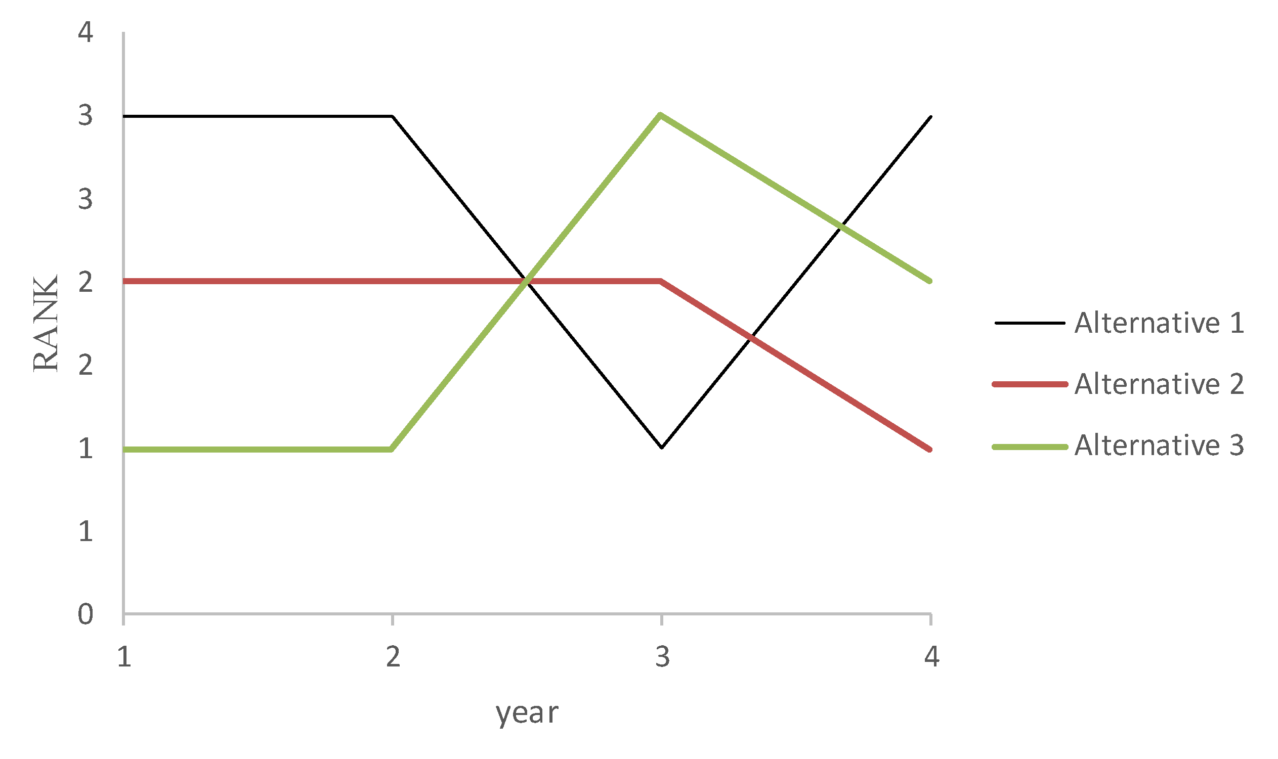
The performance ranking of alternatives in each time episode is shown in Table 8 and Figure 4. Applying the fuzzy TOPSIS method, the alternative that has the highest defuzzified value of the relative closeness coefficient is the optimal solution. For the first and second time intervals, the optimal solution is Alternative 3. In the third-time interval, the optimal solution is Alternative 1 and in the fourth-time interval Alternative 2.
Further, Table 9 shows the weight vector λ ˜ ( t ) = ( λ ˜ ( t 1 ) , λ ˜ ( t 2 ) , λ ˜ ( t 3 ) , λ ˜ ( t 4 ) ) obtained using Equation (14) and applying the proposed methodology.
The value of the aggregated overall relative closeness coefficient (AORC)— Q ˜ i a g ,   i = 1 ,   2 ,   3 and the rank of the i-th alternative in one simulation are shown in Table 10, along with the calculated values of the DAORC (defuzzified aggregated overall relative closeness coefficient). According to the methodology, the larger the defuzzified   Q ˜ i a g , the better the alternative. Consequently, Alternative 3 is the optimal solution.
Five hundred simulations were conducted using the proposed decision-making model (Section 4). A set of rankings was generated after the simulations (Table 11). As mentioned in Section 4, the alternatives were ultimately ranked according to the ascending order of the “Ω” set components. Based on the simulation results and Equation (25), the final ranking of the proposed alternatives is: A1(Ω3 = 1093), A2(Ω1 = 870) and A3(Ω2 = 1037). The lowest total score (sum) represented the optimal solution, meaning that Alternative 2 most often came first in the 500 simulations over time.

6. Conclusions

The paper proposed a dynamic multi-criteria decision-making model with real numbers and triangular fuzzy numbers, to deal with vagueness and uncertain information. The applied multi-criteria fuzzy-stochastic diffusion decision-making approach (fuzzy dynamic TOPSIS and geometric Brownian motion) is aimed at selecting the optimal alternatives, where different criteria generally have different representations, such as a real number and a fuzzy number.
The proposed concept was applied and tested on a groundwater management system in open-cast mining operations. The problem is highly complex because it is dynamic and involves continuous changes as the mining operations constantly expand. Thus, an efficient and flexible groundwater control system is required. Such problems indicate that the proposed criteria changeover a defined time horizon, so the dynamic multi-criteria decision-making method was tested.
The research implemented fuzzy multiple-criteria decision analysis in hydrogeology. It supported decision-making in connection with a problem that had several potential solutions and involved conflicting criteria. The optimal solution was selected after all the set criteria were assessed. The research highlights the need for an interdisciplinary approach, linking hydrogeology, hydrodynamics and groundwater management with other scientific disciplines, in addition to those mentioned in the paper: with fuzzy logic (mathematics and psychology) and multi-criteria decision analysis (decision theory).
Experiments showed that the proposed decision-making approach was able to select an optimal alternative effectively. Although the aim of the example provided here was to select an optimal groundwater control system, the proposed model can be applied in many different fields. The multi-criteria fuzzy-stochastic diffusion model presented for groundwater management can be used to solve hydrogeological and civil engineering problems related to the design and selection of optimal systems for water supply, irrigation, remediation of groundwater and soil pollution, and protection of urban areas, industrial zones, riparian lands, drained areas, and agglomerations.

Author Contributions

All the authors jointly contributed to the finalization of the paper: D.P. designed the numerical model and alternatives, Z.G. and D.B. performed the criterion analysis and conducted optimization calculations, and M.G. and M.N. carried out initial data analysis.

Funding

This research received no external funding.

Acknowledgments

We express our gratitude to the Serbian Ministry of Education, Science and Technological Development, for funding the projects: Potential and groundwork for sustainable use of groundwater (OI176022), Improvement of open-pit lignite mining technologies for better energy efficiency, security and safety at work (TR33039), and Simultaneous bioremediation and soilification of degraded areas with a view to conserving natural resources of biologically active substances and developing and producing biomaterials and dietary supplements (III43004). The authors also wish to thank the editors and three anonymous referees for their suggestions, which have helped us improve the quality and clarity of the paper.

Conflicts of Interest

On behalf of all the authors, the corresponding author states that there is no conflict of interest.

References

  1. Polomčić, D.; Bajić, D. Application of Groundwater modeling for designing a dewatering system: Case study of the Buvač Open Cast Mine, Bosnia and Herzegovina. Geol. Croat. 2015, 68, 123–137. [Google Scholar] [CrossRef]
  2. Hajkowicz, S.; Collins, K. A Review of Multiple Criteria Analysis for Water Resource Planning and Management. Water Resour. Manag. 2007, 21, 1553–1556. [Google Scholar] [CrossRef]
  3. Fernández-Pérez, Y.; Febles-Estrada, A.; Cruz, C.; Verdegay, J.L. Fuzzy Multi-criteria Decision Making Methods Applied to Usability Software Assessment: An Annotated Bibliography. In Complex Systems: Solutions and Challenges in Economics, Management and Engineering; Springer: Cham, Switzerland, 2018; pp. 165–189. [Google Scholar]
  4. Hafezalkotob, A.; Hafezalkotob, A.; Liao, H.; Herrera, F. An overview of MULTIMOORA for multi-criteria decision-making: Theory, developments, applications, and challenges. Inf. Fusion 2019, 51, 145–177. [Google Scholar] [CrossRef]
  5. Zarghami, M.; Szidarovszky, F. Stochastic-fuzzy multi criteria decision making for robust water resources management. Stoch. Environ. Res. Risk Assess. 2009, 23, 329–339. [Google Scholar] [CrossRef]
  6. Srdjevic, B.; Medeiros, Y.D.P. Fuzzy AHP Assessment of Water Management Plans. Water Resour. Manag. 2008, 22, 877–894. [Google Scholar] [CrossRef]
  7. Ghorbanzadeh, O.; Feizizadeh, B.; Blaschke, T. An interval matrix method used to optimize the decision matrix in AHP technique for land subsidence susceptibility mapping. Environ. Earth Sci. 2018, 77, 584. [Google Scholar] [CrossRef]
  8. Zhang, F.; Guo, S.; Ren, C.; Guo, P. Integrated IMO-TSP and AHP Method for Regional Water Allocation under Uncertainty. J. Water Resour. Plan. Manag. 2018. [Google Scholar] [CrossRef]
  9. Bajić, D.; Polomčić, D.; Ratković, J. Multi-criteria decision analysis for the purposes of groundwater control system design. Water Resour. Manag. 2017, 31, 4759–4784. [Google Scholar] [CrossRef]
  10. Sun, W.; Wang, X.; Wang, L.; Zhang, J.; Song, X. Multidisciplinary design optimization of tunnel boring machine considering both structure and control parameters under complex geological conditions. Struct. Multidiscip. Optim. 2016, 54, 1073–1092. [Google Scholar] [CrossRef]
  11. Golestanifar, M.; Ahangari, K. Choosing an optimal groundwater lowering technique for open pit mines. Mine Water Environ. 2012, 31, 192–198. [Google Scholar] [CrossRef]
  12. Aryafar, A.; Yousefi, S.; Doulati Ardejani, F. The weight of interaction of mining activities: Groundwater in environmental impact assessment using fuzzy analytical hierarchy process (FAHP). Environ. Earth Sci. 2013, 68, 2313–2324. [Google Scholar] [CrossRef]
  13. Li, L.; Shi, Z.H.; Yin, W.; Zhu, D.; Leung, N.G.S.; Cai, C.F.; Lei, A.L. A fuzzy analytic hierarchy process (FAHP) approach to eco-environmental vulnerability assessment for the Danjiangkou reservoir area, China. Ecol. Model. 2009, 220, 3439–3447. [Google Scholar] [CrossRef]
  14. Alizadeh, M.R.; Nikoo, M.R.; Rakhshandehroo, G.R. Hydro-environmental management of groundwater resources: A fuzzy-based multi-objective compromise approach. J. Hydrol. 2017, 551, 540–554. [Google Scholar] [CrossRef]
  15. Wu, Q.; Fan, Z.; Zhang, Z.; Zhou, W. Evaluation and zoning of groundwater hazards in Pingshuo No. 1 underground coal mine, Shanxi Province, China. Hydrogeol. J. 2014, 22, 1693–1705. [Google Scholar] [CrossRef]
  16. Jha, M.K.; Chowdary, V.M.; Chowdhury, A. Groundwater assessment in Salboni Block, West Bengal (India) using remote sensing, geographical information system and multi-criteria decision analysis techniques. Hydrogeol. J. 2010, 18, 1713–1728. [Google Scholar] [CrossRef]
  17. Levy, K.J. Multiple criteria decision making and decision support systems for flood risk management. Stoch. Environ. Res. Risk Assess. 2005, 19, 438–448. [Google Scholar] [CrossRef]
  18. Choubin, B.; Rahmati, O.; Tahmasebipour, N.; Feizizadeh, B.; Pourghasemi, H.R. Application of Fuzzy Analytical Network Process Model for Analyzing the Gully Erosion Susceptibility. In Natural Hazards GIS-Based Spatial Modeling Using Data Mining Techniques; Pourghasemi, H., Rossi, M., Eds.; Advances in Natural and Technological Hazards Research; Springer: Cham, Switzerland, 2019; Volume 48. [Google Scholar]
  19. Ghorbanzadeh, O.; Feizizadeh, B.; Blaschke, T. Multi-criteria risk evaluation by integrating an analytical network process approach into GIS-based sensitivity and uncertainty analyses. Geomat. Nat. Hazards Risk 2017, 9, 127–151. [Google Scholar] [CrossRef] [Green Version]
  20. Roozbahani, A.; Zahraie, B.; Tabesh, M. PROMETHEE with Precedence Order in the Criteria (PPOC) as a New Group Decision Making Aid: An Application in Urban Water Supply Management. Water Resour. Manag. 2012, 26, 3581–3599. [Google Scholar] [CrossRef]
  21. Afshar, A.; Mariño, M.A.; Saadatpour, M. Fuzzy TOPSIS Multi-Criteria Decision Analysis Applied to Karun Reservoirs System. Water Resour. Manag. 2011, 25, 545–563. [Google Scholar] [CrossRef]
  22. Onu, U.; Xie, Q.; Xu, L. A Fuzzy TOPSIS model Framework for Ranking Sustainable Water Supply Alternatives. Water Resour. Manag. 2017, 31, 2579–2593. [Google Scholar] [CrossRef]
  23. Senent-Aparicio, J.; Pérez-Sánchez, J.; Carrillo-García, J.; Soto, J. Using SWAT and Fuzzy TOPSIS to Assess the Impact of Climate Change in the Headwaters of the Segura River Basin (SE Spain). Water 2017, 9, 149. [Google Scholar] [CrossRef]
  24. Campanella, G.; Ribeiro, R.A. A framework for dynamic multiple-criteria decision making. Decis. Support Syst. 2011, 52, 52–60. [Google Scholar] [CrossRef]
  25. Jassbi, J.J.; Ribeiro, R.A.; Varela, L.R. Dynamic MCDM with future knowledge for supplier selection. J. Decis. Syst. 2014, 23, 232–248. [Google Scholar] [CrossRef]
  26. Keshavarz-Ghorabaee, M.; Amiri, M.; Zavadskas, E.K.; Turskis, Z.; Antucheviciene, J. A Dynamic Fuzzy Approach Based on the EDAS Method for Multi-Criteria Subcontractor Evaluation. Information 2018, 9, 68. [Google Scholar] [CrossRef]
  27. Yu, P.L.; Chen, Y.C. Dynamic MCDM, Habitual Domains and Competence Set Analysis for Effective Decision Making in Changeable Spaces. In Trends in Multiple Criteria Decision Analysis; Ehrgott, M., Figueira, J.R., Greco, S., Eds.; Springer: Boston, MA, USA, 2010; pp. 1–35. [Google Scholar] [CrossRef]
  28. Ziemba, P.; Jankowski, J.; Wątróbski, J. Dynamic Decision Support in the Internet Marketing Management. In Transactions on Computational Collective Intelligence XXIX; Nguyen, N.T., Kowalczyk, R., Eds.; Springer International Publishing: Cham, Switzerland, 2018; pp. 39–68. [Google Scholar] [CrossRef]
  29. Hashemkhani Zolfani, S.; Maknoon, R.; Zavadskas, E.K. An introduction to Prospective Multiple Attribute Decision Making (PMADM). Technol. Econ. Dev. Econ. 2016, 22, 309–326. [Google Scholar] [CrossRef]
  30. Chen, Y.; Li, K.W.; He, S. Dynamic multiple criteria decision analysis with application in emergency management assessment. In Proceedings of the IEEE International Conference on Systems, Man and Cybernetics (SMC), Istanbul, Turkey, 10–13 October 2010; pp. 3513–3517. [Google Scholar] [CrossRef]
  31. Zulueta, Y.; Martell, V.; Martinez, J.; Martinez, L. A Dynamic Multi-Expert Multi-Criteria Decision Making Model for Risk Analysis. In MICAI 2013, Part I, LNAI, Volume 8265; Castro, F., Gelbukh, A., Gonzalez, M., Eds.; Springer: Berlin, Germany, 2013; pp. 132–143. [Google Scholar] [CrossRef]
  32. Shannon, C.E.; Weaver, V. The Mathematical Theory and Communication; The University of Illinois Press: Urbana, IL, USA, 1947. [Google Scholar]
  33. Zeleney, M. Multiple Criteria Decision Making; McGraw Hill: New York, NY, USA, 1982. [Google Scholar]
  34. Hwang, C.L.; Yoon, K. Multiple Attribute Decision Making-Methods and Applications, a State of the Art Survey; Springer: New York, NY, USA, 1981. [Google Scholar]
  35. Wang, Y.M.; Elhag, T.M.S. Fuzzy TOPSIS method based on alpha level sets with an application to bridge risk assessment. Expert Syst. Appl. 2006, 31, 309–319. [Google Scholar] [CrossRef]
  36. Zeng, S.; Hussain, A.; Mahmood, T.; Irfan Ali, M.; Ashraf, S.; Munir, M. Covering-Based Spherical Fuzzy Rough Set Model Hybrid with TOPSIS for Multi-Attribute Decision-Making. Symmetry 2019, 11, 547. [Google Scholar] [CrossRef]
  37. Ziemba, P.; Jankowski, J.; Wątróbski, J. Online Comparison System with Certain and Uncertain Criteria Based on Multi-criteria Decision Analysis Method. In Computational Collective Intelligence; Nguyen, N.T., Papadopoulos, G.A., Jędrzejowicz, P., Trawiński, B., Vossen, G., Eds.; Springer International Publishing: Cham, Switzerland, 2017; pp. 579–589. [Google Scholar] [CrossRef]
  38. Chou, Y.-C.; Yen, H.-Y.; Dang, V.T.; Sun, C.-C. Assessing the Human Resource in Science and Technology for Asian Countries: Application of Fuzzy AHP and Fuzzy TOPSIS. Symmetry 2019, 11, 251. [Google Scholar] [CrossRef]
  39. Solangi, Y.A.; Tan, Q.; Khan, M.W.A.; Mirjat, N.H.; Ahmed, I. The Selection of Wind Power Project Location in the Southeastern Corridor of Pakistan: A Factor Analysis, AHP, and Fuzzy-TOPSIS Application. Energies 2018, 11, 1940. [Google Scholar] [CrossRef]
  40. Kim, T.H.; Kim, B.; Han, K.-Y. Application of Fuzzy TOPSIS to Flood Hazard Mapping for Levee Failure. Water 2019, 11, 592. [Google Scholar] [CrossRef]
  41. Koulinas, G.; Demesouka, O.; Marhavilas, P.; Vavatsikos, A.; Koulouriotis, D. Risk Assessment Using Fuzzy TOPSIS and PRAT for Sustainable Engineering Projects. Sustainability 2019, 11, 615. [Google Scholar] [CrossRef]
  42. Kannchen, M.; Ziemba, P.; Borawski, M. Use of the PVM Method Computed in Vector Space of Increments in Decision Aiding Related to Urban Development. Symmetry 2019, 11, 446. [Google Scholar] [CrossRef]
  43. Chen, C.T. Extension of the TOPSIS for group decision making under fuzzy environment. Fuzzy Sets Syst. 2000, 114, 1–9. [Google Scholar] [CrossRef]
  44. Chu, T.C. Selecting plant location via a fuzzy TOPSIS approach. Int. J. Adv. Manuf. Technol. 2002, 20, 859–864. [Google Scholar] [CrossRef]
  45. Yang, T.; Hung, C.C. Multiple-attribute decision making methods for plant layout design problem. Robot. Comput. Integr. Manuf. 2007, 23, 126–137. [Google Scholar] [CrossRef]
  46. Gligorić, Z.; Gligorić, M. Model of strategic decision making in mining industry based on fuzzy dynamic TOPSIS method. J. Multidiscip. Eng. Sci. Technol. 2015, 3, 470–475. [Google Scholar]
  47. Vinodh, S.; Sai Balagi, T.S.; Patil, A. A hybrid MCDM approach for agile concept selection using fuzzy DEMATEL, fuzzy ANP and fuzzy TOPSIS. Int. J. Adv. Manuf. Technol. 2016, 83, 1979–1987. [Google Scholar] [CrossRef]
  48. Zhang, Z. An Approach to Dynamic Multi-attribute Decision Making for Choosing Green Supplier. J. Converg. Inf. Technol. 2012, 7, 261–269. [Google Scholar] [CrossRef]
  49. Ladde, G.S.; Sambandham, M. Stochastic Versus Deterministic Systems of Differential Equations; Marcel Dekker, Inc.: New York, NY, USA, 2004. [Google Scholar]
  50. Chang, D.Y. Applications of the extent analysis method on fuzzy AHP. Eur. J. Oper. Res. 1996, 95, 649–655. [Google Scholar] [CrossRef]
  51. Deng, H. Multicriteria analysis with fuzzy pair-wise comparison. Int. J. Approx. Reason. 1999, 21, 215–231. [Google Scholar] [CrossRef]
  52. Tolga, E.; Demircan, M.; Kahraman, C. Operating system selection using fuzzy replacement analysis and analytic hierarchy process. Int. J. Prod. Econ. 2005, 97, 89–117. [Google Scholar] [CrossRef]
Figure 1. Study area (A) and dewatering systems: Alternative 1 (B). Alternative 2 (C), and Alternative 3 (D) (Bajić et al. [9]; modified).
Symmetry 11 00705 g001
Figure 2. Simulated operating cost paths on an annual time scale.
Symmetry 11 00705 g002
Figure 3. A simulation of operating cost paths.
Symmetry 11 00705 g003
Figure 4. Ranking of alternatives over time.
Symmetry 11 00705 g004
Table 1. Input parameters.
AlternativeCriterionValue
A1C1max (FAHP Scale)(t = 1) = (1, 1, 1); (t = 2) = (1.5, 2, 2.5); (t = 3) = (0.666,1,1.5); (t = 4) = (0.666, 1, 1.5)
C2min (×106 kWh)(t = 1) = 1.445; (t = 2) = 5.913; (t = 3) = 6.044; (t = 4) = 5.913
C3min (×106 Euro)(t = 1) = 0.1193; (t = 2) = 1.8351; (t = 3) = 0.2410; (t = 4) = 0.0000
C4min (×106 Euro)spot value 0.30; drift 0.0291; cost volatility rate 0.0799
A2C1max (FAHP Scale)(t = 1) = (1, 1, 1); (t = 2) = (0.666, 1, 1.5); (t = 3) = (3.5, 4, 4.5); (t = 4) = (3.5, 4, 4.5)
C2min (×106 kWh)(t = 1) = 1.445; (t = 2) = 1.576; (t = 3) = 1.078; (t = 4) = 1.578
C3min (×106 Euro)(t = 1) = 0.1193; (t = 2) = 0.7094; (t = 3) = 9.4490; (t = 4) = 0.0000
C4min (×106 Euro)spot value 0.30; drift 0.0014; cost volatility rate 0.0258
A3C1max (FAHP Scale)(t = 1) = (1, 1, 1); (t = 2) = (0.666, 1, 1.5); (t = 3) = (2, 3, 3.5); (t = 4) = (2.5, 3, 3.5)
C2min (×106 kWh)(t = 1) = 1.445; (t = 2) = 1.576; (t = 3) = 3.416; (t = 4) = 3.285
C3min (×106 Euro)(t = 1) = 0.1193; (t = 2) = 0.7094; (t = 3) = 7.8848; (t = 4) = 0.0000
C4min (×106 Euro)spot value 0.30; drift 0,0142; cost volatility rate 0.0512
Time slice 4 years
Interval 1 year
Sample 500 simulations
Table 2. Information for t = 1.
Criterion C1 C2C3C4
Alternativea1b1c1
A11111.4450.11940.3352
A21111.4450.11940.3031
A31111.4450.11940.296
Table 3. Information for t = 2.
Criterion C1 C2C3C4
Alternativea1b1c1
A11.522.55.9131.83510.3213
A20.66611.51.5770.70950.3063
A30.66611.51.5770.70950.3012
Table 4. Information for t = 3.
Criterion C1 C2C3C4
Alternativea1b1c1
A10.66611.56.0440.24100.2975
A23.544.51.0789.44900.3102
A3233.53.4167.88490.3132
Table 5. Information for t = 4.
Criterion C1 C2C3C4
Alternativea1b1c1
A10.66611.55.91300.307
A23.544.51.578600.32
A32.533.53.28500.3366
Table 6. Weights of criteria in time interval.
Timet1t2t3t4
a1b1c1a2b2c2a3b3c3a4b4c4
C10000.566930.154120.364840.273220.190510.295780.498940.495650.67533
C20000.380140.553320.331110.243580.277960.24790.393540.501510.43985
C30000.200310.291570.174480.465460.531150.4737000
C41110.000680.000990.00590.000330.000380.000340.000220.002850.0025
Table 7. Relative closeness coefficient in time interval.
Timet1t2t3t4
Alternativea1b1c1a2b2c2a3b3c3a4b4c4
A10000.566930.154120.364840.273220.190510.295780.498940.495650.67533
A20.819210.819210.819210.380140.553320.331110.243580.277960.24790.393540.501510.43985
A31110.200310.291570.174480.465460.531150.47370.123130.17410.32331
Table 8. Ranking in time interval.
Timet1t2t3t4
AlternativeDCRankDCRankDCRankDCRank
A1030.3376130.6083710.181913
A20.8192120.6242920.3829820.727251
A3110.6242910.3166130.513492
Table 9. Weight vector in time interval.
Timet1t2t3t4
a1b1c1a2b2c2a3b3c3a4b4c4
λ(t)0.495410.487820.505200.132160.142300.125150.117640.132310.117930.235420.237740.27149
Table 10. Aggregated overall relative closeness coefficient and rank (s = 1).
AlternativeAORCDAORCRank
a1b1c1
A10.116570.103080.194740.138133
A20.537040.636220.669780.614352
A30.607600.692330.717250.672391
Table 11. Simulations.
SimulationRank
A1A2A3
1132
2123
3312
4132
5321
6231
7123
8312
9132
10312
495132
496123
497321
498123
499312
500312
Sum10938701037

