Abstract
Imprecise constrained matrix games (such as fuzzy constrained matrix games, interval-valued constrained matrix games, and rough constrained matrix games) have attracted considerable research interest. This article is concerned with developing an effective fuzzy multi-objective programming algorithm to solve constraint matrix games with payoffs of fuzzy rough numbers (FRNs). For simplicity, we refer to this problem as fuzzy rough constrained matrix games. To the best of our knowledge, there are no previous studies that solve the fuzzy rough constrained matrix games. In the proposed algorithm, it is proven that a constrained matrix game with fuzzy rough payoffs has a fuzzy rough-type game value. Moreover, this article constructs four multi-objective linear programming problems. These problems are used to obtain the lower and upper bounds of the fuzzy rough game value and the corresponding optimal strategies of each player in any fuzzy rough constrained matrix games. Finally, a real example of the market share game problem demonstrates the effectiveness and reasonableness of the proposed algorithm. Additionally, the results of the numerical example are compared with the GAMS software results. The significant contribution of this article is that it deals with constraint matrix games using two types of uncertainties, and, thus, the process of decision-making is more flexible.
1. Introduction
Different types of uncertainty (such as fuzziness, randomness, ambiguity, roughness) are common in many real-life decision-making problems, including matrix games. Determining how to represent uncertain information is one of the most critical issues among other uncertainty-related problems. However, decision-makers might face hybrid uncertain scenarios where roughness and fuzziness exist simultaneously. In such scenarios, fuzzy rough numbers (FRNs) are used to model the decision-making problem. Roughness and fuzziness play a significant role among types of uncertainty problems. Dubois and Prade [1] discussed the fuzzification of rough sets. Moreover, Morsi and Yakout [2] defined the lower and upper approximations of the fuzzy rough sets. Rough programming and fuzzy programming have been proposed for decision-making problems under uncertainty. In these decision-making problems, fuzziness and roughness are considered separate aspects. Several researchers have studied the issue of combining roughness and fuzziness in a general framework for the study of fuzzy rough sets. Recently, the fuzzy rough set has been considered in several practical problems. As an illustration, Wang [3] studied the mining of stock price by using a fuzzy rough set system. Shen et al. [4] adopted a fuzzy rough estimator to study algae populations models, given specific water characteristics. Additionally, the false-negative and false-positive effects on network attacks have been examined by Yilun Shang [5]. Bhatt et al. [6] proposed a fuzzy rough set algorithm for feature selection. Furthermore, Liu et al. [7] introduced some properties and definitions of fuzzy rough numbers. Liu et al. [8] studied a fuzzy rough set for the task of scheduling models. Finally, Yilun Shang [9] studied the robustness of scale-free networks under attack with tunable grey information.
Game theory is a mathematical tool to study the conflict and cooperation among intelligent, rational decision-makers. It has many applications in specialized fields such as finance, strategic welfares, management problems, political voting systems, economic auctions, social problems, and military issues [10,11,12,13]. Because of the imprecision or lack of the available information in real game theory, the players can only estimate the payoff value with some imprecise degree. In order to make the constrained matrix game more applicable to real competitive decision-making problems, fuzzy rough numbers [1] have been applied to describe uncertain and imprecise information appearing in the constrained matrix game. The fuzzy rough game theory provides an efficient framework which solves real-life cooperative and conflict problems with fuzzy rough information. It is an interesting research field not only for mathematicians but also for biologists, behavioral scientists, economists, medical doctors, environmentalists, and pattern recognizers.
In recent years, many research articles examined imprecise matrix games; for example, linear programming has been adopted to solve the zero-sum two-person game with payoffs of grey numbers [14]. Ammar et al. [15] studied constraint matrix games with rough interval payoffs. Bector et al. [16] studied the duality fuzzy linear programming for matrix games with fuzzy payoffs and fuzzy goals. Takahashi [17] analyzed the zero-sum two-person matrix game under random environment. Chunqiao Tan et al. [18] studied Bertrand game in a fuzzy number environment. Jana et al. [19] examined the solution of matrix games with generalized trapezoidal fuzzy payoffs. Prasanta Mula et al. [20] proposed a bi-rough programming algorithm for solving bi-matrix games with bi-rough payoffs. Li and Nan [21] studied imprecise matrix games in a triangular intuitionistic fuzzy environment. Jiang-Xia Nan et al. [22] studied constraint matrix games with interval payoffs. Deng-Feng Li et al. [23] analyzed an alfa-cut linear programming algorithm for solving fuzzy constrained matrix games. Also, Roy [24] discussed the game theory with the fuzzy set theory and multi-criteria decision-making. Jana et al. [25] considered dual hesitant fuzzy matrix games based on a new similarity measure. Aggarwal et al. [26] discussed the solution of matrix game with I-fuzzy payoffs. Bhaumik et al. [27] developed a robust ranking algorithm to solve matrix game with Atanassov’s intuitionistic fuzzy payoffs. Roy et al. [28] studied intelligent water management with a triangular type-2 intuitionistic fuzzy matrix games approach.
In this article, we propose a novel algorithm for solving fuzzy rough constrained matrix games. The lower and upper bounds of the fuzzy rough game value of any fuzzy rough constrained matrix games can be determined by solving the four multi-objective linear programming models as shown in Equations (13)–(16). These multi-objective models can be solved using any of the known multi-objective optimization algorithms, such as goal programming, interactive approaches, fuzzy programming, and utility theory [29,30]. However, in this article, we develop a fuzzy multi-objective programming algorithm using Zimmermann’s fuzzy programming algorithm [31].
The main contributions of this article are summarized as follows:
- Developing a new type of constraint matrix games with payoffs of fuzzy rough numbers.
- Constructing fuzzy models from the proposed fuzzy rough models.
- Solving the derived multi-objective models using Zimmermann’s programming approach [31].
- Solving the reduced crisp models using LINGO-14.0 (Lindo Systems, Chicago, IL, USA).
- Demonstrating the models and algorithm with the help of a real example of the market share game problem [32], obtaining optimal strategies.
The remainder of this article is organized as follows: Section 2 introduces some essential definitions such as triangular fuzzy variables, rough variables, and fuzzy rough variables. Section 3 presents the classical constrained matrix games and their properties. Constrained matrix game with payoffs of FRNs and Zimmermann method for solving fuzzy multi-objective programming models are introduced in Section 4. Section 5 presents a numerical experiment of the market share problem that demonstrates the applicability and validity of the proposed algorithm and models. Finally, Section 6 presents the conclusions of this work.
2. Preliminaries
Here, we include some properties and concepts of fuzzy variables, rough variables, and fuzzy rough variables, which are applied in the following sections.
2.1. Triangular Fuzzy Number TFNs
Definition 1
[31] (p. 11): A fuzzy set , defined on the universal set Y is the family , where is the membership function such that if y does not belong to , if y strictly belongs to .
Definition 2
[31] (p. 14): The support of , represented by , is the set of points at which is positive.
Definition 3
[31] (p. 14): is normal if there is such that .
Definition 4
[33] (p. 23): Let R be the real numbers set, the fuzzy number is a mapping, with the following properties.
- (1)
- is the upper semi continuous membership function,
- (2)
- is the convex fuzzy set, i.e.,for all
- (3)
- is normal,
- (4)
- is a support of .
Definition 5
[33] (p. 24): A fuzzy number is said to be a triangular fuzzy number if its membership function is defined as follows:
where is the mean of , and and are the upper and lower limits of , respectively. If then TFN is reduced to a real number.
Definition 6
[33] (p. 24): The -cut set of the triangular fuzzy number is defined as , where . Thus, for any , we can obtain an -cut set of the triangular fuzzy number , which is an interval, denoted by .
Corollary 1
[34] (p. 374): Let and be any two triangular fuzzy numbers. Then, their arithmetical operations can be represented as follows:
where is any real number.
Definition 7
[34] (p. 374): Let and be two triangular fuzzy numbers. Then, if, and only if, , , and . Similarly, if, and only if, , , and .
Definition 8
[34] (p. 375): Let be any triangular fuzzy number. The maximization triangular fuzzy numbers problem is represented as follows:
which is equivalent to the multi-objective mathematical programming problem as follows:
where is the triangular fuzzy numbers set, and is the constraints set.
Definition 9
[34] (p. 375): Let be any triangular fuzzy number. The minimization triangular fuzzy numbers problem is represented as follows:
which is equivalent to the multi-objective mathematical programming model, as follows:
where is the constraints set.
2.2. Rough Interval
Definition 10
[35] (p. 342): Let be the universal set, be the equivalence relation on , be the equivalence class set of , and be a nonempty subset of . The lower and upper approximations of the set are defined as
If , then set is called rough set.
Definition 11
[36] (p. 487): The qualitative value is called a rough interval (RI) when one can assign two closed intervals and on a real number set to it, where . Moreover,
- (i)
- If , then surely takes y (denoted by ).
- (ii)
- If , then possibly takes y.
- (iii)
- If , then surely does not take y (denoted by ).
and are called the upper approximation interval and lower approximation interval of , respectively. Further, is denoted by .
Definition 12
[37] (p. 677): Let * be a binary operation on rough intervals. For two rough intervals number and , when and , we have:
If
Then
Definition 13
[38] (p. 1700): Let be a rough value. Then, the lower trust measure of the rough event is defined by , where Card () represents the cardinal number. Similarly, the upper trust measure is defined by
The trust measure of the rough event is defined by
Definition 14
[38] (p. 1700): Let be a rough interval (RI) such that gefh, then the trust measure of a rough event is defined as
and the - pessimistic value of is
Theorem 1
[7] (p. 95): Let , where is a RI. Then the expected value of is .
2.3. Fuzzy Rough Number
Definition 15
[39] (p. 2102): Let Z denote a compact real numbers set. A fuzzy rough variable is defined as , where and are fuzzy numbers called lower and upper approximation fuzzy numbers of with . Supposing , we can write , , where are triangular fuzzy numbers defined as:
, , , and where and
Definition 16
[39] (p. 2103): For the fuzzy rough , the following holds:
- i.
- iff and
- ii.
- iff and .
Definition 17
[39] (p. 2103): A fuzzy rough interval is said to be normalized if and are normal.
Definition 18
[39] (p. 2103): Let and be two fuzzy rough intervals in R. We write if, and only if, and
Definition 19
[39] (p. 2104): The -cut set of a fuzzy rough interval is defined as: , where are intervals with .
Definition 20
[39] (p. 2104): For any two fuzzy rough intervals and , when and , the operation for fuzzy rough numbers can be written as follows:
3. The Classical Constraint Matrix Games
In this Section, a review of the classical constraint matrix games [40] is presented. Let and be sets of pure strategies for each player. The player I’s payoff matrix can be represented as . The mixed strategies vectors are expressed as and . Players I and II respectively must select their mixed strategies and from convex polyhedrons, which are defined as constrained sets determined by some inequalities and equations. Let be player I’s strategy constrained set, where , , and c is a positive integer. Let be player II’s strategy constrained set, where , , and d is a positive integer. Note that includes , since is equivalent to both and . Similarly, includes .
Thus, a constrained matrix game A means that player I’s payoff matrix is A, and player II’s payoff matrix is −A, and the strategies’ constrained sets for player I and II are P and Q, respectively.
Suppose that players I and II, respectively, select their optimal strategies from the constrained sets P and Q in order to maximize their payoffs, then player I’s expected payoff can be represented as follows:
Thus, player I will select strategy that satisfies
where u is player I’s gain-floor.
Similarly, player II chooses strategy that satisfies
where v is the player II’s loss-ceiling
Definition 21
[40]: If and , the following conditions are satisfied:
Then, is called the saddle point, and is called the game value of the constrained matrix game A.
Theorem 2
[40]: If and are feasible solutions of the two linear programming problems as follows:
and
respectively. Then, is the saddle point, and is the game value of the constrained matrix game A.
Theorem 3
[40]: If there exists , where , so that
for all , then is the saddle point, and is the game value of the constrained matrix game A.
4. Fuzzy Rough Constraint Matrix Games and Solutions Algorithm
4.1. Fuzzy Rough Constraint Matrix Games
The constrained matrix game problem has been extensively studied in the literature in uncertain environments [22,23]. However, in some real situations, a single uncertain environment (such as rough, fuzzy, stochastic, etc.) is not enough to tackle the situation. In such situations, one can introduce a constrained matrix game with payoffs of fuzzy rough numbers (hybrids of a fuzzy variable with a rough variable). Let us consider a constrained matrix game with FRNs payoffs, where mixed strategy and would be fuzzy rough sets on and . The fuzzy rough payoff matrix of player I is expressed as , where each is a fuzzy rough number, . and represent the fuzzy rough constraint sets of strategies for player I and II, where and are vectors of fuzzy rough numbers, and and are fuzzy rough matrixes, with , , , and
Then, a constrained matrix game with payoffs of fuzzy rough numbers and sets of strategies and being fuzzy rough constraint sets is simply called a fuzzy rough constrained matrix game.
Thus, Equations (5) and (6) can be expressed in the following corresponding fuzzy rough mathematical programming models as follows:
and
If is the optimal solution of Equation (7), is called an optimal strategy of player I in the fuzzy rough constraint matrix game. Likewise, if is the optimal solution of Equation (8), is called an optimal strategy of player II in the fuzzy rough constraint matrix game, and is called a solution of the fuzzy rough constraint matrix game. Denote
and
Then, and are called player II’s loss-ceiling and player I’s gain-floor, respectively.
Theorem 4:
Suppose that and are the optimal solutions of Equation (7) and (8), respectively. Denote and . Then, and are fuzzy rough numbers.
We follow the method introduced in [39] to convert fuzzy rough mathematical programming problems (Equations (7) and (8)) into general fuzzy mathematical programming problems as follows:
and
Equations (9)–(12) are fuzzy mathematical programming models. According to Corollary 1 and Definition 8 or Definition 9, Equations (9)–(12) can be transformed into the multi-objective linear programming models as follows:
where ,
where
where and
where .
4.2. Zimmermann’s Algorithm
In this Subsection, we introduce a fuzzy multi-objective programming algorithm to solve Equations (13)–(16) by using Zimmermann’s fuzzy programming algorithm [31].
Firstly, we determine the negative and positive ideal solutions of Equation (13) by solving three mathematical programming problems with three different objective functions. Using the simplex technique of linear programming problem, we solve the mathematical programming problem as follows:
denoting its optimal solution by and its optimal objective value by
Analogously, according to Equation (13), we solve the mathematical programming problem using the simplex technique as follows:
denoting its optimal solution by and its optimal objective value by
Analogously, according to Equation (13), we solve the mathematical programming problem using the simplex technique as follows:
denoting its optimal solution by and its optimal objective value by
Therefore, the positive ideal solution of Equation (13) can be represented as The negative ideal solution of Equation (13) can be expressed as follows:
and
The relative membership functions of the three objective functions in Equation (13) can be computed as follows:
and
Using Zimmermann’s algorithm [31], Equation (13) is transformed into the linear programming problem as follows:
solving Equation (20) by using the simplex technique, we obtain the lower bound gain-floor and the optimal strategy for player I.
In the same analysis of Equation (13), according to Equation (14), we solve the mathematical programming problem using the simplex technique as follows:
denoting its optimal solution by and its optimal objective value by
Analogously, according to Equation (14), we solve the mathematical programming problem using the simplex technique as follows:
denoting its optimal solution by and its optimal objective value by
Analogously, according to Equation (14), we solve the mathematical programming problem using the simplex technique as follows:
denoting its optimal solution by and its optimal objective value is denoted by
Thus, the positive ideal solution of Equation (14) can be represented as The negative ideal solution of Equation (14) can be obtained as follows:
and
The relative membership functions of the three objective functions in Equation (14) can be expressed as follows:
and
Using Zimmermann’s algorithm [31], Equation (14) is transformed into the linear programming problem as follows:
Solving Equation (24) by using the simplex technique, we obtain the upper bound gain-floor and the optimal strategy for player I.
In the same analysis of Equation (14), according to Equation (15), we solve the mathematical programming problem using the simplex technique as follows:
denoting its optimal solution by and its optimal objective value by
Analogously, according to Equation (15), we solve the mathematical programming problem using the simplex technique as follows:
denoting its optimal solution by and its optimal objective value by
Analogously, according to Equation (15), we solve the mathematical programming problem using the simplex technique as follows:
denoting its optimal solution by and its optimal objective value by
Thus, the positive ideal solution of Equation (15) can be represented as The negative ideal solution of Equation (15) can be constructed as follows:
and
The relative membership functions of the three objective functions in Equation (15) can be formulated as follows:
and
Using Zimmermann’s algorithm [31], Equation (15) is transformed into the linear programming problem as follows:
solving Equation (28) by using the simplex technique, we obtain the lower bound loss-ceiling and the optimal strategy for player II.
Similarly, according to Equation (16), we solve the mathematical programming problem using the simplex technique as follows:
denoting its optimal solution by and its optimal objective value by
Analogously, according to Equation (16), we solve the mathematical programming problem using the simplex technique as follows:
denoting its optimal solution by and its optimal objective value by
Analogously, according to Equation (16), we solve the mathematical programming problem using the simplex technique as follows:
denoting its optimal solution by and its optimal objective value by
Thus, the positive ideal solution of Equation (16) can be computed as The negative ideal solution of Equation (16) can be expressed as follows:
and
The relative membership functions of the three objective functions in Equation (16) can be obtained as follows:
and
Using Zimmermann’s algorithm [31], Equation (16) is transformed into the linear programming problem as follows:
solving Equation (32) by using the simplex technique, we obtain the upper bound loss-ceiling and the optimal strategy for player II.
4.3. Solution Methodology
On the basis of the discussion mentioned above, the algorithm for solving fuzzy rough constrained matrix game can be summarized as follows (Figure 1).
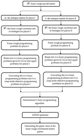
Figure 1.
The flowchart of the proposed algorithm.
Inputs:
- : fuzzy rough payoff matrix
- m: strategies number for player I
- n: strategies number for player II
- : fuzzy rough constraint sets of strategies for player I
- : fuzzy rough constraint sets of strategies for player II
- Step 1. Break down the fuzzy rough programming problem Equation (7) into two programming problems with fuzzy parameters given by the lower problem Equation (9) and the upper problem Equation (10) for player I.
- Step 2. Break down the fuzzy rough programming problem Equation (8) into two programming problems with fuzzy parameters given by the lower problem Equation (11) and the upper problem Equation (12) for player II.
- Step 3. Construct the multi-objective programming problem given in Equation (13) and solve it using Zimmermann’s method [31], hereby obtaining the optimal strategy and the lower bound gain-floor of player I .
- Step 4. Construct the multi-objective programming problem given in Equation (14) and solve it using Zimmermann’s method [31], hereby obtaining the optimal strategy and the upper bound gain-floor of player I .
- Step 5. Construct the multi-objective programming problem given in Equation (15) and solve it using Zimmermann’s method [31], hereby obtaining the optimal strategy and the lower bound loss-ceiling of player II .
- Step 6. Construct the multi-objective programming problem given in Equation (16) and solve it using Zimmermann’s method [31], hereby obtaining the optimal strategy and the upper bound loss-ceiling of player II.
Outputs: The fuzzy rough game value and the optimal strategies for both players.
5. Numerical Example
Now, we illustrate the proposed algorithm by a numerical experiment. Since the constrained matrix game with fuzzy rough payoffs has not been discussed in previous researches, there is no numerical experiment with fuzzy rough payoffs in previous researches. So, we took an example from reference [32] and changed its payoffs to triangular fuzzy rough numbers. Considering:
The coefficient matrices and vectors of the constraint sets of strategies for the player I and II are expressed as follows:
and respectively.
5.1. Computational Results
We obtain the negative and positive ideal solutions of Equation (15) by solving three mathematical programming problems with different objective functions, respectively.
According to Equation (25), the mathematical programming problem is formulated as follows:
Solving Equation (33) using the simplex technique, an optimal solution () can be obtained, where and , and its optimal objective value is represented by
According to Equation (26), the mathematical programming problem can be constructed as follows:
Solving Equation (34) using the simplex technique, an optimal solution () can be obtained, where and , and its optimal objective value is given by
According to Equation (27), the mathematical programming problem can be described as follows:
solving Equation (35) using the simplex technique, an optimal solution () can be obtained, where and , and its optimal objective value is expressed by
Therefore, the positive ideal solution of Equation (15) can be computed as Then, the negative ideal solution of Equation (15) can be written as follows:
and
The relative membership functions of the three objective functions in Equation (15) can be represented as follows:
and
Using Zimmermann’s algorithm [31], Equation (15) is transformed into the linear programming problem as follows:
The optimal solution of Equation (36) can be computed by using the simplex method, where and Then, player II’s lower bound loss-ceiling and optimal strategy are and , respectively.
The same analysis is followed to compute the upper bound game value and optimal strategies of player II and for player I. We obtain the optimal strategies for players I and II as follows:
and the fuzzy rough game value for players I and II are as follows:
Also,
Obviously, the game value for players I and II is the fuzzy rough interval number.
5.2. Discussion
Since the fuzzy rough constrained matrix game has not been discussed in the literature, there are no numerical results in other works for the problem under study. Therefore, the outcomes of our proposed solution are compared to the results obtained from the GAMS software [41]. GAMS is a multi-objective mathematical programming solver that is widely used by many researchers in engineering and economics.
The results obtained by solving the same fuzzy rough constrained matrix game problem using the GAMS software [41] are summarized as follows: player I’s lower bound gain-floor and optimal strategy are and , player I’s upper bound gain-floor and optimal strategy are and . Similarly, player II’s lower bound loss-ceiling and optimal strategy are and and the player II’s upper bound loss-ceiling and optimal strategy are and .
Comparing the results from the GAMS software to the ones from our proposed solution, it is evident that the results are almost the same, which confirms that our proposed approach can solve the fuzzy rough constrained matrix game problem effectively. In addition to that, our approach is applicable to solve many other fuzzy rough matrix games such as fuzzy rough bi-matrix games, fuzzy rough coalition games, and fuzzy rough multi-criteria games.
Analyzing the aforementioned fuzzy multi-objective programming algorithm, we summarize the following advantages of the proposed algorithm:
- Uncertainty is widely common in many real-life models such as roughness, randomness, and fuzziness. Triangular FRNs can appropriately express fuzziness and uncertainty. Our proposed algorithm and models can effectively obtain the optimal strategies of fuzzy rough constrained matrix games.
- Our proposed algorithm is effective in solving fuzzy rough constrained matrix games based on the Zimmermann’s technique [31] and the lower and upper approximation of FRNs, which can decrease the uncertainty to a great extent.
- Our proposed algorithm ensures that any fuzzy rough constrained matrix game has a triangular FRNs-type value, which can be estimated by solving the derived four multi-objective linear programming problems.
6. Conclusions
To the best of the authors’ knowledge, the existing research has not investigated the problem of fuzzy rough constrained matrix games. In this article, we developed an effective fuzzy multi-objective programming algorithm to solve fuzzy rough constrained matrix game. Based on both the upper and lower approximation of the FRNs and the linear programming problems of the classical constrained matrix game, we have constructed new auxiliary fuzzy multi-objective linear programming problems for each player. Furthermore, the proposed approach can ensure that any fuzzy rough constrained matrix game has the fuzzy rough interval-type value, which can be explicitly obtained by solving the derived four multi-objective linear programming problems (i.e., Equations (13–16)). Finally, a numerical experiment of market share game model is given to illustrate the validity of the proposed method.
Our proposed technique is developed to obtain the optimal strategies of constrained matrix games with payoffs of triangular FRNs, which are a special form of FRNs. However, there are many forms of FRNs, such as trapezoidal FRNs, intuitionistic FRNs, convex FRNs, and L-R FRNs. Using these forms of FRNs to describe uncertainty and imprecision in games theory requires further research. Moreover, our proposed method has a wide range of future applications. For example, it can be applied to solve fuzzy rough n-person non-cooperative games, fuzzy rough bi-matrix games, fuzzy rough coalition games, fuzzy rough multi-criteria games, and many other games models.
Author Contributions
All authors contributed equally to the writing of this paper. All authors read and approved the final manuscript.
Funding
This research was funded by the National Key Research Development Program of China (No.2017YFB0305601) and (No. 2017YFB0701700).
Acknowledgments
The authors would like to thank the editor and the anonymous reviewers for their helpful comments for revising the article.
Conflicts of Interest
The authors declare no conflict of interest.
References
- Dubois, D.; Prade, H. Rough Fuzzy Sets and Fuzzy Rough Sets. Int. J. Gen. Syst. 1990, 17, 191–209. [Google Scholar]
- Morsi, N.N.; Yakout, M.M. Axiomatics for Fuzzy Rough Sets. Fuzzy Sets Syst. 1998, 100, 327–342. [Google Scholar] [CrossRef]
- Wang, Y. Mining Stock Price Using Fuzzy Rough Set System. Expert Syst. Appl. 2003, 24, 13–23. [Google Scholar] [CrossRef]
- Shen, Q.; Chouchoulas, A. A Fuzzy-Rough Estimator of Algae Populations. Artif. Intell. Eng. 2001, 15, 13–24. [Google Scholar] [CrossRef]
- Shang, Y. False Positive and False Negative Effects on Network Attacks. J. Stat. Phys. 2018, 170, 141–164. [Google Scholar] [CrossRef]
- Bhatt, R.B.; Gopal, M. On Fuzzy-Rough Sets Approach to Feature Selection. Pattern Recognit. Lett. 2005, 26, 965–975. [Google Scholar] [CrossRef]
- Liu, B. Theory and Practice of Uncertain Programming; Springer: Berlin, Germany, 2009. [Google Scholar]
- Liu, M.; Chen, D.; Wu, C.; Li, H. Fuzzy Reasoning Based on a New Fuzzy Rough Set and Its Application to Scheduling Problems. Comput. Math. Appl. 2006, 51, 1507–1518. [Google Scholar] [CrossRef][Green Version]
- Shang, Y. Robustness of Scale-Free Networks under Attack with Tunable Grey Information. EPL (Europhys. Lett.) 2011, 95, 28005. [Google Scholar] [CrossRef]
- Von Neumann, J.; Morgenstern, D. The Theory of Games in Economic Behavior; Princeton University Press: Princeton, NJ, USA, 1944. [Google Scholar]
- Hung, I.C.; Hsia, K.H.; Chen, L.W. Fuzzy Differential Game of Guarding a Movable Territory. Inf. Sci. 1996, 91, 113–131. [Google Scholar]
- Chun-qiao, T.; Xiao-hong, C. Fuzzy Extension of N-Persons Games Based Choquet Integral. J. Syst. Eng. 2009, 24, 479–483. [Google Scholar]
- Chunqiao, T. Shapley Value For N-Persons Games with Interval Fuzzy Coalition Based on Choquet Extension. J. Syst. Eng. 2010, 25, 451–458. [Google Scholar]
- Xu, J. Zero Sum Two-Person Game with Grey Number Payoff Matrix in Linear Programming. J. Grey Syst. 1998, 10, 225–233. [Google Scholar]
- Ammar, E.-S.; Brikaa, M.G. On Solution of Constraint Matrix Games under Rough Interval Approach. Granul. Comput. 2018, 1–14. [Google Scholar] [CrossRef]
- Bector, C.R.; Chandra, S.; Vijay, V. Matrix Games with Goals and Fuzzy Linear Programming Duality. Fuzzy Optim. Decis. Mak. 2004, 3, 255–269. [Google Scholar] [CrossRef]
- Takahashi, S. The Number of Pure Nash Equilibria in a Random Game with Nondecreasing Best Responses. Games Econ. Behav. 2008, 63, 328–340. [Google Scholar] [CrossRef]
- Tan, C.; Yi, W.; Chen, X. Bertrand Game under a Fuzzy Environment. J. Intell. Fuzzy Syst. 2018, 34, 2611–2624. [Google Scholar] [CrossRef]
- Jana, J.; Roy, S.K. Solution of Matrix Games with Generalised Trapezoidal Fuzzy Payoffs. Fuzzy Inf. Eng. 2018, 10, 213–224. [Google Scholar] [CrossRef]
- Mula, P.; Roy, S.K.; Li, D. Birough Programming Approach for Solving Bi-Matrix Games with Birough Payoff Elements. J. Intell. Fuzzy Syst. 2015, 29, 863–875. [Google Scholar] [CrossRef]
- Li, D.F.; Nan, J.X. An Interval-Valued Programming Approach to Matrix Games with Payoffs of Triangular Intuitionistic Fuzzy Numbers. Iran. J. Fuzzy Syst 2014, 11, 45–57. [Google Scholar]
- Nan, J.-X.; Li, D.-F. Linear Programming Technique for Solving Interval-Valued Constraint Matrix Games. J. Ind. Manag. Optim. 2014, 10, 1059–1070. [Google Scholar] [CrossRef]
- Li, D.; Hong, F. Alfa-Cut Based Linear Programming Methodology for Constrained Matrix Games with Payoffs of Trapezoidal Fuzzy Numbers. Fuzzy Optim. Decis. Mak. 2013, 12, 191–213. [Google Scholar] [CrossRef]
- Roy, S.K. Game Theory Under MCDM and Fuzzy Set Theory Some Problems in Multi-Criteria Decision Making Using Game Theoretic Approach; VDM Verlag Dr. Müller: Salbruken, Germany, 2010. [Google Scholar]
- Jana, J.; Roy, S.K. Dual Hesitant Fuzzy Matrix Games: Based on New Similarity Measure. Soft Comput. 2018, 1–10. [Google Scholar] [CrossRef]
- Aggarwal, A.; Chandra, S.; Mehra, A. Solving Matrix Game with I-Fuzzy Payoffs: Pareto Optimal Security Strategies Approach. Fuzzy Inf. Eng. 2014, 6, 167–192. [Google Scholar] [CrossRef]
- Bhaumik, A.; Roy, S.K.; Deng-Feng, L. Analysis of Triangular Intuitionistic Fuzzy Matrix Games Using Robust Ranking. J. Intell. Fuzzy Syst. 2017, 33, 327–336. [Google Scholar] [CrossRef]
- Roy, S.K.; Bhaumik, A. Intelligent Water Management: A Triangular Type-2 Intuitionistic Fuzzy Matrix Games Approach. Water Resour. Manag. 2018, 32, 949–968. [Google Scholar] [CrossRef]
- Chankong, V.; Haimes, Y.Y. Multiobjective Decision Making: Theory and Methodology; Courier Dover Publications: Mineola, NY, USA, 2008. [Google Scholar]
- Steuer, R.E. Multiple Criteria Optimization: Theory, Computation, and Application; Wiley: Hoboken, NJ, USA, 1986. [Google Scholar]
- Zimmermann, H.J. Fuzzy Set Theory and Its Application; Kluwer Academic Publishers: Boston, MA, USA, 1991. [Google Scholar]
- Li, D.-F. Linear Programming Models and Methods of Matrix Games with Payoffs of Triangular Fuzzy Numbers; Springer Nature: New York, NY, USA, 2016; Volume 328. [Google Scholar]
- Sakawa, M. Fuzzy Sets and Interactive Multiobjective Optimization; Springer Publishing: New York, NY, USA, 1993. [Google Scholar]
- Li, D. Lexicographic Method for Matrix Games with Payoffs of Triangular Fuzzy Numbers. Int. J. Uncertain. Fuzziness Knowl. Based Syst. 2008, 16, 371–389. [Google Scholar] [CrossRef]
- Pawlak, Z. Rough Sets. Int. J. Comput. Inf. Sci. 1982, 11, 341–356. [Google Scholar] [CrossRef]
- Das, A.; Bera, U.K.; Maiti, M. A Profit Maximizing Solid Transportation Model under a Rough Interval Approach. IEEE Trans. Fuzzy Syst. 2017, 25, 485–498. [Google Scholar] [CrossRef]
- Rebolledo, M. Rough Intervals Enhancing Intervals for Qualitative Modeling of Technical Systems. Artif. Intell. 2006, 170, 667–685. [Google Scholar] [CrossRef]
- Xiao, S.; Lai, E.M.K. Rough Programming Approach to Power-Balanced Instruction Scheduling for VLIW Digital Signal Processors. IEEE Trans. Signal. Process. 2008, 56, 1698–1709. [Google Scholar] [CrossRef]
- Ammar, E.; Muamer, M. On Solving Fuzzy Rough Linear Fractional Programming Problem. Int. Res. J. Eng. Technol. 2016, 3, 2099–2120. [Google Scholar]
- Owen, G. Game Theory, 2nd ed.; Academic Press: Cambridge, MA, USA, 1982. [Google Scholar]
- Mavrotas, G. Generation of Efficient Solutions in Multiobjective Mathematical Pro-Gramming Problems Using GAMS. Tech. Rep. 2007, 167–189. [Google Scholar]
© 2019 by the authors. Licensee MDPI, Basel, Switzerland. This article is an open access article distributed under the terms and conditions of the Creative Commons Attribution (CC BY) license (http://creativecommons.org/licenses/by/4.0/).