Solutions of the Nonlinear Integral Equation and Fractional Differential Equation Using the Technique of a Fixed Point with a Numerical Experiment in Extended b-Metric Space

Abstract

The present paper aims to define three new notions: ${\mathsf{\Theta }}_e$-contraction, a Hardy–Rogers-type $\mathsf{\Theta }$-contraction, and an interpolative $\mathsf{\Theta }$-contraction in the framework of extended b-metric space. Further, some fixed point results via these new notions and the study endeavors toward a feasible solution would be suggested for nonlinear Volterra–Fredholm integral equations of certain types, as well as a solution to a nonlinear fractional differential equation of the Caputo type by using the obtained results. It also considers a numerical example to indicate the effectiveness of this new technique.

1. Introduction

The fixed point theory is derived from the investigation of the solution for certain types of differential equations using the successive approximation method. Indeed, the renowned fixed point theorems of Banach [1] are a reformulation of the successive approximation method that was used by some famous mathematicians, namely Cauchy, Liouville, Picard, Lipschitz, Peano, etc. This fact also indicates that the advances and progress in fixed point theory can be referred back to differential equations and the integral equations. On the other hand, in recent years, fixed point theory has been used very extensively to find solutions of nonlinear fractional differential equations.

Indeed, in the last few decades, fractional calculus and fractional differential and integral equations have been the most interesting research topics, not only in mathematics, but also in physics. We can find a brief historical introduction to fractional derivatives with basic notations, illustrations, and results in [2,3,4]. Since the beginning, it has been known that the theory has wide applications not only in nonlinear analysis and computational mathematics, but also in applied sciences, including computer science and economics. The applications of these fixed point theories have been presented in the last century, due to this strong relation of fixed point theory and the applications used in several disciplines.

The authors in [5] proposed the notion of $\mathsf{\Theta }$-contraction as a generalization of a standard contraction, given by Banach, and proved fixed point theorems in the context of Bianciari distance space. We, first, recall the notion of $\mathsf{\Theta }$-contraction, which is based on the following class of auxiliary functions:

$${\displaystyle \mathsf{\Theta }:=\left\{\theta |\theta :(0,\infty )\to (1,\infty )\mathrm{satisfies}\left({\mathsf{\Theta }}_1\right)-\left({\mathsf{\Theta }}_4\right)\right\},}$$

where:

(${\mathsf{\Theta }}_1$)

$\theta$ is non-decreasing;

(${\mathsf{\Theta }}_2$)

for each sequence $\{s_n\}\subset (0,\infty ),{lim}_{n\to \infty }\theta \left(s_n\right)=1\iff {lim}_{n\to \infty }{s}_n=0^{+}$;

(${\mathsf{\Theta }}_3$)

there exist $q\in (0,1)$ and $\ell \in (0,\infty ]$ such that ${lim}_{s\to 0^{+}}\frac{\theta \left(s\right)-1}{s^q}=\ell ;$

(${\mathsf{\Theta }}_4$)

$\theta$ is continuous.

This notion has been used by many authors to provide fixed point results; see, e.g., [6,7,8,9,10,11,12,13,14].

On the other hand, we recall the notion of extended b-metric space (simply, ${\delta }_e$-metric space), introduced by Kamran et al. [15], which is the most general form of the concept of the metric. For the sake of completeness, we recollect the definition as follows:

Definition 1

([15]). For a non-empty set S and a mapping $\omega :S\times S\to [1,\infty )$, we say that a function ${\delta }_e:S\times S\to [0,\infty )$ is called an extended b-metric (in short, ${\delta }_e$-metric) if it satisfies:

(i) 

${\delta }_e(x,y)=0$ if and only if $x=y$;

(ii) 

${\delta }_e(x,y)={\delta }_e(y,x)$;

(iii) 

${\delta }_e(x,y)\le \omega (x,y)[{\delta }_e(x,z)+{\delta }_e(z,y)],$

for all $x,y,z\in S.$ The symbols $(S,{\delta }_e)$ denote ${\delta }_e$-metric space.

Remark 1.

It is clear that in the case of $\theta (x,y)=s$, for $s\ge 1$, the extended b-metric becomes the standard b-metric. As is known well, the b-metric does not need to be continuous. As a result, the extended b-metric is not necessarily continuous either. In this paper, it is presumed that the extended b-metric is continuous.

Example 1.

Let $p\in (0,1)$, $q>1$, and $S=L^p[a,b]\cup L^q[a,b]$ be equipped with the metric:

$${\delta }_e(x,y)=\left\{\begin{array}{cc}\hfill d_p(x,y)& ifx,y\in L^p[a,b],\hfill \\ \hfill d_q(x,y)& ifx,y\in L^q[a,b],\hfill \\ \hfill 0& \mathit{otherwise},\hfill \end{array}\right.$$

where:

$$L_r\left([a,b]\right)=\{x:[a,b]\to \mathbb{R}:{\int }_a^b{\left|x\left(t\right)\right|}^{r}dt<\infty \}forr=p,q.$$

and:

$$d_r(x,y)={\left(\sum _{n=1}^{\infty }{|x_n-y_n|}^r\right)}^{1/r},forr=p,q.$$

It is obvious that $(S,{\delta }_e)$ forms an extended b-metric with:

$$\omega (x,y)=\left\{\begin{array}{cc}\hfill 2^{1/p}& ifx,y\in L^p[a,b]\left(\mathbb{R}\right),\hfill \\ \hfill 2^{1/q}& ifx,y\in L^q[a,b]\left(\mathbb{R}\right),\hfill \\ \hfill 1& \mathit{otherwise}.\hfill \end{array}\right.$$

Example 2.

Let $S=[0,1]$, $\omega :S\times S\to [1,\infty ),\omega (x,y)=\frac{xy+1}{x+y}$, and $\omega (0,0)=\frac{3}{2}$. Define ${\delta }_e:S\times S\to [0,\infty )$ as:

$${\delta }_e(x,y)=\left\{\begin{array}{cc}\hfill \frac{1}{xy},& \mathit{for}x,y\in (0,1],x\ne y\hfill \\ \hfill 0,& \mathit{for}x,y\in [0,1],x=y\hfill \end{array}\right.$$

$${\delta }_e(y,0)={\delta }_e(0,y)=\frac{1}{y},\mathit{for}y\in (0,1].$$

Clearly, (i) and (ii) hold. For (iii), we shall consider the following cases:

Case 1.

Let $x,y\in (0,1],$ for $z\in (0,1]$; we have:

$$\begin{array}{cc}\hfill {\delta }_e(x,& y)\le \omega (x,y)[{\delta }_e(x,z)+{\delta }_e(z,y)]\hfill \\ & \iff \frac{1}{xy}\le \frac{1+xy}{x+y}\left(\frac{1}{xz}+\frac{1}{yz}\right)\hfill \\ & \iff \frac{1}{xy}\le \frac{1+xy}{x+y}\left(\frac{y+x}{xyz}\right)\hfill \\ & \iff z\le 1+xy\hfill \end{array}$$

If $z=0$, then:

$$\begin{array}{cc}\hfill {\delta }_e(x,& y)\le \omega (x,y)[{\delta }_e(x,0)+{\delta }_e(0,y)]\hfill \\ & \iff \frac{1}{xy}\le \omega (x,y)\left(\frac{1}{x}+\frac{1}{y}\right)\hfill \\ & \iff \frac{1}{xy}\le \frac{1+xy}{x+y}\left(\frac{x+y}{xy}\right)\hfill \\ & \iff 1\le 1+xy\hfill \\ & \iff 0\le xy\hfill \end{array}$$

Case 2.

For $x\in (0,1]$ and $y=0,$ let $z\in (0,1]$:

$$\begin{array}{cc}\hfill {\delta }_e(x,& 0)\le \omega (x,0)[{\delta }_e(x,z)+{\delta }_e(z,0)]\hfill \\ & \iff \frac{1}{x}\le \frac{1}{x}\left(\frac{1}{xz}+\frac{1}{z}\right)\hfill \\ & \iff 1\le \frac{1+x}{xz}\hfill \\ & \iff xz\le 1+x\hfill \end{array}$$

Case 3.

For $x=0=y$ and $z\in (0,1]$,

• clearly one can check that ${\delta }_e(x,y)\le \omega (x,y)[{\delta }_e(x,z)+{\delta }_e(z,y)]$.
• Similarly, for $x=0=y$ and $z=0$, the triangle inequality holds.
• Hence, for any $x,y,z\in S,$ ${\delta }_e(x,y)\le \omega (x,y)[{\delta }_e(x,z)+{\delta }_e(z,y)]$.

Definition 2

([15]).Let S be a non-empty set endowed with the extended b-metric ${\delta }_e$, and a sequence $\{x_n\}$ in S is said to:

(a) 

converge to x if for any given $ϵ>0$, there exists $N=N(ϵ)\in \mathbb{N}$ such that ${\delta }_e(x_n,x)<ϵ,$ for all $n\ge N.$ In brief, we write ${\displaystyle \underset{n\to \infty }{lim}{x}_n=x.}$

(b) 

be fundamental (Cauchy) if for every $ϵ>0$, there exists $N=N\left(ϵ\right)\in \mathbb{N}$ such that ${\delta }_e(x_m,x_n)<ϵ,$ for all $m,n\ge N.$

Furthermore, this study defines the completeness of ${\delta }_e$-metric space as follows:

(c) If any fundamental (Cauchy) sequence in S is convergent, then we say that $(S,{\delta }_e)$ is complete.

For more interesting examples and basic results in ${\delta }_e$-metric space, we refer to [16,17,18,19,20]. For some recent modifications or developments to extended $b-$metric spaces, the reader may refer to the so-called controlled and double-controlled metric type spaces in [21,22] and for further fixed point investigations in extended b-metric spaces to [23].

With reference to the above facts, the proposed three new concepts are ${\mathsf{\Theta }}_e$-contraction, a Hardy–Rogers-type $\mathsf{\Theta }$-contraction, and an interpolative $\mathsf{\Theta }$-contraction in ${\delta }_e$-metric space, and we prove pertinent fixed point theorems in Section 2. By using the obtained results in Section 2, we propose the solutions of the nonlinear integral equation and fractional differential equation via the fixed point approach, which are presented in Section 3 and Section 4. The effectiveness of this approach is illustrated by a numerical experiment in Section 5.

2. Main Results

Now, we start this section by introducing the concept of ${\mathsf{\Theta }}_e$-contraction.

Definition 3.

A self-mapping T, on an extended b-metric space $(S,{\delta }_e)$, is named a ${\mathsf{\Theta }}_e$-contraction if there exists a function $\theta \in \mathsf{\Theta }$ such that:

$$\theta \left({\delta }_e(Tx,Ty)\right)\le {\left[\theta \left({\delta }_e(x,y)\right)\right]}^r\mathit{if}{\delta }_e(Tx,Ty)\ne 0\mathit{for}x,y\in S,$$

where $r\in [0,1)$ such that ${\displaystyle \underset{m,n\to \infty }{lim\; sup}\omega (x_n,x_m)<\frac{1}{r};}$ here, $x_n=T^n{x}_0$ for $x_0\in S$.

Theorem 1.

If a self-mapping T, on a completed extended b-metric space $(S,{\delta }_e)$, forms a ${\mathsf{\Theta }}_e$-contraction, then T has a unique fixed point in S.

Proof. For an arbitrary point $x_0\in S$, we construct an iterative sequence ${\{x_n\}}_{0^{\infty }}$ as follows:

$$x_n=T^n{x}_0\mathrm{for}\mathrm{all}n\in \mathbb{N}.$$

Suppose, if $T^{n_{*}}x=T^{n_{*}+1}x$ for some $n_{*}\in \mathbb{N}$, then $T^{n_{*}}x$ will be a fixed point of T.

Therefore, without loss of generality, we can assume that ${\delta }_e(T^{n}x,T^{n+1}x)>0$ for all $n\in \mathbb{N}$. From Definition 3, we have:

$$\begin{array}{cc}\hfill \theta \left({\delta }_e(x_n,x_{n+1})\right)& =\theta \left({\delta }_e(T{x}_{n-1},T{x}_n)\right)\hfill \\ & \le {\left[\theta \left({\delta }_e(x_{n-1},x_n)\right)\right]}^r\hfill \\ & \le {\left[\theta \left({\delta }_e(x_{n-2},x_{n-1})\right)\right]}^{r^2}.\hfill \end{array}$$

Recursively, we find that:

$$\theta \left({\delta }_e(x_n,x_{n+1})\right)\le {\left[\theta \left({\delta }_e(x_0,x_1)\right)\right]}^{r^n}.$$

(1)

Accordingly, we obtain that:

$$1<\theta \left({\delta }_e(x_n,x_{n+1})\right)\le {\left[\theta \left({\delta }_e(x_0,x_1)\right)\right]}^{r^n}\mathrm{for}\mathrm{all}n\in \mathbb{N}.$$

(2)

Letting $n\to \infty$ in (1), we get $\theta \left({\delta }_e(x_n,x_{n+1})\right)\to 1$ as $n\to \infty$.

From $\left({\mathsf{\Theta }}_2\right)$, we have:

$${\displaystyle \underset{n\to \infty }{lim}{\delta }_e(x_n,x_{n+1})=0.}$$

(3)

From $\left({\mathsf{\Theta }}_3\right)$, there exist $q\in (0,1)$ and $\ell \in (0,\infty ]$ such that:

$${\displaystyle \underset{n\to \infty }{lim}{\displaystyle \frac{\theta \left({\delta }_e(x_n,x_{n+1})\right)-1}{{\left[{\delta }_e(x_n,x_{n+1})\right]}^q}}=\ell .}$$

We presume $\ell <\infty$ and $B=\frac{\ell }{2}>0$. On account of the limit definition, there exists $n_0\in \mathbb{N}$ such that:

$$\left|{\displaystyle \frac{\theta \left({\delta }_e(x_n,x_{n+1})\right)-1}{{\left[{\delta }_e(x_n,x_{n+1})\right]}^q}}-\ell \right|\le B$$

for all $n\ge n_0$.

It yields that $\left|{\displaystyle \frac{\theta \left({\delta }_e(x_n,x_{n+1})\right)-1}{{\left[{\delta }_e(x_n,x_{n+1})\right]}^q}}\right|\ge \ell -B=B$ for all $n\ge n_0$.

Then, we derive that:

$$n\left[{\delta }_e{(x_n,x_{n+1})}^q\right]\le n\left[{\displaystyle \frac{\theta \left({\delta }_e(x_n,x_{n+1})\right)-1}{B}}\right]\mathrm{for}\mathrm{all}n\ge n_0.$$

Assume $\ell =\infty$ and $B>0$ (an arbitrary positive number). From the definition of the limit, there exists $n_0\in \mathbb{N}$

such that ${\displaystyle \frac{\theta \left({\delta }_e(x_n,x_{n+1})\right)-1}{{\left[{\delta }_e(x_n,x_{n+1})\right]}^q}}\ge B$ for all $n\ge n_0$.

This implies that:

$$n{\left[{\delta }_e(x_n,x_{n+1})\right]}^q\le n\left[{\displaystyle \frac{\theta \left({\delta }_e(x_n,x_{n+1})\right)-1}{B}}\right]\mathrm{for}\mathrm{all}n\ge n_0.$$

Subsequently, in all cases, there exist $\frac{1}{B}>0$ and $n_0\in \mathbb{N}$ such that:

$$n{\left[{\delta }_e(x_n,x_{n+1})\right]}^q\le n\left[{\displaystyle \frac{\theta \left({\delta }_e(x_n,x_{n+1})\right)-1}{B}}\right]\mathrm{for}\mathrm{all}n\ge n_0.$$

Using Equation (1), we obtain:

$$n{\left[{\delta }_e(x_n,x_{n+1})\right]}^q\le {\left[\theta \left({\delta }_e(x_0,x_1)\right)\right]}^{r^n}-1\mathrm{for}\mathrm{all}n\ge n_0.$$

As $n\to \infty$ in the inequality above, we find:

$${\displaystyle \underset{n\to \infty }{lim}n{\left[{\delta }_e(x_n,x_{n+1})\right]}^q=0.}$$

Thus, there exists $n_1\in \mathbb{N}$ such that:

$${\delta }_e(x_n,x_{n+1})\le {\displaystyle \frac{1}{n^{\frac{1}{q}}}}\mathrm{for}\mathrm{all}n\ge n_1.$$

(4)

Let $N=max\{n_0,n_1\}.$ Due to the modified triangle inequality, we derive that:

$$\begin{array}{cc}\hfill {\delta }_e(x_n,x_{n+m})& =\omega (x_n,x_{n+m})[{\delta }_e(x_n,x_{n+1})+{\delta }_e(x_{n+1},x_{n+m})]\hfill \\ & =\omega (x_n,x_{n+m}){\delta }_e(x_n,x_{n+1})+\omega (x_n,x_{n+m}){\delta }_e(x_{n+1},x_{n+m})\hfill \\ & \le \omega (x_n,x_{n+m}){\delta }_e(x_n,x_{n+1})\hfill \\ & +\omega (x_n,x_{n+m})\omega (x_{n+1},x_{n+m})[{\delta }_e(x_{n+1},x_{n+2})+{\delta }_e(x_{n+2},x_{n+m})]\hfill \\ & \le \omega (x_n,x_{n+m}){\delta }_e(x_n,x_{n+1})+\omega (x_n,x_{n+m})\omega (x_{n+1},x_{n+m}){\delta }_e(x_{n+1},x_{n+2})\hfill \\ & +\omega (x_n,x_{n+m})\omega (x_{n+1},x_{n+m})\omega (x_{n+2},x_{n+m})[{\delta }_e(x_{n+2},x_{n+3})+{\delta }_e(x_{n+3},x_{n+m})]\hfill \\ & ⋮\hfill \\ & \le \omega (x_n,x_{n+m}){\delta }_e(x_n,x_{n+1})+\omega (x_n,x_{n+m})\omega (x_{n+1},x_{n+m}){\delta }_e(x_{n+1},x_{n+2})\hfill \\ & +\cdots +\omega (x_n,x_{n+m})\omega (x_{n+1},x_{n+m})\cdots \omega (x_{n+m-1},x_{n+m}){\delta }_e(x_{n+m-1},x_{n+m})\hfill \end{array}$$

This can be written as,

$${\delta }_e(x_n,x_{n+m})\le \sum _{j=n}^{n+m-1}{\delta }_e(x_j,x_{j+1})\prod _{i=n}^{n+m-1}\omega (x_i,x_{n+m})$$

Since ${\displaystyle \underset{n,m\to \infty }{lim}\omega (x_n,x_m)<\frac{1}{r},}$ we have:

$${\delta }_e(x_n,x_{n+m})\le \sum _{j=n}^{n+m-1}{\delta }_e(x_j,x_{j+1})\prod _{i=n}^{n+m-1}\omega (x_i,x_{n+m})\le \frac{1}{r}\sum _{j=n}^{\infty }{\displaystyle \frac{1}{j^{\frac{1}{q}}}},$$

which is convergent as $n,m\to \infty$ and $\frac{1}{q}>1$.

Thus, the sequence $\left\{x_n\right\}$ in S is a Cauchy sequence. Since $(S,{\delta }_e)$ is a complete ${\delta }_e$-metric space, there exists a point $\eta$ in S such that $\{x_n\}$ converges to $\eta$.

One can easily note that T is continuous. Suppose that $Tx\ne Ty$. Taking the expression (3) into account, we have:

$$\begin{array}{cc}\hfill ln\left[\theta {\delta }_e(Tx,Ty)\right]& \le rln\left[\theta {\delta }_e(x,y)\right]\hfill \\ & \le ln\left[\theta {\delta }_e(x,y)\right].\hfill \end{array}$$

Regarding $\left({\mathsf{\Theta }}_1\right)$, it implies that, ${\delta }_e(Tx,Ty)\le {\delta }_e(x,y)$ for all distinct $x,y\in S$.

From this evaluation, we can get, ${\delta }_e(x_{n+1},T\eta )={\delta }_e(T{x}_n,T\eta )\le {\delta }_e(x_n,\eta )$ for all $n\in \mathbb{N}$.

As $n\to \infty$ in the inequality above, we derive $x_{n+1}\to T\eta$. By the uniqueness of the limit, $T\eta =\eta .$

Suppose f has another fixed point $\zeta$ such that $\eta \ne \zeta$. Then, clearly, ${\delta }_e(\eta ,\zeta )={\delta }_e(f\eta ,f\zeta )\ne 0$.

Now, using the condition (3), we get,

$$\begin{array}{cc}\hfill \theta \left({\delta }_e(\eta ,\zeta )\right)=\theta \left({\delta }_e(T\eta ,T\zeta )\right)& =\theta \left({\delta }_e(T^q\eta ,T^q\zeta )\right)\hfill \\ & \le {\left[\theta \left({\delta }_e(\eta ,\zeta )\right)\right]}^{r^q}\hfill \\ & <\theta \left({\delta }_e(\eta ,\zeta )\right),\mathrm{a}\mathrm{contradiction}.\hfill \end{array}$$

Therefore, $\eta =\zeta$. This claims that T has a unique fixed point in S.  □

Example 3.

Let $S=[0,\infty )$. Define ${\delta }_e:S\times S\to [0,\infty )$ as:

$${\delta }_e(x,y)={(x-y)}^2$$

and $\omega :S\times S\to [1,\infty )$ as $\omega (x,y)=2x+3y+5$. Then, $(S,{\delta }_e)$ is a complete extended b-metric space.

Define $T:X\to X$ as $Tx=\frac{x}{3}$, so that ${\delta }_e(Tx,Ty)={(\frac{x}{3}-\frac{y}{3})}^2\le \frac{1}{8}=r{\delta }_e(x,y)$, where $r=\frac{1}{8}$.

Note that for each $x\in S,$$T^n\left(x\right)=\frac{x}{3^n}$.

We have ${\displaystyle \underset{m,n\to \infty }{lim}\omega (x_m,x_n)=\underset{m,n\to \infty }{lim}2\frac{x}{3^m}+3\frac{x}{3^n}<8=\frac{1}{r}.}$

Now, define $\theta :(0,\infty )\to (1,\infty )$ as $\theta \left(t\right)=e^t$.

Then, all the conditions of Theorem 1 are satisfied so that the mapping $\mathit{T}$ has a unique fixed point “0” in S.

If we take $\omega (x,y)=b>1$ in the above theorem, then we get the below corollary.

Corollary 1.

Let T be a self-mapping on a complete b-metric space $(S,d)$. If there exist $\vartheta \in \mathsf{\Theta }$ and $r\in (0,1)$ such that:

$$\vartheta \left(d(Tx,Ty)\right)\le {\left[\vartheta \left(d(x,y)\right)\right]}^r\mathrm{if}d(Tx,Ty)\ne 0forx,y\in S,$$

then T has a unique fixed point in S.

If we take $\omega (x,y)=1$ in the above theorem, then we get the below corollary.

Corollary 2.

Let T be a self-mapping on a complete metric space $(S,d)$. If there exist $\vartheta \in \mathsf{\Theta }$ and $r\in (0,1)$ such that:

$$\vartheta \left(d(Tx,Ty)\right)\le {\left[\vartheta \left(d(x,y)\right)\right]}^r\mathit{if}d(Tx,Ty)\ne 0forx,y\in S,$$

then T has a unique fixed point in S.

In what follows, we define the second notion, HR-$\mathsf{\Theta }$-contraction, as follows:

Definition 4.

A self-mapping f, on an extended b-metric space $(S,{\delta }_e)$, is called a Hardy–Rogers-type Θ-contraction (HR-Θ-contraction), if there exists a function $\theta \in \mathsf{\Theta }$ and non-negative real number $r<1$ such that:

$$\begin{array}{cc}\hfill \theta \left({\delta }_e(fx,fy)\right)\le & {\left[M_{f,\theta }(x,y)\right]}^r,\hfill \end{array}$$

(5)

for all $x,y\in S$, where:

$$M_{f,\theta }(x,y):=max\{\theta \left({\delta }_e(x,y)\right),\theta \left({\delta }_e(x,fx)\right),\theta \left({\delta }_e(y,fy)\right),\theta \left(\frac{{\delta }_e(x,fy)+{\delta }_e(y,fx)}{2}\right)\}.$$

where ${\displaystyle \underset{n,m\to \infty }{lim\; sup}\omega (x_n,x_m)<\frac{1}{r};}$ here, $x_n=f^n{x}_0$ for $x_0\in S$ and $r\in (0,1).$

Theorem 2.

If a self-mapping T, on a completed extended b-metric space $(S,{\delta }_e)$ forms an HR-Θ-contraction, then T has a unique fixed point in S.

Proof. 

As in Theorem 1, we construct an iterative sequence ${\{x_n\}}_{0^{\infty }}$ by starting at an arbitrary point $x_0\in S$ as follows:

$$x_n=f^n{x}_0\mathrm{for}\mathrm{all}n\in \mathbb{N}.$$

Without loss of generality, we suppose that ${\delta }_e(f^{n}x,f^{n+1}x)>0$ for all $n\in \mathbb{N}$. Indeed, if $f^{n_{*}}x=f^{n_{*}+1}x$ for some $n_{*}\in \mathbb{N}$, then $f^{n_{*}}x$ will be a fixed point of T.

We prove that ${\displaystyle \underset{n\to \infty }{lim}{\delta }_e(x_n,x_{n+1})=0}$.

Employing the contraction condition (5), we get,

$$\theta \left({\delta }_e(x_{n+1},x_n)\right)\le {\left[M_{f,\theta }(x_n,x_{n-1})\right]}^r,$$

(6)

where:

$$\begin{array}{cc}\hfill M_{f,\theta }(x_n,x_{n-1})& =max\{\theta \left({\delta }_e(x_n,x_{n-1})\right),\theta \left({\delta }_e(x_n,f{x}_n)\right),\theta \left({\delta }_e(x_{n-1},f{x}_{n-1})\right),\hfill \\ & \theta \left(\frac{{\delta }_e(x_n,f{x}_{n-1})+{\delta }_e(x_{n-1},f{x}_n)}{2}\right)\}\hfill \\ & =max\{\theta \left({\delta }_e(x_n,x_{n-1})\right),\theta \left({\delta }_e(x_n,x_{n+1})\right),\theta \left({\delta }_e(x_{n-1},x_n)\right),\hfill \\ & \theta \left(\frac{{\delta }_e(x_{n-1},x_n)+{\delta }_e(x_n,x_{n+1})}{2}\right)\}.\hfill \\ & \le max\{\theta \left({\delta }_e(x_n,x_{n-1})\right),\theta \left({\delta }_e(x_n,x_{n+1})\right)\}.\hfill \end{array}$$

If $M_{f,\theta }(x_n,x_{n-1})=\theta \left({\delta }_e(x_n,x_{n+1})\right)$, then the inequality (6) becomes:

$$\theta \left({\delta }_e(x_{n+1},x_n)\right)\le \theta {\left({\delta }_e(x_n,x_{n+1})\right)}^r\iff ln\left(\theta \left({\delta }_e(x_{n+1},x_n)\right)\right)\le rln\left(\theta \left({\delta }_e(x_{n+1},x_n)\right)\right),$$

which is a contradiction (since $r<1$). Thus, we have $M_{f,\theta }(x_n,x_{n-1})=\theta \left({\delta }_e(x_{n_1},x_n)\right)$. It is yielded from (6) that:

$$\theta \left({\delta }_e(x_n,x_{n+1})\right)\le {\left[\theta \left({\delta }_e(x_n,x_{n-1})\right)\right]}^r.$$

Iteratively, we find that:

$$\theta \left({\delta }_e(x_n,x_{n+1})\right)\le {\left[\theta \left({\delta }_e(x_0,x_1)\right)\right]}^{r^n}.$$

After this observation, by following the related lines in the proof of Theorem 2, we conclude that the sequence $\{x_n\}$ in S is a Cauchy sequence. Regarding that $(S,{\delta }_e)$ is a complete ${\delta }_e$-metric space, there exists a point $\eta$ in S such that $\{x_n\}$ converges to $\eta$.

Without lose of generality, we may assume that $f^{n}x\ne \eta$ for all n (or, for large enough n.) Assume that ${\delta }_e(\eta ,T\eta )>0.$ Employing (5), we get:

$$\theta \left({\delta }_e(f{x}_n,f\eta )\right)\le {\left[M_{f,\theta }(x_n,\eta )\right]}^r,$$

for all $x,y\in S$, where:

$$M_{f,\theta }(x_n,\eta ):=max\{\theta \left({\delta }_e(x_n,\eta )\right),\theta \left({\delta }_e(x_n,f{x}_n)\right),\theta \left({\delta }_e(\eta ,f\eta )\right),\theta \left(\frac{{\delta }_e(x_n,f\eta )+{\delta }_e(\eta ,f{x}_n)}{2}\right)\}.$$

By taking $n\to \infty$ in the inequality above, we derive that:

$$\theta \left({\delta }_e(\eta ,f\eta )\right)\le {\left[\theta \left({\delta }_e(\eta ,f\eta )\right)\right]}^r<\theta \left({\delta }_e(\eta ,f\eta )\right),$$

a contradiction. Hence, $f\eta =\eta .$

That is, f has a fixed point in S.

Suppose f has another fixed point $\zeta$ such that $\eta \ne \zeta$.

Then, clearly, ${\delta }_e(\eta ,\zeta )={\delta }_e(f\eta ,f\zeta )\ne 0$.

Now, using the condition (7), we get,

$$\begin{array}{cc}\hfill 1<\theta \left({\delta }_e(\eta ,\zeta )\right)& =\theta \left({\delta }_e(f\eta ,f\zeta )\right)\hfill \\ & \le [max\{\theta \left({\delta }_e(\eta ,\zeta )\right),\theta \left({\delta }_e(\eta ,f\eta )\right),\theta \left({\delta }_e(\zeta ,f\zeta )\right),\hfill \\ & \theta ({\delta }_e(\eta ,f\zeta )+{\delta }_e(\zeta ,f\eta )){\left\}\right]}^r\hfill \\ & <\theta \left({\delta }_e(\eta ,\zeta )\right),\hfill \end{array}$$

a contradiction. Accordingly, we have $\eta =\zeta$.

Thus, f has a unique fixed point in S.  □

Definition 5.

Let $(S,{\delta }_e)$ be a ${\delta }_e$-metric space and $f:X\to X$ be a mapping. Then, f is said to be an interpolative-Θ-contraction if there exists a function $\theta \in \mathsf{\Theta }$ and non-negative real numbers $r_1,r_2,r_3,r_4$ with $r_1+r_2+r_3+2r_4<1$ such that:

$$\begin{array}{cc}\hfill \theta \left({\delta }_e(fx,fy)\right)\le & {\left[\theta \left({\delta }_e(x,y)\right)\right]}^{r_1}{\left[\theta \left({\delta }_e(x,fx)\right)\right]}^{r_2}\hfill \\ & {\left[\theta \left({\delta }_e(y,fy)\right)\right]}^{r_3}{\left[\theta ({\delta }_e(x,fy)+{\delta }_e(y,fx))\right]}^{r_4},\hfill \end{array}$$

(7)

for all $x,y\in S$.

Where ${\displaystyle \underset{n,m\to \infty }{lim\; sup}\omega (x_n,x_m)<\frac{1}{r};}$ here, $x_n=f^n{x}_0$ for $x_0\in S$ and $r\in (0,1).$

Theorem 3.

Let $(S,{\delta }_e)$ be a complete ${\delta }_e$-metric space such that ${\delta }_e$ is a continuous functional and $f:X\to X$ be an interpolative-Θ-contraction. Then, f has a unique fixed point in S.

We skip the proof since:

$$\begin{array}{c}{\left[\theta \left({\delta }_e(x,y)\right)\right]}^{r_1}{\left[\theta \left({\delta }_e(x,fx)\right)\right]}^{r_2}{\left[\theta \left({\delta }_e(y,fy)\right)\right]}^{r_3}{\left[\theta ({\delta }_e(x,fy)+{\delta }_e(y,fx))\right]}^{r_4}\\ \le {\left[M_{\theta ,f}(x,y)\right]}^{r_1+r_2+r_3+2r_4}.\end{array}$$

Thus, it is sufficient to choose $r:=r_1+r_2+r_3+2r_4<1$ in Theorem 2 to conclude the theorem above.

In Theorem 3, if we take $r_2=0,r_3=0,r_4=0$, then the above theorem reduces to as below.

Corollary 3.

labelJS1-c-4 Let $(S,{\delta }_e)$ be an extended b-metric space and $\theta \in \mathsf{\Theta }$. If a mapping $f:X\to X$ satisfies that

there exists $r_1\in [0,1)$ such that:

$$\theta \left({\delta }_e(fx,fy)\right)\le {\left[\theta \left({\delta }_e(x,y)\right)\right]}^{r_1}\mathit{for}\mathit{all}x,y\in S$$

(8)

where $r\in [0,1)$ and ${\displaystyle \underset{m,n\to \infty }{lim\; sup}\omega (x_n,x_m)<\frac{1}{r}}$, then f has a unique fixed point in S.

In Theorem 3, if we take $r_1=0,r_2=0,r_3=0$, then the above theorem reduces to as below.

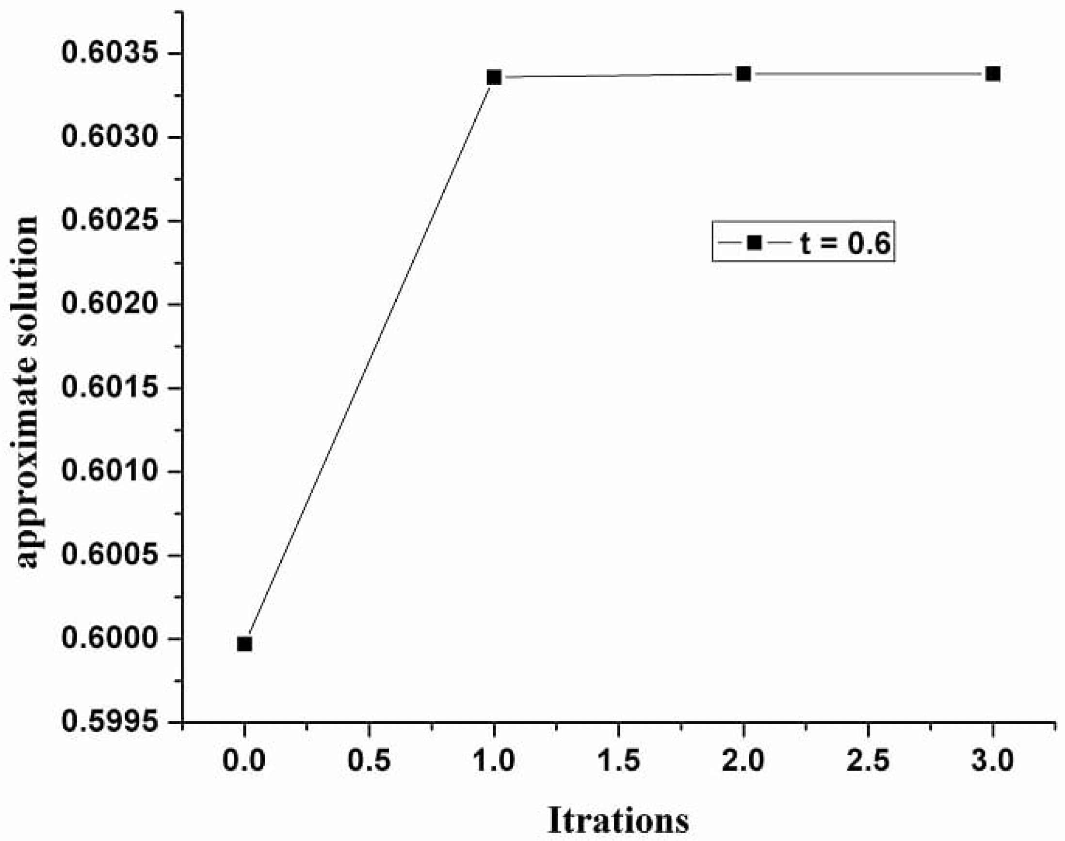
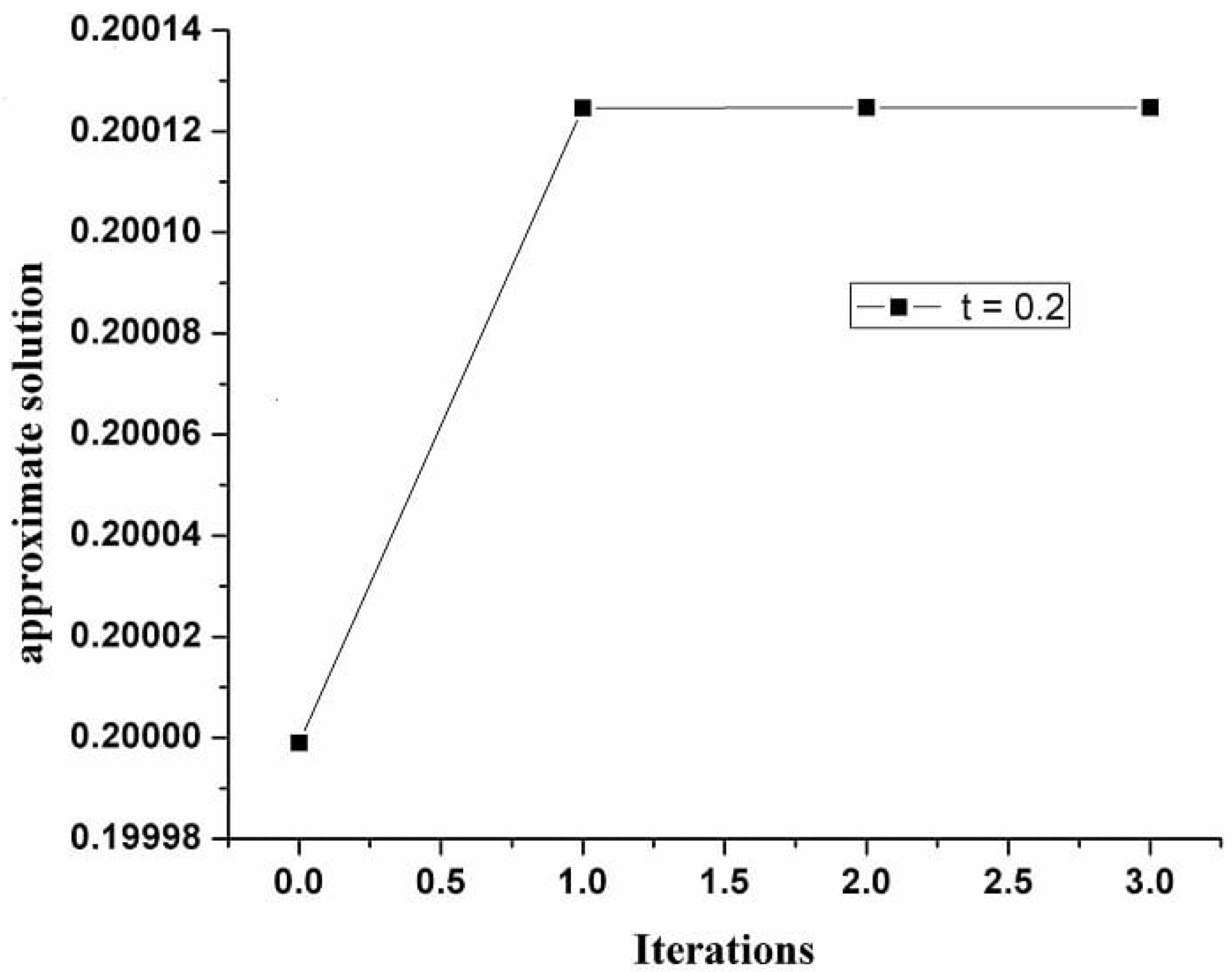
Corollary 4.

labelJS1-c-4 Let $(S,{\delta }_e)$ be an extended b-metric space such that ${\delta }_e$ is a continuous functional, $\theta \in \mathsf{\Theta }$, and $f:X\to X$ be a mapping. Suppose that there exists $r_4\in [0,1)$ such that:

$$\theta \left({\delta }_e(fx,fy)\right)\le {\left[\theta ({\delta }_e(x,fy)+{\delta }_e(y,fx))\right]}^{r_4}\mathit{for}\mathit{all}x,y\in S$$

(9)

and $r\in [0,1)$ such that ${\displaystyle \underset{m,n\to \infty }{lim\; sup}\omega (x_n,x_m)<\frac{1}{r}}$. Then, f has a unique fixed point in S.

3. Fixed Point Method for the Common Solution of Nonlinear Volterra–Fredholm Integral Equations

Let $X:=C([a,b],\mathbb{R})$; the set of all continuous real valued functions is defined on $[a,b]$. Define ${\delta }_e:S\times S\to \mathbb{R}$ and $\gamma :S\times S\to [1,\infty )$ by:

$${\delta }_e(x,y)={sup|x\left(t\right)+y\left(t\right)|}^2,t\in [a,b]\mathrm{and}\gamma (x,y)=\left|x\left(t\right)\right|+\left|y\left(t\right)\right|+1.$$

Clearly, $(S,{\delta }_e)$ is a complete extended b-metric space.

Consider the nonlinear Volterra–Fredholm integral equation:

$$x\left(t\right)={\lambda }_1{\int }_a^t{\kappa }_1(t,s,x\left(s\right))ds+{\lambda }_2{\int }_a^b{\kappa }_2(t,s,x\left(s\right))ds;a\le t\le b,$$

(10)

where $x\left(t\right)$ is the unknown solution, ${\kappa }_i(t,s,x\left(s\right));(i=1,2)$ are called smooth functions, and ${\lambda }_i,$a, and b are constants.

Let us assume $a=0$ for an effortlessness detailed examination of the nonlinear Volterra–Fredholm integral Equation (10).

Suppose that the following conditions hold:

• the mapping $f:C[0,b]\to C[0,b]$ defined by:

  $$f\left(x\left(t\right)\right)={\lambda }_1{\int }_0^t{\kappa }_1(t,s,x\left(s\right))ds+{\lambda }_2{\int }_0^b{\kappa }_2(t,s,x\left(s\right))ds;$$
  $\mathrm{for}\mathrm{all}x\in C[0,b]\mathrm{and}0\le s\le t\le b,$ is a continuous mapping and
  ${\kappa }_i:[0,b]\times [0,b]\times \mathbb{R}\to \mathbb{R}$
• $\mathsf{{\rm Y}}:[0,\infty )\to [1,\infty )$ with $\mathsf{{\rm Y}}\left(t\right)<t$ for all $t>0.$
• ${\kappa }_i$ for some constant ${\mathcal{A}}_i$ satisfies:

  $$|{\kappa }_i(t,s,x\left(s\right))-{\kappa }_i(t,s,y\left(s\right))|\le {\mathcal{A}}_i\left[\mathsf{{\rm Y}}\right(|x\left(s\right)-{y\left(s\right)\left|\right)]}^{\frac{r_1}{2}},$$

  where $0\le s\le t\le b,i=1,2.$
• Further suppose that $\varrho t+\eta b<1,$ where $\varrho ={\lambda }_1{\mathcal{A}}_1$ and $\eta ={\lambda }_2{\mathcal{A}}_2$.

Then, the nonlinear Volterra–Fredholm Equation (10) has a unique solution.

Consider:

$$\begin{array}{cc}\hfill {|fx\left(t\right)-fy\left(t\right)|}^2& =|{\lambda }_1{\int }_0^t{\kappa }_1(t,s,x\left(s\right))ds+{\lambda }_2{\int }_0^b{\kappa }_2(t,s,x\left(s\right))ds\hfill \\ & -\left({\lambda }_1{\int }_0^t{\kappa }_1(t,s,y\left(s\right))ds+{\lambda }_2{\int }_0^b{\kappa }_2(t,s,y\left(s\right))ds\right){|}^2\hfill \\ & =|{\lambda }_1\left[{\int }_0^t({\kappa }_1(t,s,x\left(s\right))-{\kappa }_1(t,s,y\left(s\right)))ds\right]\hfill \\ & +{\lambda }_2\left[{\int }_0^b({\kappa }_2(t,s,x\left(s\right))-{\kappa }_2(t,s,y\left(s\right)))ds\right]{|}^2\hfill \\ & \le |{\lambda }_1{\mathcal{A}}_1\left(\mathsf{{\rm Y}}\right|x\left(s\right)-{y\left(s\right)\left|\right)}^{\frac{r_1}{2}}t+{\lambda }_2{\mathcal{A}}_2\left(\mathsf{{\rm Y}}\right|x\left(s\right)-{y\left(s\right)\left|\right)}^{\frac{r_1}{2}}b{|}^2\hfill \\ & =\left|(\varrho t+\eta )\right(\mathsf{{\rm Y}}|x\left(s\right)-{y\left(s\right)\left|\right)}^{\frac{r_1}{2}}{|}^2\hfill \\ & <{\left(\mathsf{{\rm Y}}\left(\right|x\left(s\right)-y\left(s\right)|\right)}^{r_1}\hfill \\ & ={\left(\mathsf{{\rm Y}}({\delta }_e(x,y)\right)}^{r_1}\hfill \end{array}$$

This gives,

$$\underset{t\in [0,b]}{sup}{|fU\left(t\right)-fV\left(t\right)|}^2\le {\left(\mathsf{{\rm Y}}{\delta }_e(x\left(t\right),y\left(t\right))\right)}^{r_1},$$

which implies,

$${\delta }_e(f\left(x\left(t\right)\right),f\left(y\left(t\right)\right))\le {\left(\mathsf{{\rm Y}}{\delta }_e(x\left(t\right),y\left(t\right))\right)}^{r_1},\mathrm{for}\mathrm{all}x,y\in S.$$

which yields,

$$\begin{array}{cc}\hfill \mathsf{{\rm Y}}\left({\delta }_e(f\left(x\left(t\right)\right),f\left(y\left(t\right)\right))\right)& \le {\delta }_e(f\left(x\left(t\right)\right),f\left(y\left(t\right)\right))\hfill \\ & \le {\left(\mathsf{{\rm Y}}{\delta }_e(x\left(t\right),y\left(t\right))\right)}^{r_1}\hfill \end{array}$$

It follows that f satisfies all the conditions of Corollary 1. Hence, f has a unique fixed point. This yields that there exists a unique solution of the non-linear Volterra–Fredholm integral equation.

4. Fixed Point Method for Common Solution of Nonlinear Fractional Differential Equations

In this section, by using Corollary 2, we investigate the existence and uniqueness solution for nonlinear fractional differential equations (NFDE), in the sense of the Caputo derivative. Recall that the Caputo fractional derivative of $\wp \left(t\right)$ order $\varrho >0$ is denoted by ${}^{\mathcal{C}}{\mathcal{D}}^{\varrho }\wp \left(t\right)$, and it is defined as:

$${}^{\mathcal{C}}{\mathcal{D}}^{\varrho }\wp \left(t\right)=\frac{1}{\mathsf{\Gamma }(n-\varrho )}{\int }_0^t{(t-\tau )}^{n-\varrho -1}{\wp }^n\left(\tau \right)d\tau ;$$

with $n=[\varrho ]+1\in \mathbb{N},$ where $\varrho \in [n-1,n)$ and $[\varrho ]$ denotes the greatest integer of $\varrho$ (i.e., the integral part of $\varrho$) and $\wp :[0,\infty )\to \mathbb{R}$ is a continuous function.

Here, $S=C([0,1],\mathbb{R})$ denotes the set of all continuous functions from $[0,1]$ into $\mathbb{R}$.

In this section, we shall investigate the existence of uniqueness solutions to a non-linear fractional differential equation.

$${}^{\mathcal{C}}{\mathcal{D}}^{\varrho }\left(x\left(t\right)\right)=h(t,x\left(t\right))$$

(11)

with the integral boundary conditions $x\left(0\right)=0,x\left(1\right)={\int }_0^{\rho }x\left(\tau \right)d\tau ;$ where $x\in S,t,\rho \in (0,1),\varrho \in (1,2]$ and $h:[0,1]\times \mathbb{R}\to \mathbb{R}$ is a continuous function.

Recall that $x\in S$ forms a solution for (11) whenever $x\in S$ forms a solution for the following fractional integral equation:

$$\begin{array}{cc}\hfill x\left(t\right)=& \frac{1}{\mathsf{\Gamma }\left(\varrho \right)}{\int }_0^t{(t-\tau )}^{\varrho -1}h(\tau ,x\left(\tau \right))d\tau \hfill \\ & -\frac{2t}{(2-{\rho }^2)\mathsf{\Gamma }\left(\varrho \right)}{\int }_0^1{(1-\tau )}^{\varrho -1}h(\tau ,x\left(\tau \right))d\tau \hfill \\ & +\frac{2t}{(2-{\rho }^2)\mathsf{\Gamma }\left(\varrho \right)}{\int }_0^{\rho }\left({\int }_0^{\tau }{(\tau -\vartheta )}^{\varrho -1}h(\vartheta ,x\left(\vartheta \right))d\vartheta \right)d\tau .\hfill \end{array}$$

Define the operator $\mathsf{{\rm Y}}:X\to X$ by:

$$\begin{array}{cc}\hfill \mathsf{{\rm Y}}x\left(t\right)=& \frac{1}{\mathsf{\Gamma }\left(\varrho \right)}{\int }_0^t{(t-\tau )}^{\varrho -1}h(\tau ,x\left(\tau \right))d\tau \hfill \\ & -\frac{2t}{(2-{\rho }^2)\mathsf{\Gamma }\left(\varrho \right)}{\int }_0^1{(1-\tau )}^{\varrho -1}h(\tau ,x\left(\tau \right))d\tau \hfill \\ & +\frac{2t}{(2-{\rho }^2)\mathsf{\Gamma }\left(\varrho \right)}{\int }_0^{\rho }\left({\int }_0^{\tau }{(\tau -\vartheta )}^{\varrho -1}h(\vartheta ,x\left(\vartheta \right))d\vartheta \right)d\tau .\hfill \end{array}$$

where S forms a ${\delta }_e$-metric space with:

$${\delta }_e(x,y)=\underset{t\in [0,1]}{sup}{|x\left(t\right)-y\left(t\right)|}^q,\mathrm{for}\mathrm{all}x,y\in S,\mathrm{with}\mathrm{coefficient}s=2^{q-1}.$$

Now, we will prove that the NFDE (11) has a unique solution if the following assumption holds:

$$|h(b,{\eta }_1)-h(b,{\eta }_2)|\le \mathsf{\Gamma }(\varrho +1){\left(\theta {\left(|{\eta }_1-\mathsf{{\rm Y}}{\eta }_2{|}^q+{|{\eta }_2-\mathsf{{\rm Y}}{\eta }_1|}^q\right)}^q\right)}^{\frac{r_4}{q}}$$

where $q>1$ and $\theta :[0,\infty )\to [1,\infty )$ with $\theta \left(t\right)<t$ for all $t>0.$ We need to prove that the condition (9) of Corollary 2 holds. Consider,

$$\begin{array}{cc}\hfill \left|\mathsf{{\rm Y}}x\right(t)-\mathsf{{\rm Y}}y(t\left)\right|=& |\frac{1}{\mathsf{\Gamma }\left(\varrho \right)}{\int }_0^t{(t-\tau )}^{\varrho -1}h(\tau ,x\left(\tau \right))d\tau \hfill \\ & -\frac{2t}{(2-{\rho }^2)\mathsf{\Gamma }\left(\varrho \right)}{\int }_0^1{(1-\tau )}^{\varrho -1}h(\tau ,x\left(\tau \right))d\tau \hfill \\ & +\frac{2t}{(2-{\rho }^2)\mathsf{\Gamma }\left(\varrho \right)}{\int }_0^{\rho }\left({\int }_0^{\tau }{(\tau -\vartheta )}^{\varrho -1}h(\vartheta ,x\left(\vartheta \right))d\vartheta \right)d\tau \hfill \\ & -\frac{1}{\mathsf{\Gamma }\left(\varrho \right)}{\int }_0^t{(t-\tau )}^{\varrho -1}h(\tau ,y\left(\tau \right))d\tau \hfill \\ & +\frac{2t}{(2-{\rho }^2)\mathsf{\Gamma }\left(\varrho \right)}{\int }_0^1{(1-\tau )}^{\varrho -1}h(\tau ,y\left(\tau \right))d\tau \hfill \\ & -\frac{2t}{(2-{\rho }^2)\mathsf{\Gamma }\left(\varrho \right)}{\int }_0^{\rho }\left({\int }_0^{\tau }{(\tau -\vartheta )}^{\varrho -1}h(\vartheta ,y\left(\vartheta \right))d\vartheta \right)d\tau |\hfill \\ & \le \frac{1}{\mathsf{\Gamma }\left(\varrho \right)}{\int }_0^t{(t-\tau )}^{\varrho -1}|h(\tau ,x\left(\tau \right))-h(\tau ,y\left(\tau \right))|d\tau \hfill \\ & +\frac{2t}{(2-{\rho }^2)\mathsf{\Gamma }\left(\varrho \right)}{\int }_0^1{(1-\tau )}^{\varrho -1}|h(\tau ,x\left(\tau \right))-h(\tau ,y\left(\tau \right))|d\tau \hfill \\ & +\frac{2t}{(2-{\rho }^2)\mathsf{\Gamma }\left(\varrho \right)}{\int }_0^{\rho }\left|{\int }_0^{\tau }{(\tau -\vartheta )}^{\varrho -1}[h(\vartheta ,x\left(\vartheta \right))-h(\vartheta ,y\left(\vartheta \right))]d\vartheta \right|d\tau \hfill \\ & \le \frac{1}{\mathsf{\Gamma }\left(\varrho \right)}{\int }_0^t{(t-\tau )}^{\varrho -1}\mathsf{\Gamma }(\varrho +1){\left(\theta \left[\right|x\left(\tau \right)-\mathsf{{\rm Y}}y\left(\tau \right){|}^q+|y\left(\tau \right)-\mathsf{{\rm Y}}x\left(\tau \right){|}^q]\right)}^{\frac{r_4}{4}}d\tau \hfill \\ & +\frac{2t}{(2-{\rho }^2)\mathsf{\Gamma }\left(\varrho \right)}{\int }_0^1{(1-\tau )}^{\varrho -1}\mathsf{\Gamma }(\varrho +1){\left(\theta \left[\right|x\left(\tau \right)-\mathsf{{\rm Y}}y\left(\tau \right){|}^q+|y\left(\tau \right)-\mathsf{{\rm Y}}x\left(\tau \right){|}^q]\right)}^{\frac{r_4}{4}}d\tau \hfill \\ & +\frac{2t}{(2-{\rho }^2)\mathsf{\Gamma }\left(\varrho \right)}{\int }_0^{\rho }{\int }_0^{\tau }{(\tau -\vartheta )}^{\varrho -1}\mathsf{\Gamma }(\varrho +1){\left(\theta \left[\right|x\left(\tau \right)-\mathsf{{\rm Y}}y\left(\tau \right){|}^q+|y\left(\tau \right)-\mathsf{{\rm Y}}x\left(\tau \right){|}^q]\right)}^{\frac{r_4}{4}}d\tau \hfill \\ & \le \mathsf{\Gamma }(\varrho +1){\left(\theta \left[\right|x\left(\tau \right)-\mathsf{{\rm Y}}y\left(\tau \right){|}^q+|y\left(\tau \right)-\mathsf{{\rm Y}}x\left(\tau \right){|}^q]\right)}^{\frac{r_4}{q}}\hfill \\ & \frac{1}{\mathsf{\Gamma }\left(\varrho \right)}({\int }_0^t{(t-\tau )}^{\varrho -1}d\tau +\frac{2t}{(2-{\rho }^2)}{\int }_0^1{(1-\tau )}^{\varrho -1}d\tau \hfill \\ & +\frac{2t}{(2-{\rho }^2)}{\int }_0^{\rho }{\int }_0^{\tau }{(\tau -\vartheta )}^{\varrho -1}d\vartheta d\tau )\hfill \\ & \le \mathsf{\Gamma }(\varrho +1){\left(\theta ({\delta }_e(x,\mathsf{{\rm Y}}y)+{\delta }_e(y,\mathsf{{\rm Y}}x))\right)}^{\frac{r_4}{q}}\hfill \\ & \frac{1}{\mathsf{\Gamma }\left(\varrho \right)}\left(\frac{t^{\varrho }}{\varrho }+\frac{2t}{(2-{\rho }^2)}\frac{1}{\varrho }+\frac{2t}{(2-{\rho }^2)}\frac{{\rho }^{\varrho +1}}{\varrho (\varrho +1)}\right)\hfill \\ & \le \mathsf{\Gamma }(\varrho +1){\left(\theta ({\delta }_e(x,\mathsf{{\rm Y}}y)+{\delta }_e(y,\mathsf{{\rm Y}}x))\right)}^{\frac{r_4}{q}}\hfill \\ & \frac{1}{\mathsf{\Gamma }(\varrho +1)}\underset{t\in (0,1)}{sup}\left(t^{\varrho }+\frac{2t}{(2-{\rho }^2)}+\frac{2t}{(2-{\rho }^2)}\frac{{\rho }^{\varrho +1}}{(\varrho +1)}\right)\hfill \\ & \le {\left(\theta ({\delta }_e(x,\mathsf{{\rm Y}}y)+{\delta }_e(y,\mathsf{{\rm Y}}x))\right)}^{\frac{r_4}{q}}\hfill \end{array}$$

Thus, for $q>1$, we can write:

$${|\mathsf{{\rm Y}}x\left(t\right)-\mathsf{{\rm Y}}y\left(t\right)|}^q\le {\left(\theta ({\delta }_e(x\left(t\right),\mathsf{{\rm Y}}y\left(t\right))+{\delta }_e(y\left(t\right),\mathsf{{\rm Y}}x\left(t\right)))\right)}^{r_4}.$$

Therefore,

$$\underset{t\in [0,1]}{sup}{|\mathsf{{\rm Y}}x\left(t\right)-\mathsf{{\rm Y}}y\left(t\right)|}^q\le {\left(\theta ({\delta }_e(x\left(t\right),\mathsf{{\rm Y}}y\left(t\right))+{\delta }_e(y\left(t\right),\mathsf{{\rm Y}}x\left(t\right)))\right)}^{r_4}$$

$$\Rightarrow {\delta }_e(\mathsf{{\rm Y}}x\left(t\right),\mathsf{{\rm Y}}y\left(t\right))\le {\left(\theta ({\delta }_e(x\left(t\right),\mathsf{{\rm Y}}y\left(t\right))+{\delta }_e(y\left(t\right),\mathsf{{\rm Y}}x\left(t\right)))\right)}^{r_4}$$

This implies,

$$\begin{array}{cc}\hfill \theta \left({\delta }_e(\mathsf{{\rm Y}}x\left(t\right),\mathsf{{\rm Y}}y\left(t\right))\right)& \le {\delta }_e(\mathsf{{\rm Y}}x\left(t\right),\mathsf{{\rm Y}}y\left(t\right))\hfill \\ & \le {\left(\theta ({\delta }_e(x\left(t\right),\mathsf{{\rm Y}}y\left(t\right))+{\delta }_e(y\left(t\right),\mathsf{{\rm Y}}x\left(t\right)))\right)}^{r_4}\hfill \end{array}$$

As a result, this study concludes that all axioms of the Corollary 2 are fulfilled. Hence, $\mathsf{{\rm Y}}$ has a unique fixed point, and the mentioned NFDE has a unique solution.

5. Numerical Example

In this section, a numerical example is established to indicate the significance of the given results.

Let S be a set of all continuous real-valued functions defined on [0,1], i.e., $S=C([0,1],\mathbb{R})$. Define ${\delta }_e:S\times S\to \mathbb{R}$ and $\omega :S\times S\to [1,\infty )$ by ${\delta }_e(x,y)={sup}_{t\in [0,1]}{|x\left(t\right)-y\left(t\right)|}^2$ and $\omega (x,y)=3\left|x\right(t\left)\right|+5\left|y\right(t\left)\right|+2$, respectively. Clearly, $(S,{\delta }_e)$ is a complete ${\delta }_e$-metric space.

Let $f:X\to X$ be the operator defined by:

$$fx\left(t\right)=\vartheta \left(t\right)+{\int }_0^1\kappa (t,s)x\left(s\right)ds;x\left(t\right)\in S.$$

(12)

Let $\vartheta \left(t\right)=tcos\left(t\right),\kappa (t,s)=t$, and $x\left(s\right)=sin\left(x\right(s\left)\right)$. Then, (5.1) becomes:

$$fx\left(t\right)=tcos\left(t\right)+{\int }_0^{1}tsin\left(x\left(s\right)\right)ds;x\left(t\right)\in S.$$

(13)

Suppose the following conditions hold.

• $\vartheta \left(t\right),\kappa (t,s)$, and $x\left(s\right)$ are continuous
• $\mathsf{{\rm Y}}:[0,\infty )\to [1,\infty )$ with $\mathsf{{\rm Y}}\left(t\right)<t$ for all $t>0$
• $|sin\left(x\left(s\right)\right)-sin\left(y\left(s\right)\right)|\le {\left(\mathsf{{\rm Y}}\right|x\left(s\right)-y\left(s\right)|}^2{)}^{\frac{r_1}{2}}$

Consider,

$$\begin{array}{cc}\hfill {|fx\left(t\right)-fy\left(t\right)|}^2& =|tcos\left(t\right)+{\int }_0^{1}tsin\left(x\left(t\right)\right)ds-tcos\left(t\right)+{\int }_0^1{tsin\left(y\left(t\right)\right)ds|}^2\hfill \\ & =|{\int }_0^{1}tsin\left(x\left(t\right)\right)ds-{\int }_0^1{tsin\left(y\left(t\right)\right)ds|}^2\hfill \\ & =|{\int }_0^1{t[sin\left(x\left(t\right)\right)-sin\left(y\left(t\right)\right)]ds|}^2\hfill \\ & ={\int }_0^1{\left|t\right|}^2{|sin\left(x\left(t\right)\right)-sin\left(y\left(t\right)\right)|}^{2}ds\hfill \\ & <{\left[{\left(\mathsf{{\rm Y}}\right|x\left(s\right)-y\left(s\right)|}^2{)}^{\frac{r_1}{2}}\right]}^2{\int }_0^{1}ds\hfill \\ & ={\left(\mathsf{{\rm Y}}\right|x\left(s\right)-y\left(s\right)|}^2{)}^{r_1}\hfill \\ & ={\left(\mathsf{{\rm Y}}{\delta }_e(x,y)\right)}^{r_1}\hfill \end{array}$$

which yields,

$$\underset{t\in [0,1]}{sup}{|fx\left(t\right)-fy\left(t\right)|}^2\le {\left(\mathsf{{\rm Y}}{\delta }_e(x,y)\right)}^{r_1}.$$

$$\Rightarrow {\delta }_e(fx\left(t\right),fy\left(t\right))\le {\left(\mathsf{{\rm Y}}{\delta }_e(x,y)\right)}^{r_1}\mathrm{for}\mathrm{all}x,y\in S.$$

As a result, the conclusion is that all axioms of Theorem 1 are satisfied. Consequently, the integral Equation (12) has a unique solution. It can be easily checked that $x\left(t\right)=t$ is the exact solution of Equation (12).

Now, we shall use the iteration method to underline the validity of our approaches:

$$x_{n+1}\left(t\right)=f{x}_n\left(t\right)=\vartheta \left(t\right)+{\int }_0^1\kappa (t,s)x_n\left(s\right)ds$$

$$i.e.,x_{n+1}\left(t\right)=f{x}_n\left(t\right)=\vartheta \left(t\right)+{\int }_0^{1}tsin\left(x_n\left(s\right)\right)ds$$

Table 1, Table 2, Table 3, Table 4 and Table 5 shown the examples. Figure 1 and Figure 2 shown the sequence of $x_{n+1}\left(t\right)=f{x}_n\left(t\right)=tcos\left(t\right)+{\int }_0^{1}tsin\left(x_n\left(s\right)\right)ds$ converges to the exact solution 0.2 and 0.6 respecially.

Table 1. For $t=0.2$, the exact solution is $x\left(0.2\right)=0.2$.

n	${\mathit{x}}_{\mathit{n}+1}\left(0.2\right)$	$\mathit{Approximate}\mathit{Solution}$	$\mathit{Absolute}\mathit{Error}$
0	$x_1\left(0.2\right)$	0.199999	$1\times {10}^{-6}$
1	$x_2\left(0.2\right)$	0.2001246	$1.246\times {10}^{-4}$
2	$x_3\left(0.2\right)$	0.2001247	$1.247\times {10}^{-4}$
3	$x_4\left(0.2\right)$	0.2001247	$1.247\times {10}^{-4}$

Table 2. For $t=0.4$, the exact solution is $x\left(0.4\right)=0.4$.

n	${\mathit{x}}_{\mathit{n}+1}\left(0.4\right)$	$\mathit{Approximate}\mathit{Solution}$	$\mathit{Absolute}\mathit{Error}$
0	$x_1\left(0.4\right)$	0.39999	$1\times {10}^{-5}$
1	$x_2\left(0.4\right)$	0.40099	$9.915\times {10}^{-4}$
2	$x_3\left(0.4\right)$	0.40099	$9.975\times {10}^{-4}$

Table 3. For $t=0.6$, the exact solution is $x\left(0.6\right)=0.6$.

n	${\mathit{x}}_{\mathit{n}+1}\left(0.6\right)$	$\mathit{Approximate}\mathit{Solution}$	$\mathit{Absolute}\mathit{Error}$
0	$x_1\left(0.6\right)$	0.59997	$3\times {10}^{-5}$
1	$x_2\left(0.6\right)$	0.60336	$3.36\times {10}^{-3}$
2	$x_3\left(0.6\right)$	0.60338	$3.38\times {10}^{-3}$
3	$x_4\left(0.6\right)$	0.60338	$3.38\times {10}^{-3}$

Table 4. For $t=0.8$, the exact solution is $x\left(0.8\right)=0.8$.

n	${\mathit{x}}_{\mathit{n}+1}\left(0.8\right)$	$\mathit{Approximate}\mathit{Solution}$	$\mathit{Absolute}\mathit{Error}$
0	$x_1\left(0.8\right)$	0.79993	$7\times {10}^{-5}$
1	$x_2\left(0.8\right)$	0.80797	$7.97\times {10}^{-3}$
2	$x_3\left(0.8\right)$	0.80805	$8.05\times {10}^{-3}$
3	$x_4\left(0.8\right)$	0.80805	$8.05\times {10}^{-3}$

Table 5. For $t=1$, the exact solution is $x\left(1\right)=1$.

n	${\mathit{x}}_{\mathit{n}+1}\left(1\right)$	$\mathit{Approximate}\mathit{Solution}$	$\mathit{Absolute}\mathit{Error}$
0	$x_1\left(1\right)$	0.99987	$1.23\times {10}^{-4}$
1	$x_2\left(1\right)$	1.01557	$0.01557$
2	$x_3\left(1\right)$	1.01582	$0.01582$
3	$x_4\left(1\right)$	1.01582	$0.01582$

Figure 1. The graph shows that the sequence $x_{n+1}\left(t\right)=f{x}_n\left(t\right)=tcos\left(t\right)+{\int }_0^{1}tsin\left(x_n\left(s\right)\right)ds$ converges to the exact solution $0.2$.

Figure 2. The graph shows that the sequence $x_{n+1}\left(t\right)=f{x}_n\left(t\right)=tcos\left(t\right)+{\int }_0^{1}tsin\left(x_n\left(s\right)\right)ds$ converges to the exact solution $0.6$.

Let $x_0\left(t\right)=0$ be an initial solution.

6. Discussion and Conclusions

Since Jleli and Samet’s [2] characterization of the contraction principle, many characterizations of contraction principle-type results have been presented in the literature. In this article, we introduced various topics called ${\mathsf{\Theta }}_e$-contraction, a Hardy–Rogers-type $\mathsf{\Theta }$-contraction, and an interpolative $\mathsf{\Theta }$-contraction in extended b-metric space (simply, ${\delta }_e$-metric space) and proved pertinent fixed point theorems. Thereafter, we proposed a simple solution for the nonlinear integral equation and fractional differential equation using the technique of a fixed point in ${\delta }_e$-metric space. We used an iterative method based on the fixed point approach. We found the approximate solution of Equation (12). The numerical results have verified that the approach employed in this article is valid.

The obtained results are significant since this will build new avenues for working in $\mathsf{\Theta }$-contraction (and/or its extensions) and its applications to differential, integral, and functional equations with numerical experiments.