Article

A Novel Quality Defects Diagnosis Method for the Manufacturing Process of Large Equipment Based on Product Gene Theory

1
School of Mechanical and Electronic Engineering, Wuhan University of Technology, Wuhan 430070, China
2
Hubei Digital Manufacturing Key Laboratory, Wuhan University of Technology, Wuhan 430070, China
3
School of Management, Wuhan University of Technology, Wuhan 430070, China
4
School of Mechanical Engineering, Hubei University of Technology, Wuhan 430064, China
*
Author to whom correspondence should be addressed.
Symmetry 2019, 11(5), 685; https://doi.org/10.3390/sym11050685
Submission received: 14 April 2019 / Revised: 11 May 2019 / Accepted: 15 May 2019 / Published: 17 May 2019

Abstract

:
Focusing on the problems of quality information management and quality defects diagnosis in the manufacturing process of large equipment, a novel quality defects diagnosis method based on product gene theory and knowledge base was developed. First, a product gene model and a sectional encoding method for the quality control of the manufacturing process of large equipment were proposed. In that model, the processing surface was the minimum information granularity to meet the production characteristics of large equipment and to improve the flexibility of the product gene model. Then, a similarity evaluation rule and an optimization method of the weights of elements based on particle swarm optimization (PSO) were addressed to filter the available knowledge of product gene from the product gene knowledge base. Aiming at the characteristic of many-to-many between quality defects and quality influence factors in some cases, a fuzzy comprehensive evaluation (FCE) method was developed for the further localization of diagnosis knowledge. Finally, an experiment of bearing spacer was applied to illustrate the proposed quality diagnosis approach. In the experiment, the data from the target gene and knowledge genes were described reasonably. On this basis, available knowledge genes could be accurately filtered with the proposed similarity rule and the method of filtration, where the PSO was proved to be effective. The diagnosis results of the experiment show that multiple factors lead to the defects that were verified. Therefore, the proposed quality defects diagnosis method is an effective way for quality control.

1. Introduction

1.1. Problem Statements

With the rapid development of manufacturing industry and scientific technology, meeting customer’s diverse demands and improving service quality have become the main concern when manufacturing enterprises adjust their strategies [1]. Therefore, quality becomes one of the key factors in determining the core competitiveness of a manufacturing enterprise. More and more enterprises choose to take advanced quality monitoring and management technologies or methods to improve product quality for meeting the demands of customers, such as quality evaluation [2,3], quality improvement [4], and quality diagnosis [5]. Almost all of the quality information generated from the manufacturing process, thus the quality control of the manufacturing process becomes an effective method and key policy for enterprises to improve the quality of products [6]. Quality defects diagnosis is one of the quality control methods that can effectively deal with the quality problems of products in the manufacturing process, and it has aroused more and more attention among the academic community [5,7,8]. Different from other quality control methods that include quality inspection, quality evaluation, and quality evolution prediction during the manufacturing process, quality defects diagnosis can not only find out the causes of defects in time but can also optimize manufacturing environment and avoid subsequent product quality problems, thus can enhance product quality.
Make-to-order is the common mode for large equipment enterprises [5]; some diagnosis methods of quality defects for the manufacturing process of products have been developed. In previous studies, case-based reasoning (CBR), mathematical models, and artificial intelligence methods were mainly applied. For instance, several CBR-based methods were proposed [9,10] for the diagnosis of cam grinding’s contour error and the fault of loaders. The typical mathematical models and artificial intelligence methods that include statistical control methods, rough set, fuzzy theory, and neural network were developed. For example, Zhang et al. [11] proposed a new dynamic partial least squares (PLS) model to deal with the quality-related fault diagnosis issue for dynamic processes. Peng et al. [12] proposed a framework for the quality-based fault detection and diagnosis of nonlinear batch processes in the multimode operating environment. To solve the problem of multi-causes process quality diagnosis in manufacturing, Niu et al. [13] developed an algorithm based on the binary tree of quality cause set and intermediate quality. In those methods, statistical control and mathematical models are the main approaches. Aiming at the problem of the diagnosis of dimensional failures, Xie et al. [14] proposed a rough set-based fault diagnosis method. Yaqiong et al. [15] and Chang et al. [16] introduced fuzzy theory to quality management and diagnosis, and improved enterprises’ quality control levels. Focusing on the problem of monitoring the quality of the small scale resistance spot welding of titanium alloy, Wan et al. [17] proposed different neural network models for weld quality prediction. Kordestani et al. [18] introduced a new fault diagnosis method for the multifunctional spoiler (MFS) by using artificial neural networks and discrete wavelet transform. In addition, some hybrid methods were developed. For instance, Zhang et al. [19] proposed a hybrid rough sets and support vector machine method to deal with the issue of the fault diagnosis for the hydroelectric generator unit. To address the problem of the fault diagnosis of electronic systems, Shi et al. [20] developed a hybrid dependency matrix diagnosis and fuzzy diagnosis method. Zhou et al. [21] proposed a hybrid method based on ontology and signal analysis to solve the problem of the fault diagnosis of mechanical components.
The methods mentioned above can effectively solve a large number of quality diagnosis problems. However, they still fail to meet the demands of quality defects diagnosis in the following aspects: First, CBR is an approach which ignores information formed in the manufacturing process, therefore, it is difficult to obtain accurate diagnosis results in cases where quality information is of great complexities; second, mathematical models are difficult to eliminate the noise interference and need complex calculation [5]. In addition, most of these models are used for fault diagnosis of equipment rather than products of manufacturing, although their applicability is often limited; last, with the increasing demands of customers, great difficulties in quality management are caused by the large variety of quality information. Therefore, how to manage and utilize complex quality information becomes a critical problem.
In recent years, knowledge-based quality defects diagnosis methods that integrated with genetic engineering are proposed to deal with complex product information and optimize product quality [2,5]. Genetic engineering first appeared in the biological field for gene diagnosis and DNA identification [22,23] and provided excellent information description and delivery methods. Because of its excellent characteristics, genetic engineering was introduced into the manufacturing field [24,25] and provided a remarkable way of describing and modeling the product quality information of increasing complexities. Furthermore, product gene theory is an effective method to explore the formation of product quality, which has been widely applied in mechanical engineering [2].

1.2. Research Framework

A novel quality defects diagnosis method based on product gene theory and knowledge base was developed to address the problems of the quality defects diagnosis of the manufacturing process for large equipment in this study. First, a product gene model and a sectional encoding method for the quality control of the manufacturing process of large equipment were proposed. In the model, the processing surface was the minimum information granularity to conform the production characteristics of large equipment and to improve the flexibility of the proposed product gene model. Then, a similarity evaluation rule and an optimization method of the weights of elements based on particle swarm optimization (PSO) were addressed to filter the available knowledge of the product gene knowledge base. In terms of the characteristic of many-to-many between quality defects and quality influence factors in some cases, a fuzzy comprehensive evaluation (FCE) method was developed for the further localization of diagnosis knowledge. The experiment applied in this study has shown that the proposed method can effectively support the quality defects diagnosis of the manufacturing process for large equipment. The framework of the method mentioned above is shown in Figure 1.
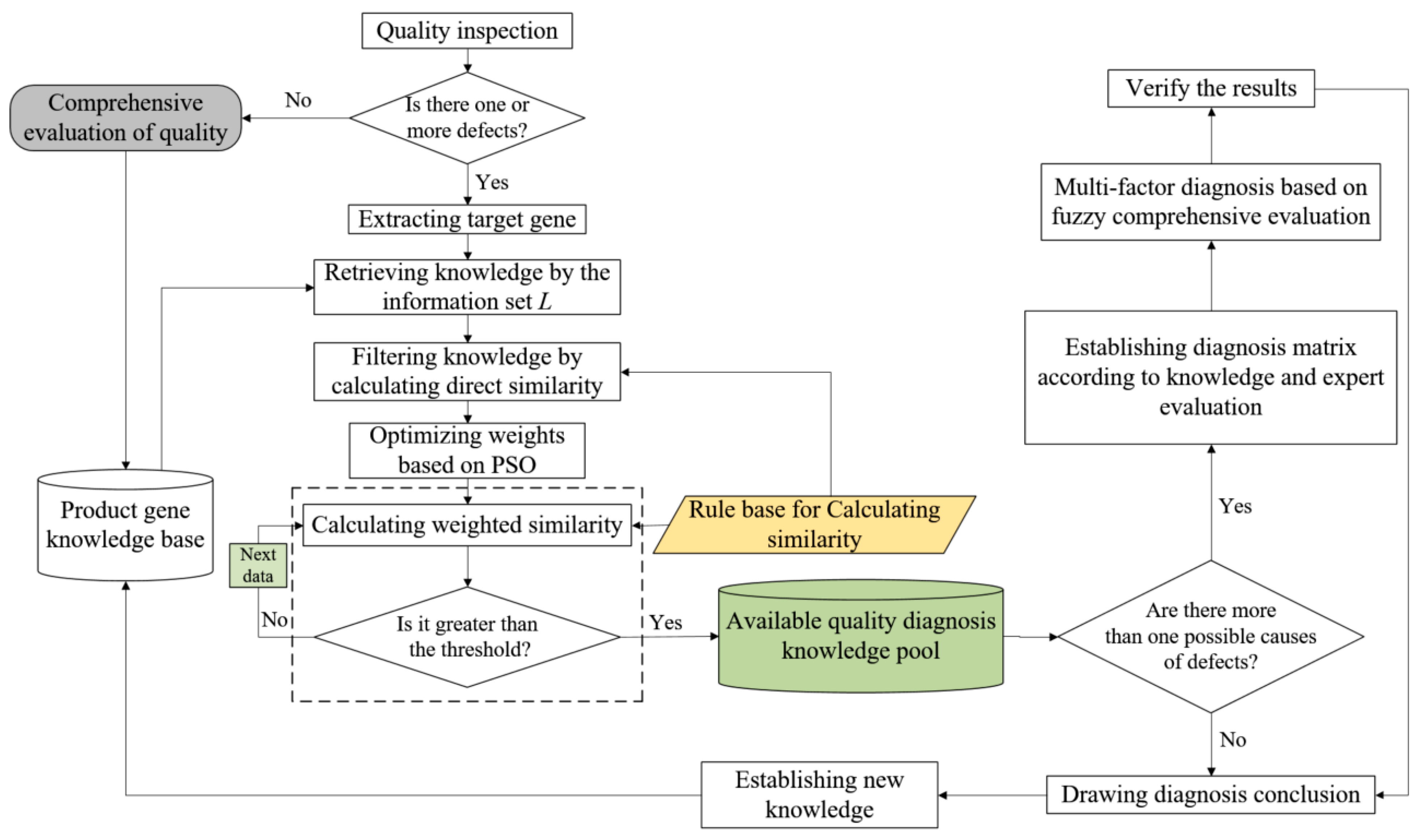
In the framework, the proposed method includes two parts: product gene theory and the quality defect diagnosis method. The former is the application foundation of the latter. As shown in Figure 1, the product gene model and encoding method are applied to extract the target gene. The similarity calculation rule is applied to retrieve and filter knowledge genes from the product gene knowledge base, where direct similarity and synthetic similarity are used to filter knowledge genes. In addition, a PSO is developed to optimize the weights of elements in the target gene for calculating synthetic similarity. The fuzzy comprehensive evaluation method is applied to get diagnostic results (i.e., quality defects diagnosis shown in Figure 1). Finally, these results will be validated according to the actual manufacturing information of the defective product, and then a new knowledge gene will be established with the encoding method. The contributions of this study can be summarized as follows:
(1) A quality gene model and a corresponding encoding method are developed. Compared with the existing studies, the model provides good flexibility in application.
(2) Both similarity evaluation rule and fuzzy comprehensive evaluation are applied in the study to meet the characteristic of many-to-many between quality defects and quality influence factors.
(3) An optimization of weights based on PSO is developed in the study to improve the calculation method of similarity and obtain more accurate diagnostic results.
The rest of this paper is organized as follows. Section 2 gives an overview of the related work about product gene theory and its application. Section 3 defines the product gene model, encoding method, similarity calculation rule, and the mode of evolution. Then, a quality defects diagnosis method based on the proposed product gene model and methods is explained in Section 4. In Section 5, an experiment about bearing spacer in an M5018A roller press is applied to illustrate the method proposed in Section 4. Finally, conclusions are drawn in Section 6.

2. Related Work

Genetic engineering comes from the field of biology. It is introduced into the manufacturing field for its similarity with products which have been studied in the literature [26,27,28]. To increase the efficiency and quality of designing, Shang et al. [29] introduced the concept of the functional surface as the information carrier to link product function and structure together. They described a product genetic model to represent and organize product information. Feng et al. [30] established a mechanism chromosome model, which is constituted by a mechanism chromosome relationship graph and mechanism chromosome matrix. Focusing on the diversity and complexity of machine tools design, Zhao et al. [31] proposed a novel gene recombination method based on a complex network; the method extracts the assembly components of machine tools as the structural genes for defining the extraction rules of network elements. Zhu et al. [32] proposed a designing method based on gene recombination and integrated with reverse engineering; in their study, the product gene is divided into function gene and structure gene. The studies mentioned above focus on improving the efficiency and quality of product design, which is the main application field of the product gene. These results provide sufficient application basis for other fields, including quality diagnosis. However, most of the existing studies ignored the dynamic quality information covering production environment, workers, state of machine tools, and so on in the manufacturing process. Focusing on the problem of quality defects diagnosis in the manufacturing process for large equipment, Sun et al. [5,33] proposed a quality diagnosis method based on a quality gene model to analyze the causes of quality defects, which is effectively applied in building equipment-manufacturing enterprises. Li et al. [2] proposed a quality evaluation method to predict and diagnose product quality based on the product gene.
In summary, substantial progress has already been made in the existing researches of product gene theory, but the following issues are still needed to be dealt with:
(1) The existing research about product genes focuses mainly on the product design of structure, assembly, function, performance, and so on. Therefore, the product gene information models cannot meet the demands of quality diagnosis in comprehensiveness and dynamism.
(2) Most of the existing gene models take one product or one component as the minimum unit of the model, but most of the parts or products are different in terms of standards, materials, demands of functions, and performance in the manufacturing enterprise of large equipment, so the gene model proposed in the existing literature have limited reusability.
(3) Little research developed or integrated the diagnosis method based on product gene theory with the characteristic of many-to-many between quality defects and quality influence factors in some cases.

3. Product Gene Theory

In manufacturing enterprises of large equipment, the customization degree of a product is very high, thus most products or parts are different. Considering this characteristic, establishing a general model for describing product quality information is of great importance. Geometrically, a point is the smallest entity, followed by a line, surface, part, and component. In mechanical structure, points and lines are cumbersome and inconvenient to express a quality unit. Compared with solid parts and components that are the information unit of quality model [5,33], the surface is the most suitable unit to describe quality information and to provide a general information model for quality management [29]. To describe the quality information reasonably and to improve its applicability by considering the characteristics of large equipment and its manufacturing process, a product gene model based on processing surface for dynamic quality control is developed in this paper.
Definition 1.
Processing surface: It is not a new concept to the mechanical engineering field with a different perspective. In this paper, a processing surface is a unit that is formed after a series of manufacturing processes, and it is also a continuous surface with some certain functions, which include assembly, load bearing, improving performance, and so on.

3.1. Product Gene Model for Dynamic Quality Control

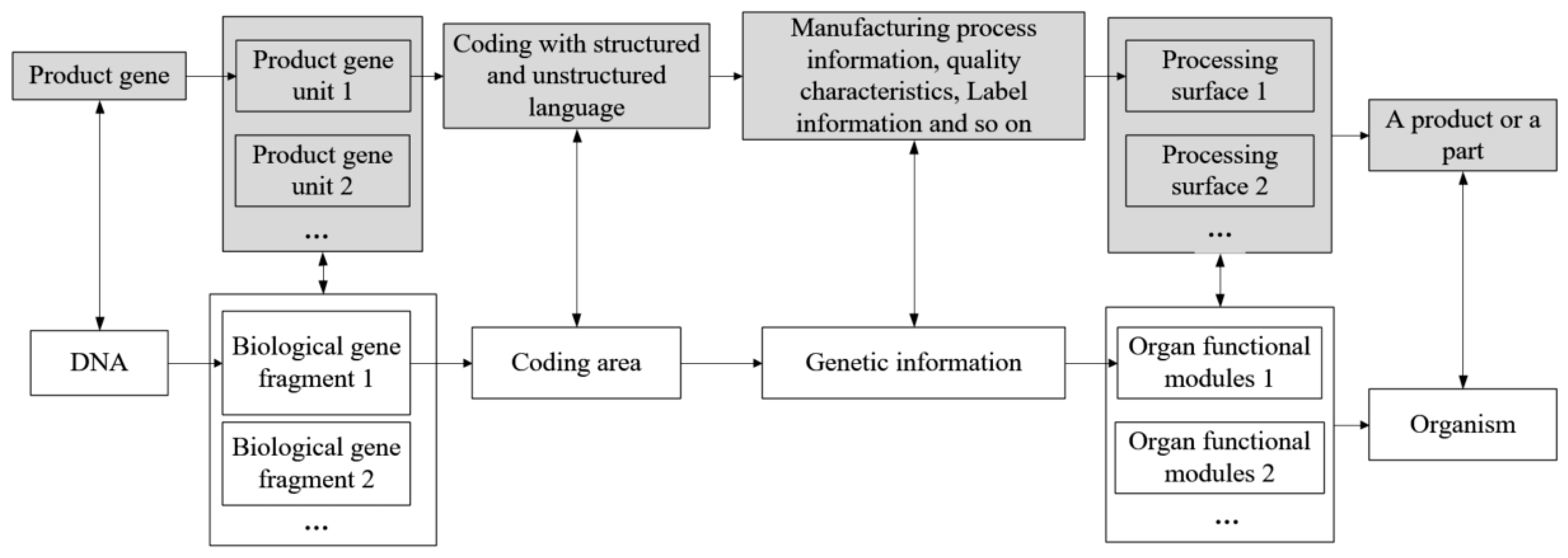
Biologically, a gene is a segment of DNA with specific genetic information. DNA consists of four nucleotides which include A, T, C, and G [34]. The sequence of these nucleotides determines the features of an organism. Therefore, a gene is also a group of specific nucleotide sequences which determines a set of specific characteristics [29]. Besides, genes can transmit genetic information to the next generation [5]. Similar to an organism, a processing surface is a basic unit to form its one product or one component. Correspondingly, a product gene unit describes the genetic information of a special surface which determines a set of features, the gene of one product or one part which consists of a set of gene units. Corresponding to biological genes, the relationship between biological gene and product gene for dynamic quality control of large equipment is shown in Figure 2.
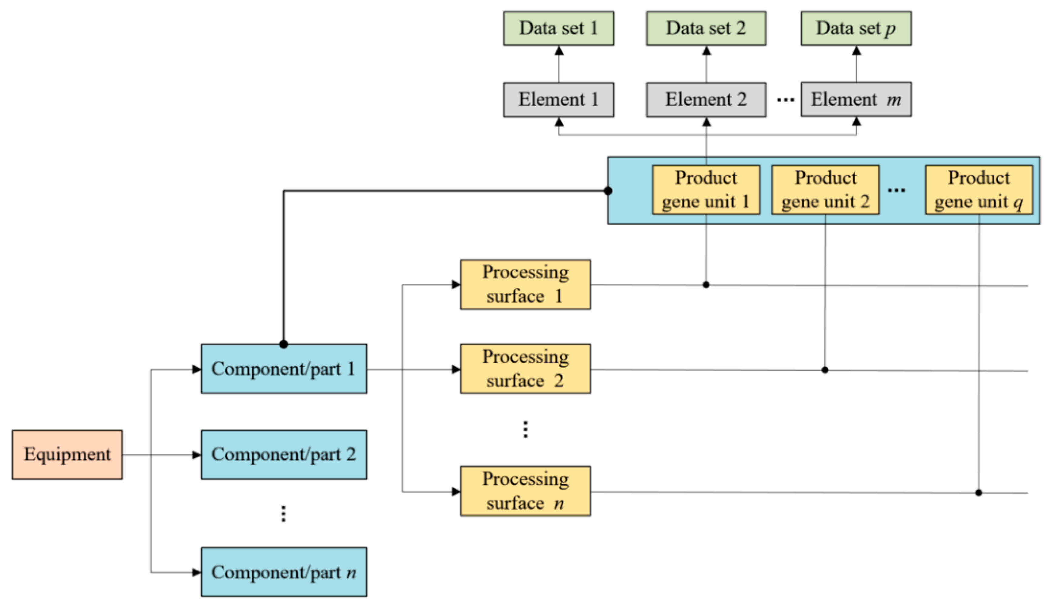
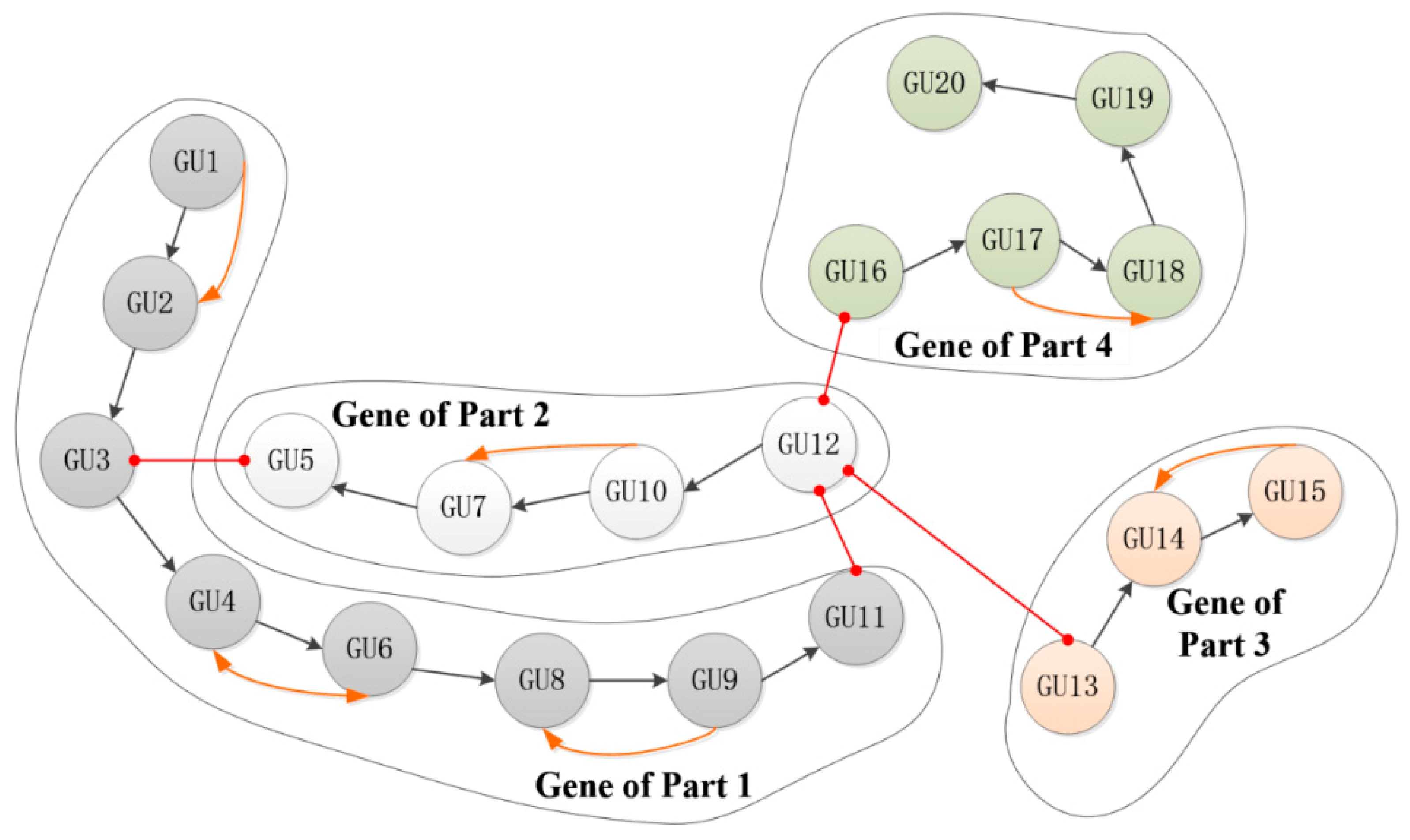
In addition, the gene of one product or one part is multi-level and interrelated, it can be explained by the descriptions as shown in Figure 3 and Figure 4. GUq in Figure 4 represents gene unit q. Different lines represent different relationships among the gene units, which include assembly relationship, influence relationship, and sequence relationship.
Considering the characteristics mentioned above, the definitions of product gene based on the processing surface are performed as follows:
Definition 2.
Product gene unit based on processing surface: In this study, we express the product gene of a surface with a model which consists of 6 sets as the expression (1). According to the corresponding relationship between product structure and product gene as shown in Figure 3, the gene of one product or one part can be expressed by expression (2).
G U = ( L , C , P , I , R , P E )
P G = { G U ( 1 ) , G U ( 2 ) , , G U ( q ) }
whereL, C, P, I, R,andPErepresent Label Information Set, Quality Characteristics Information Set, Processes Information Set, Quality Influence Factors Set, Interrelated Information Set and Quality Performance Information Set respectively.
Definition 3.
Label Information Set L: It is used to describe the adscription information of a processing surface and expressed by L = (UID, EC, PC, SC). Here, UID represents the unique code of gene unit, EC represents the code of equipment which is composed of the code of equipment name and equipment type, PC represents the code of part which is composed of the code of part name and part type, and SC represents the code of surface name and surface type.
Definition 4.
Quality Characteristics Information Set C: C = (C1, C2, C3, …, Ca). It describes the size, precision, and feature properties of a processing surface. Here, the properties include length, width, radius, screw-pitch, roughness, hardness, and so on, of which each is represented by a Ci.
Definition 5.
Process Information Set P: P = (P1, P2, P3, …, Pb). It describes the information of processing types and methods of a processing surface. Here, Pi consists of the allowance of one side and the processing mode of process i, which is shown by Pi = (AWi, PMCi).
Definition 6.
Quality Influence Factors Set I: I = (MAT, I1, I2, I3, …, Ic). Quality influencing factors mainly include operator, equipment, material, process, measurement, and environment (5M1E) [35]. Therefore, 5M1E is the basis of the quality influence factors set. In Quality Influence Factors Set, Ii = (CWi, TMi, MAi, ETEMi, HMDi, IMi, TLi, PTEMi) represents the information of influence quality of process i. Here, the eight symbols in Ii represent the capability of the worker, type of machine, age of machine, temperature of environment, humidity of environment, method of detection, time of heat treatment, and temperature of heat treatment, respectively. The number of quality influence factors involved in different processes are different. MAT represents the material of target gene unit. The structure of I has strong adaptability in meeting the demands of extensive collaborative manufacturing of large equipment.
Definition 7.
Interrelated Information Set R: It contains three kinds of interrelated information, i.e., assembly relationship, influence relationship, and sequence relationship. Therefore, it can be represented by a 3-tuple as R = (AR, IR, NR). Here, AR contains the codes of surfaces which have assembly relation with the target surface, IR contains the codes of surfaces which would influence the quality of target surface and NR contains the codes of surfaces defining the sequence of the target surface in a part just like a part in a piece of equipment.
Definition 8.
Quality Performance Information Set PE: PE describes the performances of one gene unit or one part. It is represented by PE = (pe1, pe2, pe3, …, ped) which contains a set of strings which represent different defects and different states of the target surface.

3.2. Encoding Method of Product Gene

Definitions described above explained the structure of a product gene unit. To apply it, a reasonable encoding solution is necessary to be established. Focusing on the problem, some typical encoding methods have been developed. For instance, Shang et al. [29] proposed a feature-oriented encoding scheme based on the generalized positioning principle (GPP) by taking the functional surface as the basic gene carrier. Cao et al. [36] presented an encoding approach for part and product series. Sun et al. [5] proposed a two-level quality gene encoding method for quality diagnosis. Looking at the product quality evaluation problem, Li et al. [2] developed an encoding method based on letters.
Large equipment contains a large quantity of heterogeneous quality information. Its encoding method of information should avoid information misunderstanding caused by inconsistent names, descriptions, and classifications to the greatest extent for its excellent application performance. Therefore, based on the principles of uniqueness, classification, high adaptability, integrity, and efficient retrieval, a sectional encoding method is developed in this paper to describe and store the information of elements in the product gene. The characteristics of this method are as follows:
(1) Each element consists of three segments of data, they are separated with “#.” Therefore, an element can be expressed by EL = (ECS#EVS#EMS), where ECS, EVS, and EMS represent the code of an element, the value set of attributes of the element and the metadata set corresponding to EVS. Here, the data format of EVS corresponding to an ECS is fixed. EMS describes types of values in corresponding EVS. EVS and EMS can be expressed by EVS = (evs1, evs2, …, evse) and EMS = (ems1, ems2, …, emsf) respectively. If values in EMS are the same, then EMS = ems. This approach can effectively reduce the number of encodings.
(2) The first segment of each element is encoded according to its information set and element type. The values of the second segment uniformly represented by strings for improving the applicability of the encoding method. Then these values can be appropriately used according to the coding of the last paragraph.
Table 1 shows the main data types in EMS. Five data types are applied to describe the values of EVS of the product gene. For instance, the information of size and precision are defined with continuous numeric values, the information of measuring methods are defined with option values, the information of capabilities of workers are defined with discrete values, and so on.
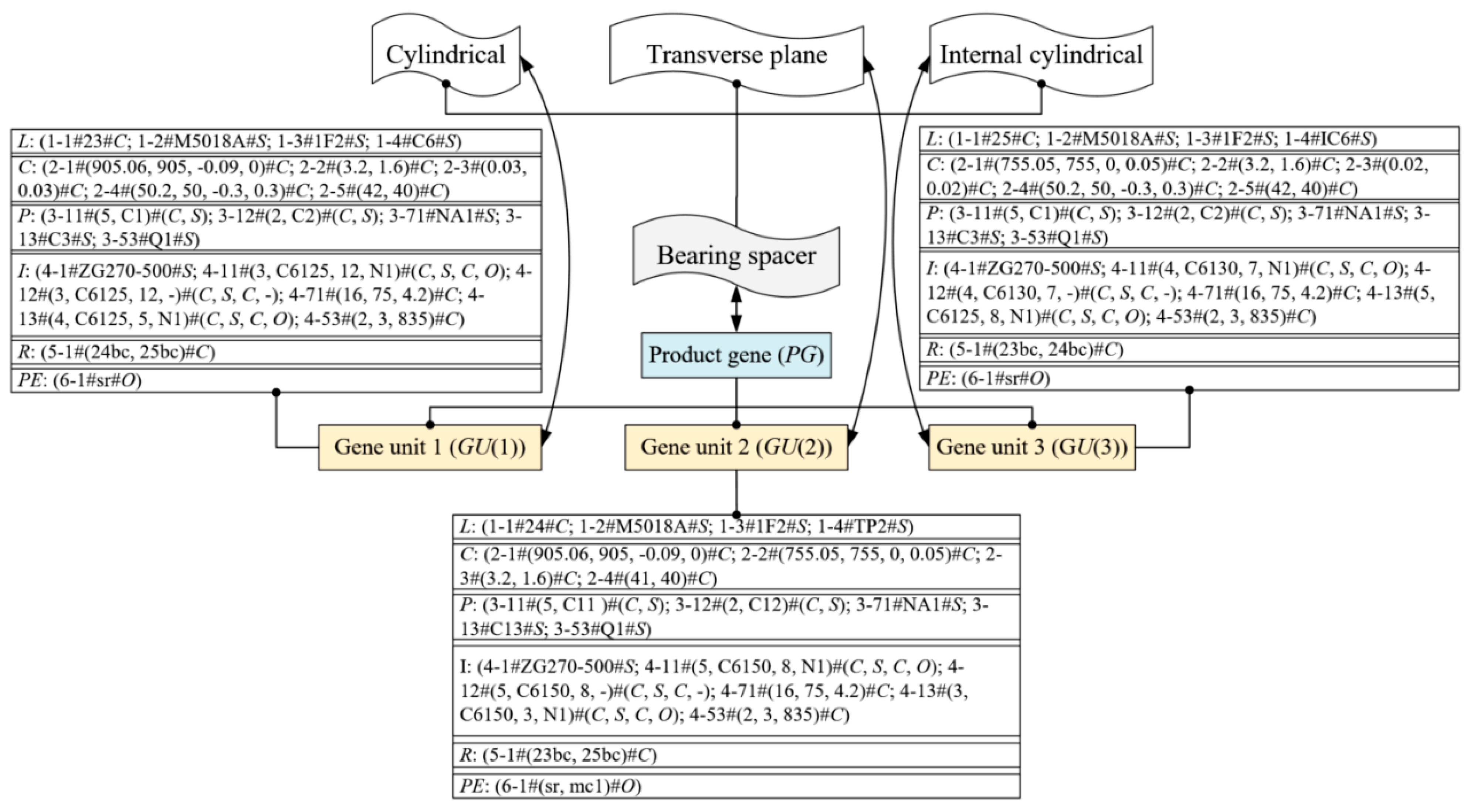
Assuming what is shown in Figure 5 is the product gene of a bearing spacer, according to the definitions in Table 1, the product gene of this bearing spacer should consist of three gene units. The meanings of codes in GU (1) are explained in Table 2.
As shown in Table 2, the code of one element consists of three segments split by “#.” The first segment of the element describes its code, the second segment describes its related values of attributes, and the third segment describes the type of each value. For instance, in the “4-1#ZG270-500#S”, the “4” indicates that the code belongs to I, the “4-1” represents the element of material, the “ZG270-500” is the material, and the “S” indicates that the type of “ZG270-500” is a string. In the “4-11#(3, C6125, 12, N1)#(C, S, C, O)”, “4-11” represents the rough turning, the “(3, C6125, 12, N1)” indicates that the capability of worker is “3”, the machine type is “C6125”, the age of the machine is 12 years, and the inspection method of rough turning is the conventional method, and the “(C, S, C, O)” describes the types of values of the “(3, C6125, 12, N1)”.

3.3. Similarity Calculation Rule

To apply product gene theory, a similarity calculation rule is developed to measure applicability of diagnosis knowledge in product gene knowledge base in a specific case. Its definition has been described in the literature [5]. Here, the product gene knowledge base is the information basis of application of product gene theory. It is defined as follows:
Definition 9.
Product Gene Knowledge Base: It consists of a great quantity of product gene knowledge of quality, the data come from the historical data of quality management and control. The product gene knowledge is similar to a product gene, and its gene unit consists of 7 sets, as shown in expression (3).
K G U = ( L , C , P , I , R , P E , K C L )
where the first six sets are similar to the sets inGU, KCLdescribes the evaluation and diagnosis conclusions which are expressed byKCL = (kcl1, kcl2, kcl3, …, kclg). The encoding method of KGU is the same as GU.
In this study, if ECS of an element and value of SC in the target gene are the same as they are in the reference gene, the values of them can be used to calculate similarity. Considering the data types as shown in Table 1, to calculate the similarity between the elements in target gene and the corresponding elements in the reference gene, the string similarity, numerical similarity, option similarity, and discrete similarity are defined to calculate the similarity, and they are explained as follows:
(1) String similarity
The string similarity is measured by matching degree between two strings. The calculation method is expressed as follows:
δ ( S t r A , S t r B ) = L e n ( S t r A ( i ) = = S t r B ( i ) ) m a x { L e n ( S t r A ) , L e n ( S t r B ) )
where StrA and StrB represent values of attributes which are strings in the target gene and reference gene, respectively. StrA(i) and StrB(i) represent the ith character in StrA and StrB respectively. Len(StrA(i)==StrB(i)) represents the number of the same characters between StrA and StrB. Len(StrA) and Len(StrB) represent the length of StrA and StrB, respectively.
(2) Numerical similarity
The similarity between two continuous values can be calculated in different ways for a different type of attributes. If the attribute is not in information set C, then the similarity can be calculated as follows:
δ ( N u m A , N u m B ) = { m i n { | N u m A | , | N u m B | } m a x { | N u m A | , | N u m B | } N u m A × N u m B > 0 0 m a x { | N u m A | , | N u m B | } > 0 ,   N u m A × N u m B 0 1 N u m A = N u m B = 0
where NumA and NumB are values of attributes which are both continuous in target gene and reference gene.
In information set C, an element can be expressed by EL_C = SC#(NV1, NV2, NV3, NV4)#C, where NV1 represents the actual value, NV2 represents the design value, NV3 represents the lower deviation, NV4 represents the upper deviation. Their types of values are all continuity. Considering their different roles, the calculation methods of them are defined as follows:
The similarity between an NV2 or NV3 or NV4 in target gene (NVA2 or NVA3 or NVA4) and the corresponding NV2 or NV3 or NV4 in reference gene (NVB2 or NVB3 or NVB4) is calculated by Equation (5).
If the values of NVA3, NVA4, NVB3, and NVB4 are all null, then the similarity between an NV1 in target gene (NVA1) and the corresponding NV1 in reference gene (NVB1) is expressed as follows:
δ ( N V A 1 , N V B 1 ) = { m i n { | N V A 1 N V A 2 | , | N V B 1 N V B 2 | } m a x { | N V A 1 N V A 2 | , | N V B 1 N V B 2 | } ( N V A 1 N V A 2 ) × ( N V B 1 N V B 2 ) > 0 0 ( N V A 1 N V A 2 ) × ( N V B 1 N V B 2 ) 0 , m a x { | N V A 1 N V A 2 | , | N V B 1 N V B 2 | } > 0 1 N V A 1 N V A 2 = N V B 1 N V B 2 = 0
In this equation, the value of similarity is determined by the difference between the actual value and the design value. Considering the design accuracy, it can more accurately reflect the difference between the target value and the reference value than Equation (5). For example, the design value of hardness of a part is 40; it means that the actual hardness of the product should not be less than 40 to qualify. If the actual hardness (target value) is 36 and a reference value is 42, the similarity is 36/42 = 0.86 according to Equation (5), while the similarity is 0 according to Equation (6). Here, the target value does not meet the requirements, while the reference value meets the requirements. Obviously, 0 is better than 0.86 in reflecting their similarity. Therefore, Equation (6) is applied under the conditions above.
If the values of NVA3, NVA4, NVB, and NVB4 are not null, then the similarity between an NV1 in target gene (NVA1) and the corresponding NV1 in reference gene (NVB1) is expressed as follows:
δ ( N V A 1 , N V B 1 ) = { m i n { | D A | , | D B | } m a x { | D A | , | D B | } D A × D B > 0 , ( D A < 1 , D B < 1 )   or   ( DA > 1 , DB > 1 ) 0 ( D A × D B 0 , m a x { | D A | , | D B | } 0 )   or   ( D A > 1 , 0 < D B < 1 )   or   ( 0 < DA < 1 , DB > 1 ) 1 D A = D B = 0
D A = N V A 1 ( N V A 2 + N V A 3 ) N V A 4 N V A 3
D B = N V B 1 ( N V B 2 + N V B 3 ) N V B 4 N V B 3
where DA is the deviation degree of value in target gene and DB is the deviation degree of value in the reference gene. NVA3 and NVB3 are reference values. Similar to Equation (6), the calculation method as shown in Equations (7)–(9) can obtain a more accurate value of similarity than Equation (5).
(3) Option similarity
The option similarity is measured by the matching state between two values which are optional or Boolean. The calculation method is expressed as follows:
δ ( O p t A , O p t B ) = { 0 O p t A O p t B 1 O p t A = O p t B
δ ( B l A , B l B ) = { 0 B l A B l B 1 B l A = B l B
where OptA is an optional value of an attribute in the target gene and OptB is an optional value of an attribute in the reference gene. BlA is a Boolean value of the attribute and BlB is a Boolean value of an attribute in the reference gene.
(4) Discrete similarity
Discrete value is an uncontinuous value and the value corresponds to a certain interval or one of the predefined values. Different from option and Boolean values, the discrete value can be used to do mathematical calculations. The discrete similarity is expressed as follows
δ ( D r e 1 , D r e 2 ) = 1 | D r e 1 D r e 2 | D r e m a x ( j ) D r e m i n ( j )
where Dre1 is a discrete value of an attribute in the target gene and Dre2 is a discrete value of an attribute in the reference gene. Dremax(j) is the maximum value of the jth discrete variable and Dremin(j) is the minimum value of the jth discrete variable. Each of them represents a certain interval or one of the predefined values. For instance, the capabilities of workers can be divided into several levels with an expression of WLS = {1, 2, 3, 4, 5, 6, 7}, “7” represents the most proficient level while “1” represents the least skilled level. Therefore, Dremax(j) is “7” and Dremin(j) is “1”. If Dre1 is “5” and Dre2 is “3,” then δ(Dre1, Dre2) = 0.67.
In addition, the values of attributes “1-1” and “5-1” are only used to retrieve relevant data from the product gene knowledge base without calculating similarity.

3.4. Evolution Mode of Product Gene

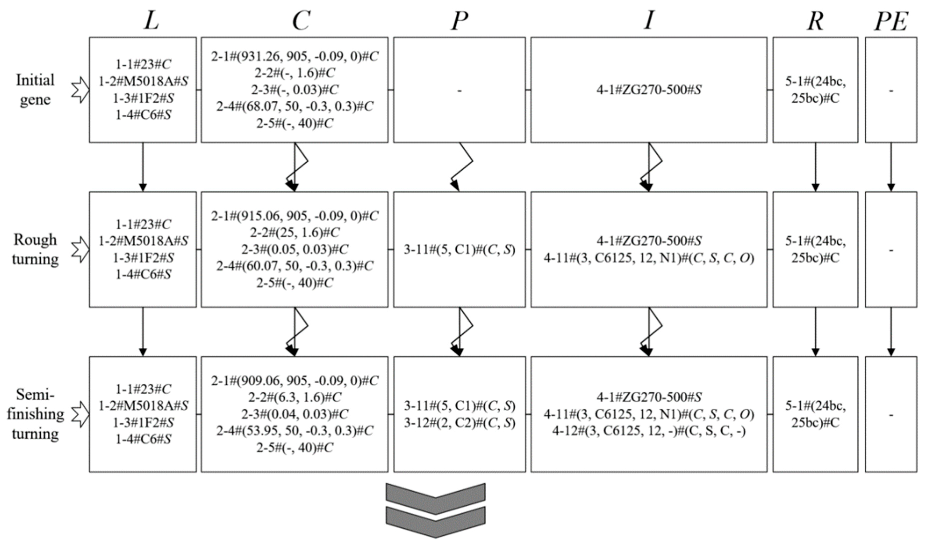
Similar to biological genes, the product gene is also hereditary, and its evolution happens along with the manufacturing process of a product or a part. The initial codes of the product gene come from the design data. In the manufacturing process, some quality information is transmitted as genetic information to the next generation while other information changes during the manufacturing process. The evolution process of GU (1) as shown in Table 2 is shown in Figure 6.
In the evolution process of product gene, some information is new and some information is inherited from the changes of other information, its essence is a gradual process of product formation. For instance, in Figure 6, the ”3-11#(5, C1)#(C, S)” is generated after rough turning. The “2-5#(-, 40)#C” is inherited to the next generation. The “2-1#(931.26, 905, -0.09, 0)#C” becomes “2-1#(915.06, 905, -0.09, 0)#C” after rough turning.
In summary, the product gene model, encoding system, similarity calculation rule together with evolution mode of product gene provide the theoretical as well as a methodological basis for describing, tracking, and applying quality information. It is of great significance to realize dynamic quality description and controlling in the manufacturing process.

4. Quality Diagnosis Method for Manufacturing Process

Product gene theory has been applied to quality defects diagnosis [5]. The calculation method of synthetic similarity between the target gene and the reference gene is applied to find the applicable diagnosis knowledge in product gene knowledge base. It ignores the characteristic of many-to-many between quality defects and quality influence factors in many cases. Besides, the weight of each element is set directly, which may lead to inaccurate diagnosis result. Therefore, a quality defects diagnosis method based on similarity and fuzzy comprehensive evaluation is developed in this study with the theory and methods proposed in Section 3 of this paper, and the PSO is applied to optimize the weights of elements of product gene. Figure 7 shows the process of quality defects diagnosis method.
In the process, the quality diagnosis method based on product gene theory contains two parts covering filtering knowledge and fuzzy comprehensive evaluation for multi-factor diagnosis. Here, the effective data of the target gene should be extracted from the database for modeling the data and removing useless information. The detail elaboration of filtering knowledge will be shown in Section 4.1, with the second parts of which the fuzzy comprehensive evaluation being shown in Section 4.2.

4.1. Filtering Method of Product Gene Knowledge

The related parameters and variables are summarized as follows:
mNumber of related gene units
kIndex of a gene unit
nk, wkNumber of elements of gene unit k, the weight of gene unit k
pk, pk, wpkIndex of an element in gene unit k, corresponding index in a knowledge gene unit, weight the element
n(pk)Number of attributes of element pk
i(pk), i(pk)Index of an attribute in element pk, corresponding index in a knowledge gene unit
SD(PG, KPG)Direct similarity between target gene (PG) and reference gene (KPG)
SD(GU(k), KGU(k))Direct similarity between gene unit k in PG and corresponding gene unit in KPG
S(PG, KPG)Synthetic similarity between PG and KPG
S(GU(k), KGU(k))Synthetic similarity between gene unit k in PG and corresponding gene unit in KPG
δ(E(pk), KE(pk))Similarity between element pk in PG and the corresponding element in KPG
δ(A(i(pk)), KA(i(pk)))Similarity between attribute i(pk) in PG and the corresponding element in KPG
TS, TSSThreshold of direct similarity, the threshold of synthetic similarity
SD(GU(k)(PE), KGU(k)(PE))Direct similarity between the information set PE in GU(k) and corresponding information set in KGU(k)
As shown in Figure 7, there are two methods that are applied to filter the product gene knowledge after retrieving knowledge from database. The two methods are explained in Section 4.1.1 and Section 4.1.2, respectively. Here, retrieving knowledge can be realized by database technology; it has a very high data processing efficiency.

4.1.1. Filtering Knowledge by Calculating Direct Similarity

We can get different kinds of knowledge genes by retrieving and some useless data is also included. Besides, in some cases, the number of knowledge genes is large. It is difficult to process and analyze the data. Therefore, it is necessary to filter knowledge genes with similarity. However, the weight cannot be determined for the time being. So it is an efficient method to filter knowledge genes with direct similarity for further application, where direct similarity is the value of similarity without considering weights. The direct similarity between the target gene and the reference gene is calculated as follows:
S D ( P G , K P G ) = k = 1 m S D ( G U ( k ) , K G U ( k ) ) n k k = 1 m n k
S D ( G U ( k ) , K G U ( k ) ) = p k , p k = 1 n k δ ( E ( p k ) , K E ( p k ) ) n k
δ ( E ( p k ) , K E ( p k ) ) = i ( p k ) , i ( p k ) = 1 n ( p k ) δ ( A ( i ( p k ) ) , K A ( i ( p k ) ) ) n ( p k )
Equation (13) is the calculation method of the direct similarity, and it is explained by Equations (14) and (15). Here, if SD(PG, KPG)>TS, then the knowledge gene is a relevant reference gene of quality defects diagnosis.

4.1.2. Filtering Knowledge by Calculating Synthetic Similarity

To get knowledge genes more accurately, calculating synthetic similarity is important for further filtration, where synthetic similarity is the value of similarity with the consideration of weights. The synthetic similarity between the target gene and the reference gene is calculated as follows:
S ( P G , K P G ) = k = 1 m S ( G U ( k ) , K G U ( k ) ) w k
S ( G U ( k ) , K G U ( k ) ) = p k , p k = 1 n k δ ( E ( p k ) , K E ( p k ) ) w p k
k = 1 m w k = 1
p k = 1 n k w p k = 1
Equation (16) is the calculation method of the synthetic similarity, and it is explained by Equations (15) and (17). Equations (18) and (19) are the constraint conditions. Here, if S(PG, KPG)>TSS, then the knowledge gene is an available reference gene.
Optimizing weights. A dynamic optimization method of weights based on PSO is developed in this study. PSO is a population evolutionary algorithm (EA) inspired by social behavior of bird flocking. Compared with other algorithms, it is more robust as it can work with limited information such as the fitness evaluation of each particle [37]. Besides, the encoding method of PSO can meet the demands of continuous or discrete variable values, therefore, it can be used to solve approximation of extremum and manufacturing resource combinatorial optimization (MRCO) problems [38,39].
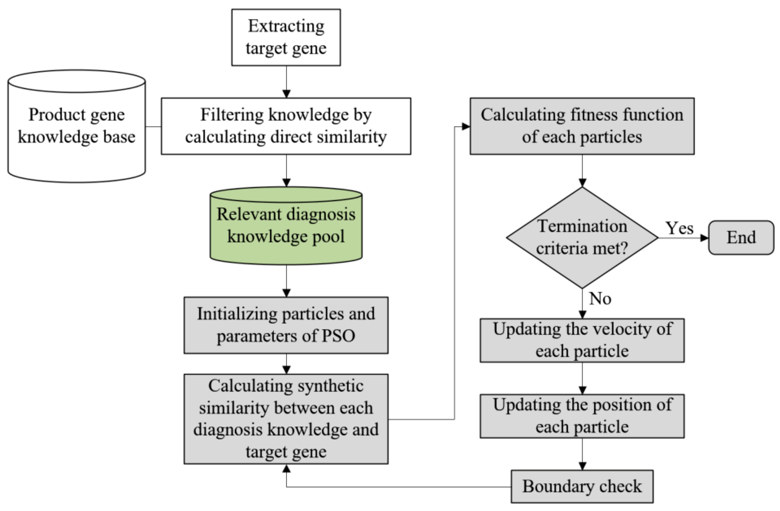
For the reasons mentioned above, PSO is applied to optimize weights in calculating the synthetic similarity between the target gene and the reference gene. Figure 8 illustrates the flowchart of the optimization method of weights with PSO. The optimization process and encoding method of PSO have been explained in the literature [1] and the particles in this study are continuous codes.
According to Equations (16)–(19), the calculation method of synthetic similarity and constraints of weights are expressed as follows:
S ( P G , K P G ) = k = 1 m ( p k , p k = 1 n k δ ( E ( p k ) , K E ( p k ) ) w p k ) w k = p = 1 n δ ( E ( p k ) , K E ( p k ) ) w p
w p = w p k * w k
p = 1 n w p = 1
n = k = 1 m n k
where n refers to the total number of elements, p refers to the index of an element, wp refers to the element p in the target gene. Therefore, a particle in PSO can be described with a set of weights [x1, x2, …, xp, …, xn] corresponding to the elements in the target gene and wp = xp. The fitness function f(x) of each particle is expressed as follows:
f ( x ) = i = 1 l 1 S ( P G , K P G i ) × S D ( P G ( P E ) , K P G i ( P E ) ) j = 1 l 2 S ( P G , K P G j ) = p = 1 n ( i = 1 l 1 ( δ ( E ( p ) , K E i ( p ) ) × S D ( P G ( P E ) , K P G i ( P E ) ) ) j = 1 l 2 δ ( E ( p ) , K E j ( p ) ) ) w p
S D ( P G ( P E ) , K P G i ( P E ) ) ) = k = 1 m S D ( G U ( k ) ( P E ) , K G U ( k ) ( P E ) )
l 1 + l 2 = l
w p = x p p = 1 n x p
where l is the total number of knowledge genes in relevant diagnosis knowledge pool as shown in Figure 8. l1 is the number of knowledge genes which meet the condition SD(PG(PE), KPGi(PE))>0, l2 is the number of knowledge genes which meet the condition SD(PG(PE), KPGj(PE)) = 0. KPGi and KPGj represent the knowledge gene in the relevant diagnosis knowledge pool. It means that a knowledge gene should be valued if the similarity between the PEs of the knowledge gene and that of the target gene is greater than 0.

4.2. Fuzzy Comprehensive Evaluation for Multi-Factor Diagnosis

Fuzzy comprehensive evaluation (FCE) is a comprehensive decision-making methodology for solving multi-variable problems in a complex decision process [40]. Particularly, it is the process that a large number of related factors are covered comprehensively and multiple objectives are taken into account together to obtain reference results [41]. The characteristics of FCE can be summarized as follows: First, it should be applied to problems with multi-factor; second, its result is a fuzzy set rather than a determined value [42,43]. Therefore, FCE is an effective and applicable method in accordance with the characteristic of many-to-many between quality defects and causes. The main process of FCE are explained in detail as follows:
Calculating membership degree. In this study, each quality defects in PEs of the target gene and the reference gene is a fuzzy factor. A fuzzy factor set consist of these factors in available quality diagnosis knowledge pool. Different factors can be categorized into different fuzzy classifications to a certain extent. The extent refers to the membership degree of a fuzzy classification for a fuzzy factor; these fuzzy classifications correspond to diagnosis conclusions in KCLs of knowledge genes in the available quality diagnosis knowledge pool.
Expert evaluation and empirical data (i.e., fuzzy statistical classification) are the two main methods to calculate the membership degree of fuzzy factors [44]. Expert evaluation determines membership degrees by multiple experts evaluating fuzzy classification of each fuzzy factor according to their experience, where the research objects of expert evaluation method are often definite, the numbers of fuzzy factors and fuzzy classifications are limited. In this paper, the research object, fuzzy factors, and fuzzy classifications are all varied. Therefore, the fuzzy statistical classification method is applied based on the available quality diagnosis knowledge pool, as shown in Figure 7. The membership function is defined as follows:
U α ( β ) = N α β / β = 1 b N α β
where α represents the index of a quality defect (fuzzy factor) and β represents the index of a cause (fuzzy classification), b represents the number of causes. Nαβ represents the frequency of occurrence of cause β when defect α occurs in the available quality diagnosis knowledge pool. It is explained with an example, as shown in Table 3.
According to the membership function, as shown in Equation (28), the membership degree of FC1 for FF1 is 5/(5+2+3) = 0.5, the membership degree of FC1 for FF2 is 2/(5+2+3) = 0.2, and so on. Here, the “5” is the times of occurrences of FF1, which is related to FC1 in available quality knowledge pool. “2” is the times of occurrences of FF2, which is related to FC1 in available quality knowledge pool.
Establishing fuzzy subset. The fuzzy factor set and fuzzy classification set are represented by two Euclidean vectors respectively as follows:
X = ( x 1 , x 2 , , x α , , x a )
Y = ( y 1 , y 2 , , y β , , y b )
where a represents the number of fuzzy factors (defects), xα refers to the fuzzy factor α and yβ is the fuzzy classification β. Therefore, the membership degrees of fuzzy factor α in each fuzzy classification are represented by fuzzy subset Uα as shown in Equation (31).
U α = ( u α 1 , u α 2 , , u α β , , u α b )
Here, uαβ represent the membership degree of FCβ for FFα. These values are determined by the method of calculating membership degree mentioned above.
Establishing defects vector and result vector. The defects set (i.e., PEs of target gene) and result set are described respectively as follows:
D V = ( d v 1 , d v 2 , , d v α , , d v a )
R V = ( r v 1 , r v 2 , , r v β , , r v b )
where rvβ represents the probability of evaluation object (i.e., the defects of the target gene) to be classified as yβ. The greater the value, yβ is more likely the cause of defects.
Determining FCE matrix. Based on available quality diagnosis knowledge pool, the defects and diagnosis conclusions described in PEs and KCLs of knowledge genes are applied to calculate the membership degree of each quality defects in each diagnosis conclusion. The FCE matrix consists of the membership degrees and expressed as follows:
R = [ r 11 r 12 r 1 b r 21 r 22 r 2 b r a 1 r a 2 r a b ]
where, R is the FCE matrix. rαβ is the membership degree of fuzzy factor α in fuzzy classification β corresponding to uαβ. It is expressed as follows:
r α β = u α β / β = 1 b u α β
Calculating diagnosis result. Based on of the FCE matrix R and defects vector DV, the comprehensive evaluation result set RV is calculated as follows:
R V = D V · R = ( ( d v 1 , d v 2 , , d v α , , d v a ) / ( α = 1 a d v α ) ) · [ r 11 r 12 r 1 b r 21 r 22 r 2 b r a 1 r a 2 r a b ]
The symbol “●” represents the fuzzy operator. Some composite methods including M(∧,∨), M(●,∨), M(∧, +), M(+, ●), and so on have been applied to obtain evaluation results [45]. Compared with others, the M(+, ●) method considers and retains each fuzzy factor’s contribution to the evaluation results, so it is applied in this study. The values of the fuzzy diagnosis result set RV is calculated as follows:
r v β = β = 1 b ( d v β r α β )
According to the principle of maximum membership degree, if rvβ≥1/b, the corresponding cause in Y will be identified as one of the possible causes of defects in this paper. After verification, the case of the target gene will be stored in the product gene knowledge base as new knowledge.

5. Case Study and Discussion

5.1. Data Preparation

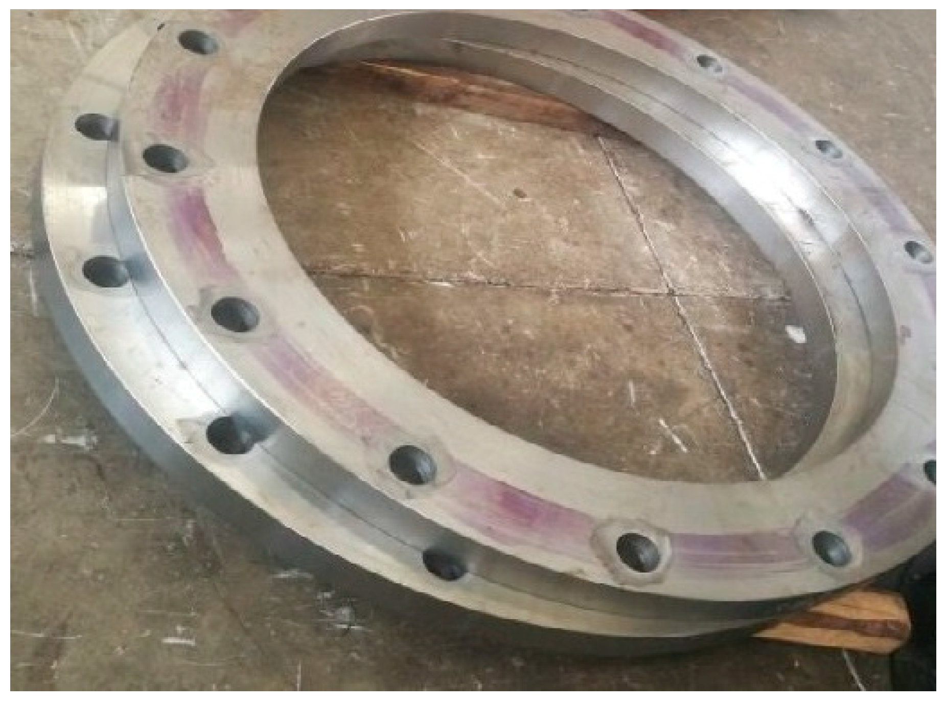
To verify the model and method proposed in this paper, bearing spacer, as shown in Figure 9 of an M5018A roller press of a building material equipment enterprise in northern China is used as an experiment. This enterprise is a large-scale manufacturing enterprise affiliated to a building material group in China; its products include roller press, cement mill, grate cooler, etc. Given the needs and characteristics of each enterprise, we have helped the group and its subordinate manufacturing enterprises to achieve in-depth informatization. In addition, due to the interconnection of information systems among these enterprises, manufacturing process data of products can be effectively managed and widely shared, which creates conditions for us to verify the theory and method of this paper.
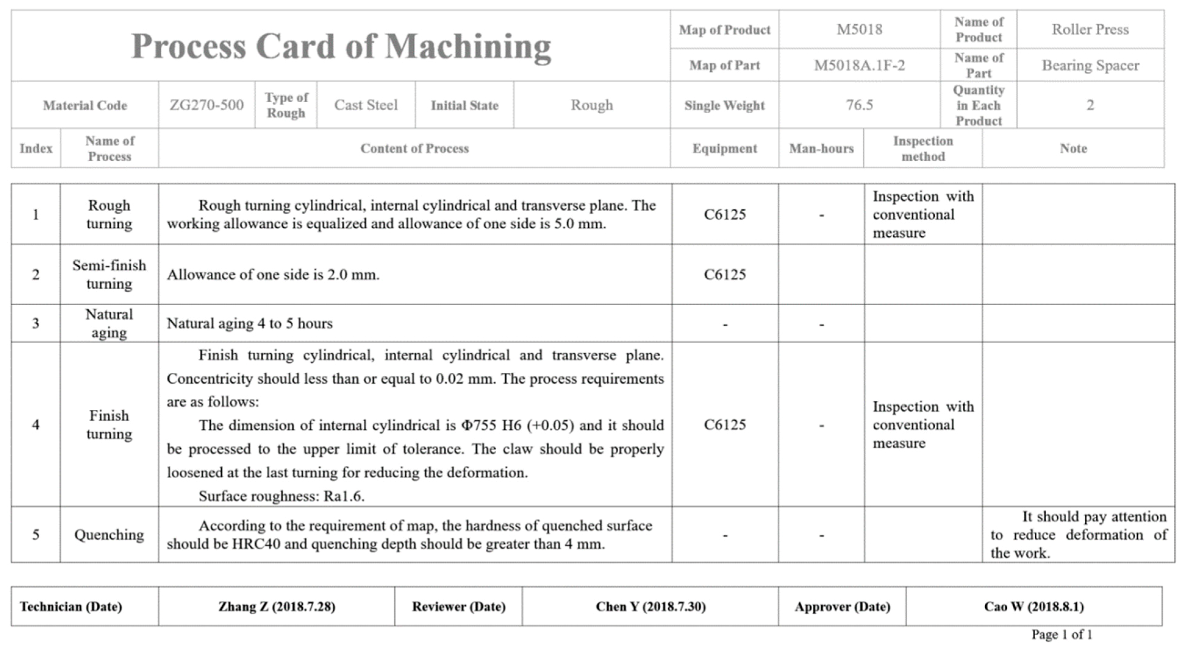
The process card of bearing spacer is shown in Figure 10. After quenching, microcracks are found on the transverse plane. In addition, the surface roughness of cylindrical, internal cylindrical, and transverse plane do not meet the requirements of design. Consequently, the causes of defects should be analyzed to avoid the same problems. In the bearing spacer, the quality of each surface is influenced by two other surfaces. Therefore, the target gene can be extracted, as shown in Figure 5, according to the process card and manufacturing process quality information.
Retrieving knowledge. In information set L, the values of elements “1-4” in the three gene units are applied to retrieve knowledge from the database. If the value of an element “1-4” in a knowledge gene equals “C6” or “IC6” or “TP2”, then the knowledge gene is taken as a result of retrieval. This method can improve the retrieval range of knowledge, and get more effective reference data. The “C6” is in GU(1), the “IC6” is in GU(2), the “TP2” is in GU(3). In addition, the information set R is used to associate the complete knowledge genes. Some of the results obtained are shown in Table 4.
Where the elements “6-1” corresponds to the information set PE and “7-1” correspond to the information sets KCL. In element “6-1,” each value represents a quality defect described by an abbreviation of its name. In element “7-1,” each value represents a cause of quality defects, which is also described by an abbreviation of its name. These abbreviations are explained in Table 5.
Due to the help of modern database technology, the information as shown in Table 4 can be quickly retrieved from the product gene knowledge base. Therefore, this method greatly improves data processing efficiency in the process of quality defect diagnosis.

5.2. Available Knowledge Acquisition

5.2.1. Filtering Knowledge Genes with Direct Similarity

To avoid the loss of valid data and the retention of invalid data, the threshold of direct similarity is set to TS = 0.7. If the direct similarity between the target gene and a knowledge gene is greater than TS, then the knowledge gene is in the relevant diagnosis knowledge pool. For instance, according to the Equations (13)–(15), the direct similarity between the target gene and the first knowledge gene, as shown in Table 4 is calculated as follows:
S D ( G U ( 1 ) , K G U ( 1 ) ) = ( 0 . 83 + 1 . 00 + 1 . 00 + 0 . 75 + 1 . 00 + 0 . 50 + 0 . 63 + 0 . 81 + 1 . 00 + 0 . 98 + 0 . 67 + 1 . 00 + 0 . 50 + 0 . 67 + 0 . 40 + 0 . 65 + 0 . 76 + 0 . 51 + 0 . 81 + 0 . 50 ) / 20 = 0.7485
S D ( G U ( 2 ) , K G U ( 2 ) ) = ( 0 . 83 + 1 . 00 + 0 . 00 + 0 . 92 + 0 . 85 + 0 . 50 + 0 . 64 + 0 . 99 + 0 . 95 + 0 . 67 + 1 . 00 + 0 . 50 + 0 . 67 + 0 . 73 + 0 . 73 + 0 . 76 + 0 . 69 + 0 . 81 + 0 . 00 ) / 19 = 0 . 6968
S D ( G U ( 3 ) , K G U ( 3 ) ) = ( 0 . 83 + 1 . 00 + 0 . 00 + 0 . 75 + 0 . 50 + 0 . 33 + 0 . 63 + 0 . 48 + 0 . 98 + 0 . 98 + 0 . 67 + 1 . 00 + 0 . 50 + 0 . 67 + 0 . 95 + 0 . 95 + 0 . 76 + 0 . 61 + 0 . 81 + 0 . 00 ) / 20 = 0 . 6700
S D ( P G , K P G ) = k = 1 3 S D ( G U ( k ) , K G U ( k ) ) n k k = 1 m n k = 0.71
Where SD(PG, KPG)>TS, the first knowledge gene should be in the relevant diagnosis knowledge pool. According to the calculation method mentioned above and TS, relevant knowledge genes, as shown in Table 6 are obtained. The corresponding values of direct similarity are shown in Table 7.
Here, 19 knowledge genes are found to be related to the target gene. After comparing the sequences of these knowledge genes, as shown in Table 6 with that of the target gene and as shown in Figure 4, we find that the information contained in these knowledge genes is similar to that of the target gene to a great extent. It indicates that the method of filtering knowledge genes with direct similarity is effective and the threshold is reasonable. As shown in Table 7, the data with bold fonts means that the corresponding knowledge genes do not contain the same defects in the target gene. Therefore, although the knowledge genes containing the same defect as the target gene are more referential, the value of other knowledge genes should not be ignored.

5.2.2. Filtering Knowledge Genes by Calculating Synthetic Similarity

According to the data in Table 7, in Equation (24), the values of l is 19, the values of l1 is 15, and that of l2 is 4. To further identify available diagnosis knowledge, the synthetic similarity is used to filter knowledge. To calculate the values of synthetic similarity between the target gene and knowledge genes as shown in Table 7, the PSO is applied to optimize the weights of elements of the target gene.
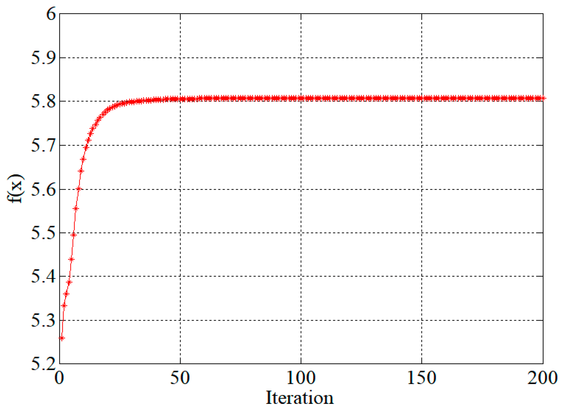
Optimizing weights. In the PSO, the initial values of weights corresponding to the initial position of a particle are set as the same value in this study. The related parameters of PSO are shown in Table 8. Besides, it will be initialized when a weight value is less than 0 or a single weight is 25% greater than the sum of all weights to guarantee the rationality of distribution of weights in the process of running PSO.
The algorithm run 30 times, the evolutionary curves of the average value of the best fitnesses (f(x)) are shown in Figure 11. It can be easily observed that the fitness is optimized to a certain extent and the algorithm converges within 50 generations. So we can conclude that the PSO is effective in the weights optimization of this study.
In particular, the solution that its best fitness is the closest to the average value of the best fitnesses is chosen to be a reasonable sequence of weights for further application. According to the results of PSO, the optimized solution is expressed by the sequence as follows:
[ 0 . 0359 , 0 . 0244 , 0 . 0432 , 0 . 0030 , 0 . 0032 , 0 . 0278 , 0 . 0135 , 0 . 0035 , 0 . 0319 , 0 . 0345 , 0 . 0022 , 0 . 0318 , 0 . 0027 , 0 . 0158 , 0 . 0164 , 0 . 0001 , 0 . 0251 , 0 . 0063 , 0 . 0201 , 0 . 0081 - 0 . 0022 , 0 . 0020 , 0 , 0 . 0131 , 0 . 0363 , 0 . 0152 , 0 . 0155 , 0 . 0408 , 0 . 0033 , 0 . 0452 , 0 . 0135 , 0 . 0401 , 0 . 0274 , 0 . 0093 , 0 . 0309 , 0 . 0142 , 0 . 0015 , 0 . 0075 , 0 . 0056 - 0 . 0092 , 0 . 0205 , 0 , 0 . 0226 , 0 . 0078 , 0 . 0105 , 0 . 0017 , 0 . 0170 , 0 . 0625 , 0 . 0425 , 0 . 0050 , 0 . 0076 , 0 . 0035 , 0 . 0431 , 0 . 0490 , 0 . 0010 , 0 . 0148 , 0 . 0069 , 0 , 0 . 0022 ]
As shown in the expression (42), the array of weights is divided into three segments, which are separated by “-“. Values in the first segment represent the weights of elements in GU(1). Values in the second segment represent the weights of elements in GU(2). Values in the third segment represent the weights of elements in GU(3). The result of weights shows that different elements have different correlations with the performance of product quality in this experiment. Based on the optimized solution, the synthetic similarities between the target gene and relevant genes as shown in Table 6 are calculated by Equations (20)–(23) and the values are shown in Table 9. The threshold of synthetic similarity is set to TSS = 0.8 for improving accuracy.
It can be easily observed that 15 values of synthetic values are greater than the threshold (TSS). Therefore, the available quality diagnosis knowledge pool consists of the corresponding 15 knowledge genes. As shown in Table 9, these available knowledge genes are marked with bold fonts. Compared with the data in Table 7, we can find that the eliminated knowledge genes in Table 9 contain the same quality defects as the target gene. It indicates that the same quality performance does not mean greater referability.

5.3. Experiment Results and Discussion

According to the data in Table 6 and Table 9, the empirical data for multi-factor diagnosis with fuzzy comprehensive evaluation are obtained as shown in Table 10, and the corresponding membership degrees as shown in Equation (45) are calculated by the approach in Section 4.2. Here, the fuzzy factor set and fuzzy classification set are expressed as follows:
X = ( sr ,   mc 1 ,   ce 1 ,   de 1 ,   de 2 ,   de 3 ,   de 4 ,   bh ,   imp ,   he 1 )
Y = ( om 11 ,   om 13 ,   mat ,   mt ,   pw 11 ,   pw 13 ,   pw 53 ,   cm 1 ,   cm 2 ,   ht 1 ,   ht 2 , tem 1 , tem 2 )
R = [ 0.11 0.09 0.06 0.14 0.11 0.06 0.03 0.06 0.11 0.11 0 0.09 0.03 0.03 0.1 0.23 0.1 0.03 0.03 0.1 0.32 0 0 0 0.06 0 0 0.09 0.14 0.14 0.09 0.14 0.14 0.14 0 0.04 0 0.04 0.04 0 0 0.17 0.32 0 0 0.17 0.17 0 0 0 0.17 0 0 0.25 0 0 0.25 0.5 0 0 0 0 0 0 0 0.14 0.29 0 0 0.14 0.14 0 0 0 0 0 0 0.29 0 0.23 0.11 0.11 0.22 0.22 0 0 0.11 0 0 0 0 0 0.09 0.14 0 0 0.09 0.14 0.09 0.04 0.09 0.09 0 0.14 0.09 0.04 0.04 0.13 0.04 0.08 0.04 0 0.13 0.37 0.13 0 0 0 0.03 0.03 0.15 0.09 0 0.03 0.15 0.12 0.06 0.19 0 0.06 0.09 ]
According to the information of the target gene and the definition of Equation (32), the defects set is encoded as
D V = ( 3 , 1 , 0 , 0 , 0 , 0 , 0 , 0 , 0 , 0 )
where each value in DV represents the frequency of a defect appeared in the target gene. For instance, the first “3” indicates that “sr” appears three times in the target gene, the first “1” indicates that “mc1” appears one time in the target gene, and so on. According to Equations (36) and (37), the result set is calculated by
R V = D V · R = ( 0.09 , 0.09 , 0.1 , 0.13 , 0.09 , 0.05 , 0.05 , 0.12 , 0.09 , 0.09 , 0 , 0.08 , 0.02 )
where each value in RV represents the degree of correlation between a cause and the defects in the target gene. For instance, the first “0.09” indicates that the possibility of attributing the defects to “om11” is 0.09, the second “0.09” indicates that the possibility of attributing the defects to “om13” is also 0.09, and so on.
Here, b = 1, then 1/b = 0.08. According to the rule defined in the last paragraph of Section 4.2 and the result set as shown in equation (47), it can be easily observed that the values of rv1, rv2, rv3, rv4, rv5, rv8, rv9, rv10, and rv12 meet the rule. Therefore, “om11”, “om13”, “mat”, “mt”, “pw11”, “cm1”, “cm2”, “ht1” and “tem1” are the possible causes of defects of the target gene. According to the data of the target gene as shown in Figure 5, the possible causes in the experiment of this study are analyzed as shown in Table 11.
Here, the causes with bold are verified to be the diagnosis results of quality defect of the bearing spacer. Among them, “om11” and “pw11” only occur on GU(1). Therefore, in this experiment, we can get the diagnosis conclusions as follows: The age of the machine of rough turning or semi-finish turning, the material of the bearing spacer, the proficiency of worker of rough turning or semi-finish turning, the structure of casting mold and the holding time of quenching are the causes of defects in GU(1); the material of the bearing spacer, the structure of the casting mold and the holding time of quenching are the causes of defects in GU(2) and GU(3).
In summary, the codes of information set KCL of GU(1), GU(2) and GU(3) in target gene should be (“om11”, “mt”, “pw11”, “cm1”, “ht1”), (“mt”, “cm1”, “ht1”) and (“mt”, “cm1”, “ht1”). Then a new diagnosis knowledge should be established based on the information and diagnosis conclusions of the target gene for further application.

6. Conclusions

To address the problem of quality defects diagnosis for large equipment, a novel quality defects diagnosis method based on product gene theory and knowledge base was developed. In the method, a product gene model and an encoding method based on processing surface were developed, whose mode of evolution was also defined. To apply the proposed product gene theory, a similarity calculation rule of attribute was proposed. A similarity evaluation rule and an optimization method of weights of elements based on PSO were addressed to filter the available knowledge of product gene from the knowledge base. Focusing on the characteristic of many-to-many between quality defects and causes, an FCE method was proposed for further localization of causes of defects. This method provides a different and valuable way for managers to optimize their quality control of manufacturing.
According to the experimental process and results in this study, it can be concluded as follows: First, the data as shown in Table 4 and Table 6 showed that the proposed product gene model and encoding method can describe the quality information of a product in large equipment manufacturing enterprises reasonably, and it also has good applicability; second, the knowledge genes obtained by filtering with direct similarity and synthetic were verified to be appropriate, so the design of the filtration method in this study is reasonable, in addition, the PSO was also proved to be n effective method to optimize weights of elements in target gene; finally, multiple factors were found to be the causes of defects in the target gene and there are differences in different gene units, thus the proposed quality defects diagnosis method can meet the characteristic of many-to-many quality defects and causes, and it also has strong flexibility. Therefore, the theories and approaches proposed in this study are effective in quality defects diagnosis.
However, there is still much to be studied further, in the future, it would be interesting to build product gene knowledge base with big data and apply product gene theory to other industries for improving its application level and value.

Author Contributions

For this article, formal analysis, S.G.; funding acquisition, S.G.; validation, X.L.; writing original draft, W.X.; writing review and editing, C.G.

Funding

This research was funded by the National Natural Science Foundation of China under Grant (51805152), the Fundamental Research Funds for the Central Universities, China (No.2016-YB-020), and the National key R & D project, China (2017YFB0404204).

Acknowledgments

The authors would like to thank Lei Wang, Rui Wu, and Baigang Du for their help in improving the model and encoding method. The authors would like to express their great appreciation for the valuable comments and constructive suggestions by the anonymous reviewers and the editor.

Conflicts of Interest

The authors declare no conflict of interest.

References

  1. Mousavi, M.; Yap, H.J.; Musa, S.N.; Tahriri, F.; Dawal, S.Z.M. Multi-objective AGV scheduling in an FMS using a hybrid of genetic algorithm and particle swarm optimization. PLoS ONE 2017, 12, e0169817. [Google Scholar] [CrossRef]
  2. Zhao, X.; Chen, G.; Yue, Q. Equipment Support Quality Management Effectiveness Evaluation based on FCE Method. Procedia Eng. 2011, 15, 4377–4381. [Google Scholar] [CrossRef] [Green Version]
  3. Li, H.; Huang, H.; Yin, Y.; Zhang, K.; Huang, P. Product Quality Evaluation Method Based on Product Gene Theory. J. Shanghai Jiaotong Univ. 2018, 23, 438–443. [Google Scholar] [CrossRef]
  4. Kamsu-Foguem, B.; Rigal, F.; Mauget, F. Mining association rules for the quality improvement of the production process. Expert Syst. Appl. 2013, 40, 1034–1045. [Google Scholar] [CrossRef] [Green Version]
  5. Sun, L.; Guo, S.; Tao, S.; Li, Y.; Guo, J. A quality diagnosis method for the large equipments base on quality gene similarity. Int. J. Adv. Manuf. Technol. 2013, 69, 2173–2182. [Google Scholar] [CrossRef]
  6. Jain, A.K.; Lad, B.K. Dynamic Optimization of Process Quality Control and Maintenance Planning. IEEE Trans. Reliab. 2017, 66, 502–517. [Google Scholar] [CrossRef]
  7. Liu, T.I.; Lee, J.; Liu, G.; Wu, Z. Monitoring and diagnosis of the tapping process for product quality and automated manufacturing. Int. J. Adv. Manuf. Technol. 2013, 64, 1169–1175. [Google Scholar] [CrossRef]
  8. Du, S.; Xi, L.; Yu, J.; Sun, J. Online intelligent monitoring and diagnosis of aircraft horizontal stabilizer assemble processes. Int. J. Adv. Manuf. Technol. 2010, 50, 377–389. [Google Scholar] [CrossRef]
  9. Zhang, X.H.; Deng, Z.H.; An, W.K.; Cao, H. A methodology for contour error intelligent precompensation in cam grinding. Int. J. Adv. Manuf. Technol. 2013, 64, 165–170. [Google Scholar] [CrossRef]
  10. Xu, F.; Liu, X.; Chen, W.; Zhou, C.; Cao, B. Ontology-Based Method for Fault Diagnosis of Loaders. Sensors 2018, 18, 729. [Google Scholar] [CrossRef] [PubMed]
  11. Zhang, K.; Dong, J.; Peng, K. A novel dynamic non-Gaussian approach for quality-related fault diagnosis with application to the hot strip mill process. J. Frankl. Inst. 2016, 354, 702–721. [Google Scholar] [CrossRef]
  12. Peng, K.; Zhang, K.; You, B.; Dong, J.; Wang, Z. A Quality-Based Nonlinear Fault Diagnosis Framework Focusing on Industrial Multimode Batch Processes. IEEE Trans. Ind. Electron. 2016, 63, 2615–2624. [Google Scholar] [CrossRef]
  13. Niu, Q. Algorithm of Multi-Causes Process Quality Diagnosis Based on Binary Tree and Intermediate Quality Indices. In Proceedings of the International Conference on Manufacturing Science and Engineering, Shenzhen, China, 30–31 March 2018. [Google Scholar]
  14. Xie, N.; Chen, L.; Li, A. Fault diagnosis of multistage manufacturing systems based on rough set approach. Int. J. Adv. Manuf. Technol. 2010, 48, 1239–1247. [Google Scholar] [CrossRef]
  15. Yaqiong, L.; Man, L.K.; Zhang, W. Fuzzy theory applied in quality management of distributed manufacturing system: A literature review and classification. Eng. Appl. Artif. Intell. 2011, 24, 266–277. [Google Scholar] [CrossRef]
  16. Chang, H.C.; Lin, S.C.; Kuo, C.C.; Lin, C.Y. Fuzzy Theory-Based Partial Discharge Technique for Operating State Diagnosis of High-Voltage Motor. Int. J. Fuzzy Syst. 2016, 18, 1–12. [Google Scholar] [CrossRef]
  17. Wan, X.; Wang, Y.; Zhao, D.; Huang, Y. A comparison of two types of neural network for weld quality prediction in small scale resistance spot welding. Mech. Syst. Signal. Process. 2017, 93, 634–644. [Google Scholar] [CrossRef]
  18. Kordestani, M.; Samadi, M.F.; Saif, M.; Khorasani, K. A New Fault Diagnosis of Multi-functional Spoiler System Using Integrated Artificial Neural Network and Discrete Wavelet Transform methods. IEEE Sens. J. 2018, 18, 4990–5000. [Google Scholar] [CrossRef]
  19. Zhang, X.; Zhou, J.; Guo, J.; Zou, Q.; Huang, Z. Vibrant fault diagnosis for hydroelectric generator units with a new combination of rough sets and support vector machine. Expert Syst. Appl. 2012, 39, 2621–2628. [Google Scholar] [CrossRef]
  20. Shi, J.Y.; Chen, L.; Cui, W.W. A New Hybrid Fault Diagnostic Method for Combining Dependency Matrix Diagnosis and Fuzzy Diagnosis Based on an Enhanced Inference Operator. Circuits Syst. Signal. Process. 2016, 35, 1–28. [Google Scholar] [CrossRef]
  21. Zhou, Q.; Yan, P.; Liu, H.; Xin, Y. A hybrid fault diagnosis method for mechanical components based on ontology and signal analysis. J. Intell. Manuf. 2017, 30, 1693–1715. [Google Scholar] [CrossRef]
  22. Nelson, G.; Hamlyn, P.F.; Holden, L.; McCarthy, B.J. A Species-Specific DNA Probe for Goat Fiber Identification. Text. Res. J. 1992, 62, 590–595. [Google Scholar] [CrossRef]
  23. Huang, J.T.; Wang, M.H.; Xu, K.K. Rolling bearing fault diagnosis fusion model based on gene expression programming. J. Inf. Comput. Sci. 2010, 7, 2437–2442. [Google Scholar]
  24. Ma, S.; Liu, Z.; Jiang, W.L. The application of gene techniques to multi-function radar signal analysis. Tien Tzu Hsueh Pao 2013, 41, 2374–2381. [Google Scholar]
  25. Hsieh, T.J. A bacterial gene recombination algorithm for solving constrained optimization problems. Appl. Math. Comput. 2014, 231, 187–204. [Google Scholar] [CrossRef]
  26. Chen, K.Z.; Feng, X.A. Virtual genes of manufacturing products and their reforms for product innovative design. Proc. Inst. Mech. Eng. Part C J. MEC 2004, 218, 557–574. [Google Scholar] [CrossRef]
  27. Sun, L.; Guo, S.; Li, Y.; Maw Htay, M. Quality Prediction Model Based on Mechanical Product Gene. Adv. Sci. 2013, 5, 1090–1096. [Google Scholar] [CrossRef]
  28. Libo, S. Study on Quality Control Theory for Building Materials Equipment Manufacturing Processing Based on Product Quality Gene. Ph.D. Thesis, Wuhan University of Technology, Wuhan, China, 2014. [Google Scholar]
  29. Shang, Y.; Huang, K.Z.; Zhang, Q.P. Genetic model for conceptual design of mechanical products based on functional surface. Int. J. Adv. Manuf. Technol. 2009, 42, 211–221. [Google Scholar] [CrossRef]
  30. Feng, Y.; Gao, Y.; Tan, J.; Hagiwara, I. Exploratory study of mechanical kinematic innovation design based on gene recombination operation. J. Mech. Sci. Technol. 2013, 27, 721–731. [Google Scholar] [CrossRef]
  31. Zhao, L.; Diao, G.; Yan, P.; Yao, Y.; Chen, H. A gene recombination method for machine tools design based on complex network. Int. J. Adv. Manuf. Technol. 2016, 83, 729–741. [Google Scholar] [CrossRef]
  32. Zhu, H.M.; Zhang, Y.B.; Zhu, M.Z. Research on the Reverse Mold Assembly Technology Based on Product Gene. Appl. Mech. Mater. 2013, 475–476, 1463–1467. [Google Scholar] [CrossRef]
  33. Sun, L.; Guo, S.; Li, Y. Research on Quality Control Theory Based on Product Quality Genes. China Mech. Eng. 2013, 24, 2885–2890. [Google Scholar]
  34. Nicholl, D.S.T. An Introduction to Genetic Engineering; Cambridge University Press: Cambridge, UK, 2008. [Google Scholar]
  35. Weckenmann, A.; Akkasoglu, G.; Werner, T. Quality management-history and trends. TQM J. 2015, 27, 281–293. [Google Scholar] [CrossRef]
  36. Cao, X.Y.; Teng, R.M.; Wang, X.; Gao, S.D. Integrated hybrid design and product gene-base construction for mechanical products. Chin. J. Constr. Mach. 2012, 10, 1–7. [Google Scholar]
  37. Wu, J.; Zhang, C.H.; Cui, N.X. PSO algorithm-based parameter optimization for HEV powertrain and its control strategy. Int. J. Automot. Technol. 2008, 9, 53–59. [Google Scholar] [CrossRef]
  38. Ishaque, K.; Salam, Z.; Amjad, M.; Mekhilef, S. An Improved Particle Swarm Optimization (PSO)–Based MPPT for PV With Reduced Steady-State Oscillation. IEEE Trans. Power Electr. 2012, 27, 3627–3638. [Google Scholar] [CrossRef]
  39. Tian, Y.; Liu, D.; Yuan, D.; Wang, K. A discrete PSO for two-stage assembly scheduling problem. Int. J. Adv. Manuf. Technol. 2013, 66, 481–499. [Google Scholar] [CrossRef]
  40. Bai, Y.; Zhang, H.; Hao, Y. The performance of the backpropagation algorithm with varying slope of the activation function. Chaos Soliton. Fract. 2009, 40, 69–77. [Google Scholar] [CrossRef]
  41. Guo, L.; Gao, J.; Yang, J.; Kang, J. Criticality evaluation of petrochemical equipment based on fuzzy comprehensive evaluation and a BP neural network. J. Loss Prevent. Proc. 2009, 22, 469–476. [Google Scholar] [CrossRef]
  42. Kumar, A. A tolerance allocation framework using fuzzy comprehensive evaluation and decision support processes. Int. J. Adv. Manuf. Technol. 2011, 55, 379–391. [Google Scholar] [CrossRef]
  43. Li, W.; Liang, W.; Zhang, L.; Tang, Q. Performance assessment system of health, safety and environment based on experts’ weights and fuzzy comprehensive evaluation. J. Loss Prevent. Proc. 2015, 35, 95–103. [Google Scholar] [CrossRef]
  44. Liang, B.; Cao, D. Fuzzy Mathematics and Its Application; The Science Publishing Company: Beijing, China, 2007. [Google Scholar]
  45. Hsiao, S.W.; Ko, Y.C. A study on bicycle appearance preference by using FCE and FAHP. Int. J. Ind. Ergonom. 2013, 43, 264–273. [Google Scholar] [CrossRef]
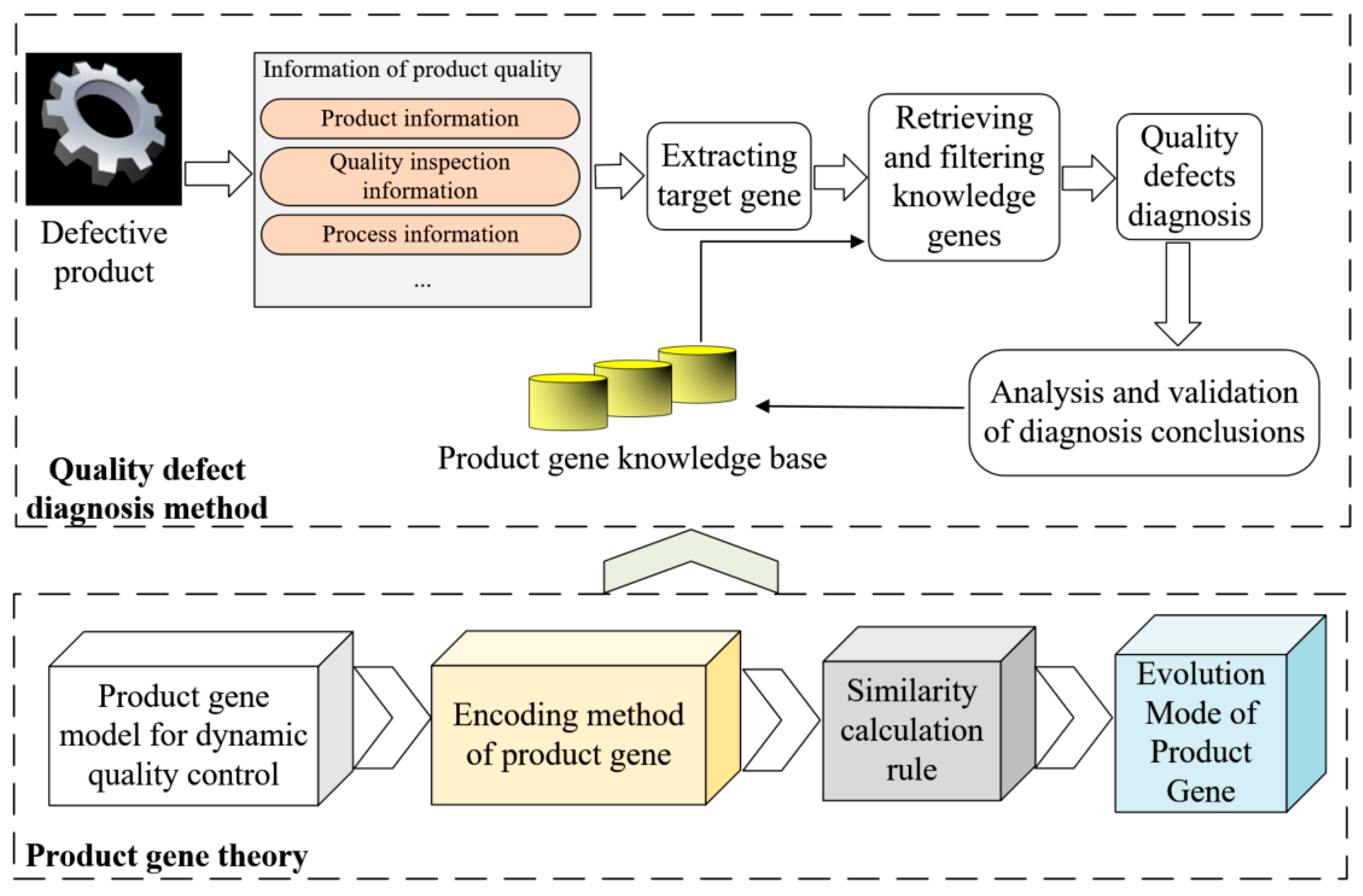
Figure 1. The research framework of the quality defects diagnosis method based on product gene theory.
Symmetry 11 00685 g001
Figure 2. Relationship between biological gene and product gene based on the processing surface.
Symmetry 11 00685 g002
Figure 3. Multi-level structure schematic diagram of the product gene.
Symmetry 11 00685 g003
Figure 4. Interrelated relation schematic diagram of product gene units.
Symmetry 11 00685 g004
Figure 5. Case data of a product gene of bearing spacer.
Symmetry 11 00685 g005
Figure 6. Evolution process of product gene.
Symmetry 11 00685 g006
Figure 7. Process of quality defects diagnosis based on product gene.
Symmetry 11 00685 g007
Figure 8. Flowchart of optimization method of weights with particle swarm optimization (PSO).
Symmetry 11 00685 g008
Figure 9. Bearing spacer of an M5018A roller press of a building material equipment enterprise.
Symmetry 11 00685 g009
Figure 10. Process card of bearing spacer of an M5018A roller press.
Symmetry 11 00685 g010
Figure 11. Evolutionary curves of the average value of the best fitnesses.
Symmetry 11 00685 g011
Table 1. Encoding method and data types of product gene.
Composition of Attribute CodeType of ValueDescription
Code of element# (values set)#(metadata set)Boolean (B)It can be described by a binary number.
Option (O)There are multiple options to be chosen and only one option can be chosen.
Discrete (D)A discrete value is a discontinuous value or it belongs to one of several discrete intervals.
Continuity (C)A continuous value is a continuous numeric value which can be computed.
String (S)A string value is described with a string which consists of one or more characters.
Table 2. Meanings of codes in GU (1).
Information SetCodeExplanation
L1-1#23#CThe unique code of GU (1) is “23” and the type of its value is continuity.
1-2#M5018A#SThe code of the equipment is “M5018A”, and the type of value is string.
1-3#1F2#SThe code of the part is “1F2” and the type of value is string.
1-4#C6#SThe code of the type of surface is “C6” and the type of value is string.
C2-1#(905.06, 905, -0.09, 0)#CThe actual diameter is 905.06 mm, the design diameter is 905 mm, the lower deviation is −0.09 mm, the upper deviation is 0 mm. The types of values are all continuity.
2-2#(3.2, 1.6)#CThe actual surface roughness is Ra3.2, the design surface roughness is Ra1.6. The types of values are both continuity.
2-3#(0.03, 0.03)#CThe actual concentricity and design concentricity are both 0.03 mm, and the type of value is continuity.
2-4#(50.2, 50, -0.3, 0.3)#CThe actual width is 50.2 mm, the design width is 50 mm, the lower deviation is -0.3 mm, the upper deviation is 0.3 mm. The types of values are all continuity.
2-5#(42, 40)#CThe actual hardness is HRC42, the design hardness is HRC40. The types of values are both continuity.
P3-11#(5, C1)#(C, S)The allowance of one side is 5 mm; the processing mode of rough turning is “C1”. The types of values are continuity and string, respectively.
3-12#(2, C2)#(C, S)The allowance of one side is 2 mm, the processing mode of semi-finish turning is “C2”. The types of values are continuity and string, respectively.
3-71#NA1#SThe mode of natural aging is “NA1” and the type of the value is string.
3-13#C3#SThe processing mode of finish turning is “C3” and the type of the value is string.
3-53#Q1#SThe mode of quenching is “Q1” and the type of the value is string.
I4-1#ZG270-500#SThe material is “ZG270-500” and the type of the value is string.
4-11#(3, C6125, 12, N1)#(C, S, C, O)The capability of worker is “3” the machine type is “C6125”, the age of machine of rough turning is 12 years. The types of values are continuity, string, continuity, and option respectively.
4-12#(3, C6125, 12, -)#(C, S, C, -)The capability of the worker is “3” the machine type is “C6125”, the age of machine of semi-finish turning is 12 years. The types of values are continuity, string, and continuity, respectively.
4-71#(16, 75, 4.2)#CThe average temperature is 16 ℃, the humidity is 75%, the time of natural aging is 4.2 hours. The types of values are all continuity.
4-13#(4, C6125, 5, N1)#(C, S, C, O)The capability of worker is “4” the machine type is “C6125” the age of the machine is 5 years, and the inspection method of finish turning is the conventional method. The types of values are continuity, string, continuity, and option, respectively.
4-53#(2, 3, 835)#CThe capability of the worker is “2” holding time is 3 minutes, the temperature of quenching is 835 ℃. The types of values are all continuity.
R5-1#(24bc, 25bc)#CThe unique codes of related surfaces are “24” and “25” respectively, and influence relationship and sequence relationship are included. The type of value is continuity.
PE6-1#sr#OThe defect is general surface roughness error and the type of value is option.
Table 3. Empirical data of quality defects and diagnosis conclusions.
Quality Defects (Fuzzy Factors)Diagnosis Conclusions (Fuzzy Classifications)
FC1FC2FC3
FF1523
FF2134
FF3212
Table 4. Knowledge genes obtained by retrieval.
IndexGU(1)GU(2)GU(3)
11-1#11#C;1-2#M5018B#S;1-3#1F2#S;1-4#C6#S;2-1#(904.99,905,-0.09,0)#C;2-2#(3.2,1.6)#C;2-3#(0.02,0.03)#C;2-4#(50.33,50,-0.15,0.3)#C;2-5#(45,42)#C;3-11#(5,C1)#(C,S);3-12#(2.1,C2)#(C,S);3-71#NA2#S;3-13#C3#S;3-53#Q2#S;4-1#ZG230-450#S;4-11#(7,C6130,7,N2)#(C,S,C,O);4-12#(7,C6130,7,-)#(C,S,C,O);4-71#(13,35,4.2)#C;4-13#(4,C6130,11,N2)#(C,S,C,O);4-53#(4,3.2,830)#C;5-1#(12,3)#C;6-1#(sr,de3)#O;7-1#(om13,mat,mt)#O1-1#12#C;1-2#M5018B#S;1-3#1F2#S;1-4#C6#S;2-1#(905.01,905,-0.09,0)#C;2-2#(755.02,755,0,0.05)#C;2-3#(1.6,1.6)#C;2-4#(50.33,50,-0.15,0.3)#C;3-11#(4.9,C11)#(C,S);3-12#(1.8,C12)#(C,S);3-71#NA2#S;3-13#C13#S;3-53#Q2#S;4-1#ZG230-450#S;4-11#(3,C6125,11,N1)#(C,S,C,O);4-12#(3,C6125,11,-)#(C,S,C,O);4-71#(13,35,4.2)#C;4-13#(4,C6125,7,N1)#(C,S,C,O);4-53#(4,3.2,830)#C;5-1#(11,3)#C1-1#3#C;1-2#M5018B#S;1-3#1F2#S;1-4#C6#S;2-1#(755.02,755,0,0.05)#C;2-2#0.8,1.6#C;2-3#(0.02,0.03)#C;2-4#(45,42)#C;2-5#(40,42)#C;3-11#(4.8,C1)#(C,S);3-12#(2.1,C2)#(C,S);3-71#NA2#S;3-13#C3#S;3-53#Q2#S;4-1#ZG230-450#S;4-11#(5,C6130,7,N1)#(C,S,C,O);4-12#(5,C6130,7,-)#(C,S,C,O);4-71#(13,35,4.2)#C;4-13#(6,C6150,8,N2)#(C,S,C,O);4-53#(4,3.2,830)#C;5-1#(11,12)#C;6-1#(de3, he1)#O;7-1#(mat,ht1)#O
21-1#13#C;1-2#M5018A#S;1-3#1F2A#S;1-4#C6#S;2-1#(799.97,800,-0.05,0)#C;2-2#(3.2,1.6)#C;2-3#(0.02,0.03)#C;2-4#(65.08,65,-0.15,0.15)#C;2-5#(42,42)#C;3-11#(4.9,C1)#(C,S);3-12#(2.1,C2)#(C,S);3-71#NA1#S;3-13#C3#S;3-53#Q1#S;4-1#ZG270-500#S;4-11#(6,C6130,10,N1)#(C,S,C,O);4-12#(6,C6130,10,N2)#(C,S,C,O);4-71#(16,15,3.9)#C;4-13#(7,C6150,11,N2)#(C,S,C,O);4-53#(3,3.2,850)#C;5-1#(14,5)#C;6-1#(sr,mc1)#O;7-1#(om11,om13,cm1, tem1)#O1-1#14#C;1-2#M5018A#S;1-3#1F2A#S;1-4#C6#S;2-1#(800.03,800,-0.05,0)#C;2-2#(650.01,650,0,0.07)#C;2-3#(3.2,3.2)#C;2-4#(65.08,65,-0.15,0.15)#C;3-11#(5.2,C11)#(C,S);3-12#(1.8,C12)#(C,S);3-71#NA1#S;3-13#C13#S;3-53#Q1#S;4-1#ZG270-500#S;4-11#(2,C6130,7,N1)#(C,S,C,O);4-12#(2,C6130,7,N1)#(C,S,C,O);4-71#(16,15,3.9)#C;4-13#(4,C6150,8,N1)#(C,S,C,O);4-53#(3,3.2,850)#C;5-1#(13,5)#C1-1#5#C;1-2#M5018A#S;1-3#1F2A#S;1-4#C6#S;2-1#(650.01,650,0,0.07)#C;2-2#0.8,1.6#C;2-3#(0.02,0.01)#C;2-4#(45,40)#C;2-5#(40,40)#C;3-11#(4.9,C1)#(C,S);3-12#(2,C2)#(C,S);3-71#NA1#S;3-13#C3#S;3-53#Q1#S;4-1#ZG270-500#S;4-11#(5,C6125,8,N1)#(C,S,C,O);4-12#(5,C6125,8,N2)#(C,S,C,O);4-71#(16,15,3.9)#C;4-13#(7,C6150,3,N1)#(C,S,C,O);4-53#(3,3.2,850)#C;5-1#(13,14)#C;6-1#(mc1,ce1)#O;7-1#(pw13,tem1)#O
31-1#15#C;1-2#M5018A#S;1-3#1F2#S;1-4#C6#S;2-1#(905.03,905,-0.056,0)#C;2-2#(3.2,3.2)#C;2-3#(0.02,0.01)#C;2-4#(65.15,65,-0.15,0.3)#C;2-5#(42,40)#C;3-11#(5.2,C1)#(C,S);3-12#(2.1,C2)#(C,S);3-71#NA1#S;3-13#C3#S;3-53#Q2#S;4-1#ZG230-450#S;4-11#(7,C6150,5,N2)#(C,S,C,O);4-12#(7,C6150,5,N2)#(C,S,C,O);4-71#(13,35,4.2)#C;4-13#(4,C6150,3,N2)#(C,S,C,O);4-53#(7,3.5,840)#C;5-1#(16,6)#C;6-1#(ce1,de1)#O;7-1#(om13,pw13)#O1-1#16#C;1-2#M5018A#S;1-3#1F2#S;1-4#C6#S;2-1#(905.10,905,-0.056,0)#C;2-2#(755.08,755,0,0.08)#C;2-3#(0.8,3.2)#C;2-4#(65.15,65,-0.15,0.3)#C;3-11#(5,C11)#(C,S);3-12#(1.8,C12)#(C,S);3-71#NA1#S;3-13#C13#S;3-53#Q2#S;4-1#ZG230-450#S;4-11#(4,C6130,3,N2)#(C,S,C,O);4-12#(4,C6130,3,N1)#(C,S,C,O);4-71#(13,35,4.2)#C;4-13#(4,C6150,3,N2)#(C,S,C,O);4-53#(7,3.5,840)#C;5-1#(15,6)#C1-1#6#C;1-2#M5018A#S;1-3#1F2#S;1-4#C6#S;2-1#(755.08,755,0,0.08)#C;2-2#3.2,3.2#C;2-3#(0.03,0.02)#C;2-4#(44,42)#C;2-5#(45,40)#C;3-11#(5.1,C1)#(C,S);3-12#(2,C2)#(C,S);3-71#NA1#S;3-13#C3#S;3-53#Q2#S;4-1#ZG230-450#S;4-11#(4,C6150,8,N2)#(C,S,C,O);4-12#(4,C6150,8,-)#(C,S,C,O);4-71#(13,35,4.2)#C;4-13#(3,C6125,5,N1)#(C,S,C,O);4-53#(7,3.5,840)#C;5-1#(15,16)#C;6-1#(ce1)#O;7-1#(mt,pw13)#O
4
Table 5. Meanings of abbreviations of quality defects and causes.
Element CodeAbbreviationExplanation
6-1srIt indicates that the surface roughness is too large.
mc1It indicates the existence of microcracks on the surface.
ce1It indicates that the concentricity error is too large.
de1It indicates that the diameter error is greater than the upper deviation.
de2It indicates that the diameter error is less than the lower deviation.
de3It indicates that the width error is greater than the upper deviation.
de4It indicates that the width error is less than the lower deviation.
bhIt indicates the existence of blowholes on the surface.
impIt indicates the existence of impurities on the surface.
he1It indicates that the surface hardness is lower than its design value.
7-1om11It indicates that the machine of rough turning or semi-finish turning is too old.
om13It indicates that the machine of finish turning is too old.
matIt indicates that the material is inappropriate or unqualified
mtIt indicates that the error of measuring tools is too large.
pw11It indicates that the worker who carries out rough turning is not skilled enough.
pw13It indicates that the worker who carries out finish turning is not skilled enough.
pw53It indicates that the worker who carries out quenching is not skilled enough.
cm1It indicates that the structure of casting mold is unreasonable.
cm2It indicates that the casting mold has not been cleaned up.
ht1It indicates that the holding time of quenching is too short.
ht2It indicates that the holding time of quenching is too long.
tem1It means that the temperature of quenching is too high.
tem2It means that the temperature of quenching is too low.
Table 6. Relevant knowledge genes filtered by direct similarity.
IndexGU(1)GU(2)GU(3)
11-1#11#C;1-2#M5018B#S;1-3#1F2#S;1-4#C6#S;2-1#(904.99,905,-0.09,0)#C;2-2#(3.2,1.6)#C;2-3#(0.02,0.03)#C;2-4#(50.33,50,-0.15,0.3)#C;2-5#(45,42)#C;3-11#(5,C1)#(C,S);3-12#(2.1,C2)#(C,S);3-71#NA2#S;3-13#C3#S;3-53#Q2#S;4-1#ZG230-450#S;4-11#(7,C6130,7,N2)#(C,S,C,O);4-12#(7,C6130,7,-)#(C,S,C,O);4-71#(13,35,4.2)#C;4-13#(4,C6130,11,N2)#(C,S,C,O);4-53#(4,3.2,830)#C;5-1#(12,3)#C;6-1#(sr,de3)#O;7-1#(om13,mat,mt)#O1-1#12#C;1-2#M5018B#S;1-3#1F2#S;1-4#C6#S;2-1#(905.01,905,-0.09,0)#C;2-2#(755.02,755,0,0.05)#C;2-3#(1.6,1.6)#C;2-4#(50.33,50,-0.15,0.3)#C;3-11#(4.9,C11)#(C,S);3-12#(1.8,C12)#(C,S);3-71#NA2#S;3-13#C13#S;3-53#Q2#S;4-1#ZG230-450#S;4-11#(3,C6125,11,N1)#(C,S,C,O);4-12#(3,C6125,11,-)#(C,S,C,O);4-71#(13,35,4.2)#C;4-13#(4,C6125,7,N1)#(C,S,C,O);4-53#(4,3.2,830)#C;5-1#(11,3)#C1-1#3#C;1-2#M5018B#S;1-3#1F2#S;1-4#C6#S;2-1#(755.02,755,0,0.05)#C;2-2#0.8,1.6#C;2-3#(0.02,0.03)#C;2-4#(45,42)#C;2-5#(40,42)#C;3-11#(4.8,C1)#(C,S);3-12#(2.1,C2)#(C,S);3-71#NA2#S;3-13#C3#S;3-53#Q2#S;4-1#ZG230-450#S;4-11#(5,C6130,7,N1)#(C,S,C,O);4-12#(5,C6130,7,-)#(C,S,C,O);4-71#(13,35,4.2)#C;4-13#(6,C6150,8,N2)#(C,S,C,O);4-53#(4,3.2,830)#C;5-1#(11,12)#C;6-1#(de3, he1)#O;7-1#(mat,ht1)#O
21-1#13#C;1-2#M5018A#S;1-3#1F2A#S;1-4#C6#S;2-1#(799.97,800,-0.05,0)#C;2-2#(3.2,1.6)#C;2-3#(0.02,0.03)#C;2-4#(65.08,65,-0.15,0.15)#C;2-5#(42,42)#C;3-11#(4.9,C1)#(C,S);3-12#(2.1,C2)#(C,S);3-71#NA1#S;3-13#C3#S;3-53#Q1#S;4-1#ZG270-500#S;4-11#(6,C6130,10,N1)#(C,S,C,O);4-12#(6,C6130,10,N2)#(C,S,C,O);4-71#(16,15,3.9)#C;4-13#(7,C6150,11,N2)#(C,S,C,O);4-53#(3,3.2,850)#C;5-1#(14,5)#C;6-1#(sr,mc1)#O;7-1#(om11,om13,cm1,tem1)#O1-1#14#C;1-2#M5018A#S;1-3#1F2A#S;1-4#C6#S;2-1#(800.03,800,-0.05,0)#C;2-2#(650.01,650,0,0.07)#C;2-3#(3.2,3.2)#C;2-4#(65.08,65,-0.15,0.15)#C;3-11#(5.2,C11)#(C,S);3-12#(1.8,C12)#(C,S);3-71#NA1#S;3-13#C13#S;3-53#Q1#S;4-1#ZG270-500#S;4-11#(2,C6130,7,N1)#(C,S,C,O);4-12#(2,C6130,7,N1)#(C,S,C,O);4-71#(16,15,3.9)#C;4-13#(4,C6150,8,N1)#(C,S,C,O);4-53#(3,3.2,850)#C;5-1#(13,5)#C1-1#5#C;1-2#M5018A#S;1-3#1F2A#S;1-4#C6#S;2-1#(650.01,650,0,0.07)#C;2-2#0.8,1.6#C;2-3#(0.02,0.01)#C;2-4#(45,40)#C;2-5#(40,40)#C;3-11#(4.9,C1)#(C,S);3-12#(2,C2)#(C,S);3-71#NA1#S;3-13#C3#S;3-53#Q1#S;4-1#ZG270-500#S;4-11#(5,C6125,8,N1)#(C,S,C,O);4-12#(5,C6125,8,N2)#(C,S,C,O);4-71#(16,15,3.9)#C;4-13#(7,C6150,3,N1)#(C,S,C,O);4-53#(3,3.2,850)#C;5-1#(13,14)#C;6-1#(mc1,ce1)#O;7-1#(pw13,tem1)#O
51-1#19#C;1-2#SLC301#S;1-3#1F2R#S;1-4#C6#S;2-1#(774.99,775,-0.08,0)#C;2-2#(0.8,1.6)#C;2-3#(0.03,0.03)#C;2-4#(69.81,70,-0.15,0.15)#C;2-5#(43,40)#C;3-11#(5,C1)#(C,S);3-12#(1.8,C2)#(C,S);3-71#NA1#S;3-13#C3#S;3-53#Q1#S;4-1#ZG230-450#S;4-11#(3,C6150,8,N1)#(C,S,C,O);4-12#(3,C6150,8,N2)#(C,S,C,O);4-71#(16,50,4.2)#C;4-13#(2,C6130,3,N1)#(C,S,C,O);4-53#(7,3.8,850)#C;5-1#(21,9)#C;6-1#(sr,mc1,de4)#O;7-1#(mt,pw11,pw13,cm1,tem1)#O1-1#21#C;1-2#SLC301#S;1-3#1F2R#S;1-4#C6#S;2-1#(775.02,775,-0.08,0)#C;2-2#(625.04,625,0,0.44)#C;2-3#(1.6,1.6)#C;2-4#(69.91,70,-0.15,0.15)#C;3-11#(5.2,C11)#(C,S);3-12#(2.1,C12)#(C,S);3-71#NA1#S;3-13#C13#S;3-53#Q1#S;4-1#ZG230-450#S;4-11#(3,C6130,8,N2)#(C,S,C,O);4-12#(3,C6130,8,N2)#(C,S,C,O);4-71#(16,50,4.2)#C;4-13#(6,C6130,11,N2)#(C,S,C,O);4-53#(7,3.8,850)#C;5-1#(19,9)#C;6-1#(sr,mc1)#O;7-1#(om13,mt,pw11,cm1,tem1)#O1-1#9#C;1-2#SLC301#S;1-3#1F2R#S;1-4#C6#S;2-1#(625.04,625,0,0.44)#C;2-2#3.2,3.2#C;2-3#(0.02,0.02)#C;2-4#(42,40)#C;2-5#(44,42)#C;3-11#(5.1,C1)#(C,S);3-12#(2.2,C2)#(C,S);3-71#NA1#S;3-13#C3#S;3-53#Q1#S;4-1#ZG230-450#S;4-11#(6,C6125,10,N1)#(C,S,C,O);4-12#(6,C6125,10,N1)#(C,S,C,O);4-71#(16,50,4.2)#C;4-13#(5,C6150,10,N2)#(C,S,C,O);4-53#(7,3.8,850)#C;5-1#(19,21)#C;6-1#(sr,mc1)#O;7-1#(mt,cm1,ht2,tem1)#O
111-1#66#C;1-2#TRMC202#S;1-3#1F2#S;1-4#C6#S;2-1#(904.99,905,-0.056,0)#C;2-2#(3.2,1.6)#C;2-3#(0.02,0.05)#C;2-4#(64.83,65,-0.15,0.3)#C;2-5#(41,40)#C;3-11#(4.8,C1)#(C,S);3-12#(2.1,C2)#(C,S);3-71#NA1#S;3-13#C3#S;3-53#Q2#S;4-1#ZG230-450#S;4-11#(5,C6125,7,N1)#(C,S,C,O);4-12#(5,C6125,7,N2)#(C,S,C,O);4-71#(21,75,4.2)#C;4-13#(6,C6125,8,N2)#(C,S,C,O);4-53#(7,3.2,850)#C;5-1#(62,34)#C;6-1#(sr,de4)#O;7-1#(mat,mt,cm1)#O1-1#62#C;1-2#TRMC202#S;1-3#1F2#S;1-4#C6#S;2-1#(905.01,905,-0.056,0)#C;2-2#(755.02,755,0,0.08)#C;2-3#(3.2,1.6)#C;2-4#(65.13,65,-0.15,0.3)#C;3-11#(5.2,C11)#(C,S);3-12#(2.2,C12)#(C,S);3-71#NA1#S;3-13#C13#S;3-53#Q2#S;4-1#ZG230-450#S;4-11#(5,C6150,7,N2)#(C,S,C,O);4-12#(5,C6150,7,-)#(C,S,C,O);4-71#(21,75,4.2)#C;4-13#(6,C6125,11,N1)#(C,S,C,O);4-53#(7,3.2,850)#C;5-1#(66,34)#C;6-1#(sr)#O;7-1#(om13)#O1-1#34#C;1-2#TRMC202#S;1-3#1F2#S;1-4#C6#S;2-1#(755.02,755,0,0.08)#C;2-2#3.2,1.6#C;2-3#(0.03,0.03)#C;2-4#(44,42)#C;2-5#(42,42)#C;3-11#(5,C1)#(C,S);3-12#(2.2,C2)#(C,S);3-71#NA1#S;3-13#C3#S;3-53#Q2#S;4-1#ZG230-450#S;4-11#(6,C6125,7,N1)#(C,S,C,O);4-12#(6,C6125,7,N2)#(C,S,C,O);4-71#(21,75,4.2)#C;4-13#(5,C6150,3,N1)#(C,S,C,O);4-53#(7,3.2,850)#C;5-1#(66,62)#C;6-1#(sr)#O;7-1#(mt)#O
141-1#71#C;1-2#M5018R#S;1-3#1F2R#S;1-4#C6#S;2-1#(775.02,775,-0.05,0)#C;2-2#(3.2,1.6)#C;2-3#(0.01,0.02)#C;2-4#(69.95,70,-0.15,0.3)#C;2-5#(40,42)#C;3-11#(5.1,C1)#(C,S);3-12#(2,C2)#(C,S);3-71#NA2#S;3-13#C3#S;3-53#Q1#S;4-1#ZG270-500#S;4-11#(5,C6130,8,N2)#(C,S,C,O);4-12#(5,C6130,8,N1)#(C,S,C,O);4-71#(21,75,3.9)#C;4-13#(6,C6150,3,N2)#(C,S,C,O);4-53#(7,3.8,850)#C;5-1#(73,45)#C;6-1#(sr,de1,he1)#O;7-1#(mt,tem1)#O1-1#73#C;1-2#M5018R#S;1-3#1F2R#S;1-4#C6#S;2-1#(775.08,775,-0.05,0)#C;2-2#(625.05,625,0,0.07)#C;2-3#(1.6,1.6)#C;2-4#(69.95,70,-0.15,0.3)#C;3-11#(4.8,C11)#(C,S);3-12#(2.2,C12)#(C,S);3-71#NA2#S;3-13#C13#S;3-53#Q1#S;4-1#ZG270-500#S;4-11#(7,C6150,10,N2)#(C,S,C,O);4-12#(7,C6150,10,-)#(C,S,C,O);4-71#(21,75,3.9)#C;4-13#(4,C6125,8,N2)#(C,S,C,O);4-53#(7,3.8,850)#C;5-1#(71,45)#C1-1#45#C;1-2#M5018R#S;1-3#1F2R#S;1-4#C6#S;2-1#(625.05,625,0,0.07)#C;2-2#3.2,1.6#C;2-3#(0.02,0.03)#C;2-4#(41,40)#C;2-5#(45,40)#C;3-11#(5.1,C1)#(C,S);3-12#(2.1,C2)#(C,S);3-71#NA2#S;3-13#C3#S;3-53#Q1#S;4-1#ZG270-500#S;4-11#(3,C6125,11,N2)#(C,S,C,O);4-12#(3,C6125,11,N1)#(C,S,C,O);4-71#(21,75,3.9)#C;4-13#(5,C6130,3,N1)#(C,S,C,O);4-53#(7,3.8,850)#C;5-1#(71,73)#C;6-1#(sr)#O;7-1#(om11,pw11)#O
151-1#83#C;1-2#TRMC202#S;1-3#1F2#S;1-4#C6#S;2-1#(904.91,905,-0.056,0)#C;2-2#(1.6,1.6)#C;2-3#(0.02,0.02)#C;2-4#(49.92,50,-0.15,0.15)#C;2-5#(43,40)#C;3-11#(5,C1)#(C,S);3-12#(2,C2)#(C,S);3-71#NA1#S;3-13#C3#S;3-53#Q1#S;4-1#ZG270-500#S;4-11#(2,C6130,3,N1)#(C,S,C,O);4-12#(2,C6130,3,N2)#(C,S,C,O);4-71#(13,15,4.7)#C;4-13#(5,C6150,5,N1)#(C,S,C,O);4-53#(3,3.2,830)#C;5-1#(77,46)#C;6-1#(de2)#O;7-1#(pw11,tem2)#O1-1#77#C;1-2#TRMC202#S;1-3#1F2#S;1-4#C6#S;2-1#(905.10,905,-0.056,0)#C;2-2#(755.08,755,0,0.08)#C;2-3#(0.8,3.2)#C;2-4#(49.92,50,-0.15,0.15)#C;3-11#(5.2,C11)#(C,S);3-12#(2,C12)#(C,S);3-71#NA1#S;3-13#C13#S;3-53#Q1#S;4-1#ZG270-500#S;4-11#(7,C6130,5,N1)#(C,S,C,O);4-12#(7,C6130,5,N2)#(C,S,C,O);4-71#(13,15,4.7)#C;4-13#(5,C6125,8,N1)#(C,S,C,O);4-53#(3,3.2,830)#C;5-1#(83,46)#C1-1#46#C;1-2#TRMC202#S;1-3#1F2#S;1-4#C6#S;2-1#(755.09,755,0,0.08)#C;2-2#3.2,1.6#C;2-3#(0.03,0.01)#C;2-4#(44,42)#C;2-5#(44,40)#C;3-11#(5,C1)#(C,S);3-12#(2.2,C2)#(C,S);3-71#NA1#S;3-13#C3#S;3-53#Q1#S;4-1#ZG270-500#S;4-11#(2,C6125,5,N2)#(C,S,C,O);4-12#(2,C6125,5,-)#(C,S,C,O);4-71#(13,15,4.7)#C;4-13#(6,C6130,11,N1)#(C,S,C,O);4-53#(3,3.2,830)#C;5-1#(83,77)#C;6-1#(sr,ce1,de1)#O;7-1#(om13,pw11,tem2)#O
161-1#85#C;1-2#M5018R#S;1-3#1F2A#S;1-4#C6#S;2-1#(799.97,800,-0.08,0)#C;2-2#(1.6,1.6)#C;2-3#(0.03,0.03)#C;2-4#(50.21,50,-0.3,0.3)#C;2-5#(43,42)#C;3-11#(5.1,C1)#(C,S);3-12#(2.2,C2)#(C,S);3-71#NA1#S;3-13#C3#S;3-53#Q2#S;4-1#ZG270-500#S;4-11#(2,C6150,3,N1)#(C,S,C,O);4-12#(2,C6150,3,N1)#(C,S,C,O);4-71#(13,35,5.5)#C;4-13#(3,C6150,10,N2)#(C,S,C,O);4-53#(7,3.2,835)#C;5-1#(80,48)#C;6-1#(bh,imp)#O;7-1#(pw11,cm2)#O1-1#80#C;1-2#M5018R#S;1-3#1F2A#S;1-4#C6#S;2-1#(800.03,800,-0.08,0)#C;2-2#(650.01,650,0,0.44)#C;2-3#(3.2,1.6)#C;2-4#(50.21,50,-0.3,0.3)#C;3-11#(4.9,C11)#(C,S);3-12#(2.2,C12)#(C,S);3-71#NA1#S;3-13#C13#S;3-53#Q2#S;4-1#ZG270-500#S;4-11#(3,C6150,3,N2)#(C,S,C,O);4-12#(3,C6150,3,N1)#(C,S,C,O);4-71#(13,35,5.5)#C;4-13#(5,C6150,3,N1)#(C,S,C,O);4-53#(7,3.2,835)#C;5-1#(85,48)#C;6-1#(sr,imp)#O;7-1#(mt,pw11,cm2)#O1-1#48#C;1-2#M5018R#S;1-3#1F2A#S;1-4#C6#S;2-1#(650.01,650,0,0.44)#C;2-2#3.2,1.6#C;2-3#(0.02,0.05)#C;2-4#(42,42)#C;2-5#(43,42)#C;3-11#(4.8,C1)#(C,S);3-12#(2.2,C2)#(C,S);3-71#NA1#S;3-13#C3#S;3-53#Q2#S;4-1#ZG270-500#S;4-11#(7,C6130,8,N1)#(C,S,C,O);4-12#(7,C6130,8,N1)#(C,S,C,O);4-71#(13,35,5.5)#C;4-13#(3,C6125,5,N2)#(C,S,C,O);4-53#(7,3.2,835)#C;5-1#(85,80)#C;6-1#(sr,bh,imp)#O;7-1#(pw13,cm2)#O
171-1#86#C;1-2#TRM113#S;1-3#1F2A#S;1-4#C6#S;2-1#(799,98,800,-0.08,0)#C;2-2#(3.2,1.6)#C;2-3#(0.02,0.02)#C;2-4#(65.17,65,-0.3,0.3)#C;2-5#(43,40)#C;3-11#(4.8,C1)#(C,S);3-12#(1.8,C2)#(C,S);3-71#NA2#S;3-13#C3#S;3-53#Q1#S;4-1#ZG230-450#S;4-11#(7,C6130,5,N1)#(C,S,C,O);4-12#(7,C6130,5,N2)#(C,S,C,O);4-71#(16,75,4.2)#C;4-13#(5,C6125,7,N1)#(C,S,C,O);4-53#(7,3,840)#C;5-1#(81,51)#C;6-1#(sr,imp)#O;7-1#(cm2,ht1)#O1-1#81#C;1-2#TRM113#S;1-3#1F2A#S;1-4#C6#S;2-1#(800.02,800,-0.08,0)#C;2-2#(650.03,650,0,0.44)#C;2-3#(3.2,1.6)#C;2-4#(65.17,65,-0.3,0.3)#C;3-11#(4.9,C11)#(C,S);3-12#(1.9,C12)#(C,S);3-71#NA2#S;3-13#C13#S;3-53#Q1#S;4-1#ZG230-450#S;4-11#(6,C6150,7,N1)#(C,S,C,O);4-12#(6,C6150,7,-)#(C,S,C,O);4-71#(16,75,4.2)#C;4-13#(3,C6150,5,N1)#(C,S,C,O);4-53#(7,3,840)#C;5-1#(86,51)#C;6-1#(sr,imp,he1)#O;7-1#(cm2,ht1)#O1-1#51#C;1-2#TRM113#S;1-3#1F2A#S;1-4#C6#S;2-1#(650.03,650,0,0.44)#C;2-2#0.8,3.2#C;2-3#(0.02,0.02)#C;2-4#(40,42)#C;2-5#(41,40)#C;3-11#(5.2,C1)#(C,S);3-12#(1.8,C2)#(C,S);3-71#NA2#S;3-13#C3#S;3-53#Q1#S;4-1#ZG230-450#S;4-11#(6,C6150,10,N1)#(C,S,C,O);4-12#(6,C6150,10,N1)#(C,S,C,O);4-71#(16,75,4.2)#C;4-13#(4,C6150,10,N1)#(C,S,C,O);4-53#(7,3,840)#C;5-1#(86,81)#C;6-1#(imp)#O;7-1#(om11,om13,cm2)#O
191-1#90#C;1-2#M5018B#S;1-3#1F2#S;1-4#C6#S;2-1#(904.99,905,-0.09,0)#C;2-2#(0.8,3.2)#C;2-3#(0.02,0.03)#C;2-4#(64.95,65,-0.15,0.3)#C;2-5#(45,40)#C;3-11#(4.9,C1)#(C,S);3-12#(1.9,C2)#(C,S);3-71#NA2#S;3-13#C3#S;3-53#Q1#S;4-1#ZG230-450#S;4-11#(2,C6130,8,N2)#(C,S,C,O);4-12#(2,C6130,8,-)#(C,S,C,O);4-71#(21,35,4.2)#C;4-13#(6,C6130,10,N2)#(C,S,C,O);4-53#(2,3.2,835)#C;5-1#(91,56)#C;6-1#(mc1)#O;7-1#(pw11,cm1)#O1-1#91#C;1-2#M5018B#S;1-3#1F2#S;1-4#C6#S;2-1#(905.01,905,-0.09,0)#C;2-2#(755.02,755,0,0.05)#C;2-3#(0.8,3.2)#C;2-4#(64.82,65,-0.15,0.3)#C;3-11#(4.9,C11)#(C,S);3-12#(1.9,C12)#(C,S);3-71#NA2#S;3-13#C13#S;3-53#Q1#S;4-1#ZG230-450#S;4-11#(5,C6130,7,N1)#(C,S,C,O);4-12#(5,C6130,7,N1)#(C,S,C,O);4-71#(21,35,4.2)#C;4-13#(7,C6150,11,N1)#(C,S,C,O);4-53#(2,3.2,835)#C;5-1#(90,56)#C;6-1#(mc1)#O;7-1#(om13,cm1)#O1-1#56#C;1-2#M5018B#S;1-3#1F2#S;1-4#C6#S;2-1#(755.02,755,0,0.05)#C;2-2#3.2,1.6#C;2-3#(0.03,0.01)#C;2-4#(45,42)#C;2-5#(42,42)#C;3-11#(5.2,C1)#(C,S);3-12#(1.8,C2)#(C,S);3-71#NA2#S;3-13#C3#S;3-53#Q1#S;4-1#ZG230-450#S;4-11#(6,C6125,5,N2)#(C,S,C,O);4-12#(6,C6125,5,N2)#(C,S,C,O);4-71#(21,35,4.2)#C;4-13#(5,C6130,11,N1)#(C,S,C,O);4-53#(2,3.2,835)#C;5-1#(90,91)#C;6-1#(sr,mc1,ce1,de4)#O;7-1#(om13,mat,mt,cm1)#O
211-1#94#C;1-2#M5018B#S;1-3#1F2R#S;1-4#C6#S;2-1#(774.93,775,-0.05,0)#C;2-2#(0.8,3.2)#C;2-3#(0.03,0.02)#C;2-4#(65.15,65,-0.15,0.15)#C;2-5#(41,40)#C;3-11#(5,C1)#(C,S);3-12#(2.1,C2)#(C,S);3-71#NA1#S;3-13#C3#S;3-53#Q1#S;4-1#ZG270-500#S;4-11#(3,C6125,5,N2)#(C,S,C,O);4-12#(3,C6125,5,-)#(C,S,C,O);4-71#(26,15,4.5)#C;4-13#(3,C6125,3,N2)#(C,S,C,O);4-53#(2,3.8,840)#C;5-1#(95,60)#C;6-1#(ce1,de2)#O;7-1#(pw11,pw13)#O1-1#95#C;1-2#M5018B#S;1-3#1F2R#S;1-4#C6#S;2-1#(775.08,775,-0.05,0)#C;2-2#(625.05,625,0,0.07)#C;2-3#(1.6,1.6)#C;2-4#(64.80,65,-0.15,0.15)#C;3-11#(4.8,C11)#(C,S);3-12#(2.2,C12)#(C,S);3-71#NA1#S;3-13#C13#S;3-53#Q1#S;4-1#ZG270-500#S;4-11#(5,C6150,5,N2)#(C,S,C,O);4-12#(5,C6150,5,N2)#(C,S,C,O);4-71#(26,15,4.5)#C;4-13#(2,C6125,10,N2)#(C,S,C,O);4-53#(2,3.8,840)#C;5-1#(94,60)#C1-1#60#C;1-2#M5018B#S;1-3#1F2R#S;1-4#C6#S;2-1#(625.05,625,0,0.07)#C;2-2#1.6,1.6#C;2-3#(0.02,0.02)#C;2-4#(41,40)#C;2-5#(42,42)#C;3-11#(5,C1)#(C,S);3-12#(1.9,C2)#(C,S);3-71#NA1#S;3-13#C3#S;3-53#Q1#S;4-1#ZG270-500#S;4-11#(3,C6150,10,N2)#(C,S,C,O);4-12#(3,C6150,10,-)#(C,S,C,O);4-71#(26,15,4.5)#C;4-13#(6,C6125,5,N1)#(C,S,C,O);4-53#(2,3.8,840)#C;5-1#(94,95)#C;6-1#(de4)#O;7-1#(om11,pw11)#O
251-1#106#C;1-2#M5018R#S;1-3#1F2#S;1-4#C6#S;2-1#(904.99,905,-0.09,0)#C;2-2#(0.8,1.6)#C;2-3#(0.02,0.05)#C;2-4#(50.20,50,-0.15,0.15)#C;2-5#(40,40)#C;3-11#(4.8,C1)#(C,S);3-12#(2.2,C2)#(C,S);3-71#NA1#S;3-13#C3#S;3-53#Q2#S;4-1#ZG230-450#S;4-11#(6,C6125,5,N1)#(C,S,C,O);4-12#(6,C6125,5,N1)#(C,S,C,O);4-71#(21,50,3.9)#C;4-13#(2,C6125,11,N2)#(C,S,C,O);4-53#(5,3,850)#C;5-1#(107,72)#C;6-1#(de3,bh)#O;7-1#(om13,pw13,tem1)#O1-1#107#C;1-2#M5018R#S;1-3#1F2#S;1-4#C6#S;2-1#(905.01,905,-0.09,0)#C;2-2#(755.02,755,0,0.05)#C;2-3#(1.6,3.2)#C;2-4#(50.20,50,-0.15,0.15)#C;3-11#(4.9,C11)#(C,S);3-12#(2.2,C12)#(C,S);3-71#NA1#S;3-13#C13#S;3-53#Q2#S;4-1#ZG230-450#S;4-11#(5,C6150,10,N1)#(C,S,C,O);4-12#(5,C6150,10,-)#(C,S,C,O);4-71#(21,50,3.9)#C;4-13#(4,C6150,11,N1)#(C,S,C,O);4-53#(5,3,850)#C;5-1#(106,72)#C;6-1#(bh,he1)#O;7-1#(om11,om13,tem1)#O1-1#72#C;1-2#M5018R#S;1-3#1F2#S;1-4#C6#S;2-1#(755.02,755,0,0.05)#C;2-2#3.2,1.6#C;2-3#(0.02,0.05)#C;2-4#(40,42)#C;2-5#(45,42)#C;3-11#(5.1,C1)#(C,S);3-12#(2,C2)#(C,S);3-71#NA1#S;3-13#C3#S;3-53#Q2#S;4-1#ZG230-450#S;4-11#(2,C6150,10,N1)#(C,S,C,O);4-12#(2,C6150,10,-)#(C,S,C,O);4-71#(21,50,3.9)#C;4-13#(6,C6130,10,N1)#(C,S,C,O);4-53#(5,3,850)#C;5-1#(106,107)#C;6-1#(sr,de3,bh)#O;7-1#(om11,om13,pw11,tem1)#O
261-1#109#C;1-2#M5018R#S;1-3#1F2R#S;1-4#C6#S;2-1#(774.98,775,-0.08,0)#C;2-2#(1.6,3.2)#C;2-3#(0.02,0.05)#C;2-4#(50.10,50,-0.3,0.15)#C;2-5#(44,42)#C;3-11#(5,C1)#(C,S);3-12#(1.9,C2)#(C,S);3-71#NA1#S;3-13#C3#S;3-53#Q1#S;4-1#ZG270-500#S;4-11#(7,C6130,8,N2)#(C,S,C,O);4-12#(7,C6130,8,N2)#(C,S,C,O);4-71#(13,75,5.5)#C;4-13#(7,C6150,5,N2)#(C,S,C,O);4-53#(7,3.8,840)#C;5-1#(108,75)#C1-1#108#C;1-2#M5018R#S;1-3#1F2R#S;1-4#C6#S;2-1#(775.02,775,-0.08,0)#C;2-2#(625.04,625,0,0.44)#C;2-3#(0.8,3.2)#C;2-4#(50.10,50,-0.3,0.15)#C;3-11#(5.1,C11)#(C,S);3-12#(2.2,C12)#(C,S);3-71#NA1#S;3-13#C13#S;3-53#Q1#S;4-1#ZG270-500#S;4-11#(7,C6130,8,N1)#(C,S,C,O);4-12#(7,C6130,8,N2)#(C,S,C,O);4-71#(13,75,5.5)#C;4-13#(6,C6125,5,N2)#(C,S,C,O);4-53#(7,3.8,840)#C;5-1#(109,75)#C1-1#75#C;1-2#M5018R#S;1-3#1F2R#S;1-4#C6#S;2-1#(625.04,625,0,0.44)#C;2-2#1.6,1.6#C;2-3#(0.02,0.02)#C;2-4#(42,42)#C;2-5#(40,42)#C;3-11#(4.9,C1)#(C,S);3-12#(1.9,C2)#(C,S);3-71#NA1#S;3-13#C3#S;3-53#Q1#S;4-1#ZG270-500#S;4-11#(2,C6125,11,N2)#(C,S,C,O);4-12#(2,C6125,11,-)#(C,S,C,O);4-71#(13,75,5.5)#C;4-13#(6,C6130,10,N1)#(C,S,C,O);4-53#(7,3.8,840)#C;5-1#(109,108)#C;6-1#(he1)#O;7-1#(mat)#O
271-1#110#C;1-2#M5018B#S;1-3#1F2A#S;1-4#C6#S;2-1#(799.98,800,-0.05,0)#C;2-2#(0.8,3.2)#C;2-3#(0.03,0.03)#C;2-4#(65.08,65,-0.15,0.15)#C;2-5#(42,40)#C;3-11#(5,C1)#(C,S);3-12#(2,C2)#(C,S);3-71#NA2#S;3-13#C3#S;3-53#Q1#S;4-1#ZG230-450#S;4-11#(5,C6150,5,N2)#(C,S,C,O);4-12#(5,C6150,5,N1)#(C,S,C,O);4-71#(26,50,4.2)#C;4-13#(2,C6130,8,N2)#(C,S,C,O);4-53#(4,3.8,835)#C;5-1#(111,78)#C;6-1#(mc1)#O;7-1#(mat,cm1)#O1-1#111#C;1-2#M5018B#S;1-3#1F2A#S;1-4#C6#S;2-1#(800.02,800,-0.05,0)#C;2-2#(650.03,650,0,0.07)#C;2-3#(1.6,3.2)#C;2-4#(65.08,65,-0.15,0.15)#C;3-11#(4.8,C11)#(C,S);3-12#(1.8,C12)#(C,S);3-71#NA2#S;3-13#C13#S;3-53#Q1#S;4-1#ZG230-450#S;4-11#(6,C6125,5,N2)#(C,S,C,O);4-12#(6,C6125,5,-)#(C,S,C,O);4-71#(26,50,4.2)#C;4-13#(4,C6130,7,N1)#(C,S,C,O);4-53#(4,3.8,835)#C;5-1#(110,78)#C;6-1#(mc1)#O;7-1#(mat,cm1)#O1-1#78#C;1-2#M5018B#S;1-3#1F2A#S;1-4#C6#S;2-1#(650.03,650,0,0.07)#C;2-2#1.6,3.2#C;2-3#(0.02,0.03)#C;2-4#(43,42)#C;2-5#(45,42)#C;3-11#(5.1,C1)#(C,S);3-12#(2.1,C2)#(C,S);3-71#NA2#S;3-13#C3#S;3-53#Q1#S;4-1#ZG230-450#S;4-11#(3,C6125,3,N1)#(C,S,C,O);4-12#(3,C6125,3,N2)#(C,S,C,O);4-71#(26,50,4.2)#C;4-13#(4,C6150,10,N2)#(C,S,C,O);4-53#(4,3.8,835)#C;5-1#(110,111)#C;6-1#(mc1)#O;7-1#(mat,cm1)#O
321-1#122#C;1-2#M5018B#S;1-3#1F2A#S;1-4#C6#S;2-1#(799.97,800,-0.08,0)#C;2-2#(3.2,1.6)#C;2-3#(0.02,0.03)#C;2-4#(49.80,50,-0.15,0.15)#C;2-5#(42,40)#C;3-11#(5,C1)#(C,S);3-12#(1.8,C2)#(C,S);3-71#NA1#S;3-13#C3#S;3-53#Q2#S;4-1#ZG270-500#S;4-11#(2,C6150,11,N1)#(C,S,C,O);4-12#(2,C6150,11,-)#(C,S,C,O);4-71#(21,75,4.5)#C;4-13#(7,C6130,5,N2)#(C,S,C,O);4-53#(3,3.8,850)#C;5-1#(123,103)#C;6-1#(sr,de4)#O;7-1#(om11,mt,pw11)#O1-1#123#C;1-2#M5018B#S;1-3#1F2A#S;1-4#C6#S;2-1#(800.03,800,-0.08,0)#C;2-2#(650.01,650,0,0.44)#C;2-3#(1.6,3.2)#C;2-4#(50.05,50,-0.15,0.15)#C;3-11#(5.2,C11)#(C,S);3-12#(1.8,C12)#(C,S);3-71#NA1#S;3-13#C13#S;3-53#Q2#S;4-1#ZG270-500#S;4-11#(3,C6150,7,N2)#(C,S,C,O);4-12#(3,C6150,7,N1)#(C,S,C,O);4-71#(21,75,4.5)#C;4-13#(3,C6130,7,N2)#(C,S,C,O);4-53#(3,3.8,850)#C;5-1#(122,103)#C1-1#103#C;1-2#M5018B#S;1-3#1F2A#S;1-4#C6#S;2-1#(649.99,650,0,0.44)#C;2-2#1.6,1.6#C;2-3#(0.03,0.03)#C;2-4#(42,40)#C;2-5#(43,40)#C;3-11#(4.9,C1)#(C,S);3-12#(2.1,C2)#(C,S);3-71#NA1#S;3-13#C3#S;3-53#Q2#S;4-1#ZG270-500#S;4-11#(5,C6125,3,N1)#(C,S,C,O);4-12#(5,C6125,3,N1)#(C,S,C,O);4-71#(21,75,4.5)#C;4-13#(3,C6150,10,N1)#(C,S,C,O);4-53#(3,3.8,850)#C;5-1#(122,123)#C;6-1#(de2)#O;7-1#(om13,pw13)#O
331-1#125#C;1-2#M5018B#S;1-3#1F2#S;1-4#C6#S;2-1#(904.94,905,-0.09,0)#C;2-2#(3.2,3.2)#C;2-3#(0.02,0.03)#C;2-4#(70.08,70,-0.3,0.15)#C;2-5#(40,42)#C;3-11#(5,C1)#(C,S);3-12#(1.8,C2)#(C,S);3-71#NA2#S;3-13#C3#S;3-53#Q1#S;4-1#ZG230-450#S;4-11#(4,C6125,7,N2)#(C,S,C,O);4-12#(4,C6125,7,N1)#(C,S,C,O);4-71#(32,50,5.5)#C;4-13#(4,C6130,7,N1)#(C,S,C,O);4-53#(2,3,835)#C;5-1#(124,105)#C;6-1#(imp,he1)#O;7-1#(mat,cm1,cm2,ht1)#O1-1#124#C;1-2#M5018B#S;1-3#1F2#S;1-4#C6#S;2-1#(905.06,905,-0.09,0)#C;2-2#(755.05,755,0,0.05)#C;2-3#(1.6,3.2)#C;2-4#(70.08,70,-0.3,0.15)#C;3-11#(5,C11)#(C,S);3-12#(2.1,C12)#(C,S);3-71#NA2#S;3-13#C13#S;3-53#Q1#S;4-1#ZG230-450#S;4-11#(5,C6130,3,N2)#(C,S,C,O);4-12#(5,C6130,3,-)#(C,S,C,O);4-71#(32,50,5.5)#C;4-13#(2,C6130,11,N1)#(C,S,C,O);4-53#(2,3,835)#C;5-1#(125,105)#C;6-1#(imp)#O;7-1#(mat,cm1,cm2)#O1-1#105#C;1-2#M5018B#S;1-3#1F2#S;1-4#C6#S;2-1#(755.05,755,0,0.05)#C;2-2#1.6,3.2#C;2-3#(0.03,0.03)#C;2-4#(44,42)#C;2-5#(43,42)#C;3-11#(4.9,C1)#(C,S);3-12#(2.2,C2)#(C,S);3-71#NA2#S;3-13#C3#S;3-53#Q1#S;4-1#ZG230-450#S;4-11#(4,C6125,8,N1)#(C,S,C,O);4-12#(4,C6125,8,N1)#(C,S,C,O);4-71#(32,50,5.5)#C;4-13#(2,C6150,11,N2)#(C,S,C,O);4-53#(2,3,835)#C;5-1#(125,124)#C;6-1#(imp)#O;7-1#(mat,cm1,cm2)#O
351-1#128#C;1-2#M5018A#S;1-3#1F2R#S;1-4#C6#S;2-1#(774.98,775,-0.08,0)#C;2-2#(3.2,1.6)#C;2-3#(0.02,0.01)#C;2-4#(64.94,65,-0.15,0.15)#C;2-5#(40,42)#C;3-11#(4.9,C1)#(C,S);3-12#(2,C2)#(C,S);3-71#NA1#S;3-13#C3#S;3-53#Q2#S;4-1#ZG270-500#S;4-11#(7,C6150,8,N1)#(C,S,C,O);4-12#(7,C6150,8,-)#(C,S,C,O);4-71#(21,75,4.2)#C;4-13#(3,C6125,5,N1)#(C,S,C,O);4-53#(2,3,830)#C;5-1#(129,121)#C;6-1#(sr,ce1,bh,he1)#O;7-1#(pw13,pw53,ht1,tem2)#O1-1#129#C;1-2#M5018A#S;1-3#1F2R#S;1-4#C6#S;2-1#(775.02,775,-0.08,0)#C;2-2#(625.04,625,0,0.44)#C;2-3#(1.6,1.6)#C;2-4#(64.94,65,-0.15,0.15)#C;3-11#(5,C11)#(C,S);3-12#(2.2,C12)#(C,S);3-71#NA1#S;3-13#C13#S;3-53#Q2#S;4-1#ZG270-500#S;4-11#(4,C6130,5,N2)#(C,S,C,O);4-12#(4,C6130,5,-)#(C,S,C,O);4-71#(21,75,4.2)#C;4-13#(5,C6130,8,N1)#(C,S,C,O);4-53#(2,3,830)#C;5-1#(128,121)#C;6-1#(he1)#O;7-1#(pw53,ht1,tem2)#O1-1#121#C;1-2#M5018A#S;1-3#1F2R#S;1-4#C6#S;2-1#(625.04,625,0,0.44)#C;2-2#3.2,3.2#C;2-3#(0.02,0.03)#C;2-4#(41,42)#C;2-5#(40,42)#C;3-11#(5.1,C1)#(C,S);3-12#(2,C2)#(C,S);3-71#NA1#S;3-13#C3#S;3-53#Q2#S;4-1#ZG270-500#S;4-11#(3,C6150,8,N1)#(C,S,C,O);4-12#(3,C6150,8,-)#(C,S,C,O);4-71#(21,75,4.2)#C;4-13#(7,C6125,7,N1)#(C,S,C,O);4-53#(2,3,830)#C;5-1#(128,129)#C;6-1#(bh,he1)#O;7-1#(pw53,cm1,ht1,tem2)#O
361-1#133#C;1-2#TRM113#S;1-3#1F2A#S;1-4#C6#S;2-1#(799.98,800,-0.05,0)#C;2-2#(3.2,3.2)#C;2-3#(0.02,0.02)#C;2-4#(49.82,50,-0.3,0.15)#C;2-5#(43,40)#C;3-11#(4.8,C1)#(C,S);3-12#(2,C2)#(C,S);3-71#NA1#S;3-13#C3#S;3-53#Q1#S;4-1#ZG270-500#S;4-11#(6,C6125,5,N1)#(C,S,C,O);4-12#(6,C6125,5,N1)#(C,S,C,O);4-71#(26,75,4.2)#C;4-13#(6,C6130,5,N2)#(C,S,C,O);4-53#(4,3.2,835)#C;5-1#(130,131)#C1-1#130#C;1-2#TRM113#S;1-3#1F2A#S;1-4#C6#S;2-1#(800.02,800,-0.05,0)#C;2-2#(650.03,650,0,0.07)#C;2-3#(0.8,1.6)#C;2-4#(49.82,50,-0.3,0.15)#C;3-11#(4.8,C11)#(C,S);3-12#(1.8,C12)#(C,S);3-71#NA1#S;3-13#C13#S;3-53#Q1#S;4-1#ZG270-500#S;4-11#(5,C6130,5,N2)#(C,S,C,O);4-12#(5,C6130,5,N2)#(C,S,C,O);4-71#(26,75,4.2)#C;4-13#(4,C6125,5,N1)#(C,S,C,O);4-53#(4,3.2,835)#C;5-1#(133,131)#C1-1#131#C;1-2#TRM113#S;1-3#1F2A#S;1-4#C6#S;2-1#(650.03,650,0,0.07)#C;2-2#1.6,1.6#C;2-3#(0.03,0.02)#C;2-4#(45,42)#C;2-5#(44,40)#C;3-11#(4.9,C1)#(C,S);3-12#(2.2,C2)#(C,S);3-71#NA1#S;3-13#C3#S;3-53#Q1#S;4-1#ZG270-500#S;4-11#(3,C6130,8,N1)#(C,S,C,O);4-12#(3,C6130,8,-)#(C,S,C,O);4-71#(26,75,4.2)#C;4-13#(5,C6125,11,N1)#(C,S,C,O);4-53#(4,3.2,835)#C;5-1#(133,130)#C;6-1#(ce1)#O;7-1#(om13,pw11)#O
371-1#138#C;1-2#M5018A#S;1-3#2FR#S;1-4#C6#S;2-1#(699.97,700,-0.05,0)#C;2-2#(0.8,3.2)#C;2-3#(0.03,0.03)#C;2-4#(70.05,70,-0.15,0.3)#C;2-5#(45,40)#C;3-11#(4.8,C1)#(C,S);3-12#(2.2,C2)#(C,S);3-71#NA2#S;3-13#C3#S;3-53#Q1#S;4-1#ZG270-500#S;4-11#(2,C6150,10,N1)#(C,S,C,O);4-12#(2,C6150,10,N2)#(C,S,C,O);4-71#(21,15,5.5)#C;4-13#(5,C6130,8,N2)#(C,S,C,O);4-53#(5,3,840)#C;5-1#(139,132)#C1-1#139#C;1-2#M5018A#S;1-3#2FR#S;1-4#C6#S;2-1#(700.03,700,-0.05,0)#C;2-2#(550.01,550,0,0.07)#C;2-3#(3.2,3.2)#C;2-4#(70.05,70,-0.15,0.3)#C;3-11#(5,C11)#(C,S);3-12#(2.1,C12)#(C,S);3-71#NA2#S;3-13#C13#S;3-53#Q1#S;4-1#ZG270-500#S;4-11#(7,C6150,5,N1)#(C,S,C,O);4-12#(7,C6150,5,N1)#(C,S,C,O);4-71#(21,15,5.5)#C;4-13#(2,C6125,5,N1)#(C,S,C,O);4-53#(5,3,840)#C;5-1#(138,132)#C1-1#132#C;1-2#M5018A#S;1-3#2FR#S;1-4#C6#S;2-1#(550.01,550,0,0.07)#C;2-2#3.2,1.6#C;2-3#(0.02,0.03)#C;2-4#(42,42)#C;2-5#(40,42)#C;3-11#(4.9,C1)#(C,S);3-12#(1.9,C2)#(C,S);3-71#NA2#S;3-13#C3#S;3-53#Q1#S;4-1#ZG270-500#S;4-11#(7,C6150,7,N1)#(C,S,C,O);4-12#(7,C6150,7,N1)#(C,S,C,O);4-71#(21,15,5.5)#C;4-13#(7,C6150,5,N1)#(C,S,C,O);4-53#(5,3,840)#C;5-1#(138,139)#C;6-1#(sr,he1)#O;7-1#(mat,mt,ht1)#O
381-1#140#C;1-2#M5018R#S;1-3#1F2A#S;1-4#C6#S;2-1#(800.01,800,-0.05,0)#C;2-2#(0.8,3.2)#C;2-3#(0.03,0.02)#C;2-4#(50.06,50,-0.15,0.15)#C;2-5#(43,42)#C;3-11#(5,C1)#(C,S);3-12#(2,C2)#(C,S);3-71#NA1#S;3-13#C3#S;3-53#Q1#S;4-1#ZG270-500#S;4-11#(4,C6125,8,N2)#(C,S,C,O);4-12#(4,C6125,8,-)#(C,S,C,O);4-71#(26,50,5.5)#C;4-13#(6,C6150,5,N1)#(C,S,C,O);4-53#(2,3.5,840)#C;5-1#(141,135)#C;6-1#(mc1,ce1,de1)#O;7-1#(mat,mt,pw53,cm1)#O1-1#141#C;1-2#M5018R#S;1-3#1F2A#S;1-4#C6#S;2-1#(800.03,800,-0.05,0)#C;2-2#(650.01,650,0,0.07)#C;2-3#(1.6,1.6)#C;2-4#(50.06,50,-0.15,0.15)#C;3-11#(5,C11)#(C,S);3-12#(2.1,C12)#(C,S);3-71#NA1#S;3-13#C13#S;3-53#Q1#S;4-1#ZG270-500#S;4-11#(4,C6130,10,N1)#(C,S,C,O);4-12#(4,C6130,10,N2)#(C,S,C,O);4-71#(26,50,5.5)#C;4-13#(4,C6130,8,N2)#(C,S,C,O);4-53#(2,3.5,840)#C;5-1#(140,135)#C;6-1#(mc1,he1)#O;7-1#(mat,pw53,cm1)#O1-1#135#C;1-2#M5018R#S;1-3#1F2A#S;1-4#C6#S;2-1#(650.01,650,0,0.07)#C;2-2#0.8,1.6#C;2-3#(0.03,0.02)#C;2-4#(41,42)#C;2-5#(41,42)#C;3-11#(5.2,C1)#(C,S);3-12#(2.2,C2)#(C,S);3-71#NA1#S;3-13#C3#S;3-53#Q1#S;4-1#ZG270-500#S;4-11#(4,C6130,11,N2)#(C,S,C,O);4-12#(4,C6130,11,N2)#(C,S,C,O);4-71#(26,50,5.5)#C;4-13#(7,C6125,3,N2)#(C,S,C,O);4-53#(2,3.5,840)#C;5-1#(140,141)#C;6-1#(mc1,ce1,he1)#O;7-1#(mat,mt,pw53,cm1)#O
Table 7. Values of direct similarity in relevant diagnosis knowledge pool.
Index12511141516171921
SD(PG, KPG)0.710.730.700.720.740.710.720.720.730.72
SD(PG(PE), KPG(PE))0.500.501.831.501.330.330.330.501.250.00
Index252627323335363738
SD(PG, KPG)0.710.710.700.730.720.730.710.700.74
SD(PG(PE), KPG(PE))0.330.001.000.500.000.250.000.500.67
Table 8. Related parameters of PSO.
Number of DimensionsPopulation SizeNumber of IterationsSelf-ConfidenceSwarm ConfidenceInertia Weight
59200200C1 = 0.01C2 = 0.9ωmin = 0.01
ωmax = 0.5
Table 9. Synthetic similarities between the target gene and related knowledge genes (data with bold fonts are the indexes and synthetic similarities of available knowledge genes.).
Index12511141516171921
S(PG, KPG)0.790.840.790.790.820.790.820.800.800.82
Index252627323335363738
S(PG, KPG)0.810.800.800.820.820.820.830.800.82
Table 10. Empirical data of quality defects and causes.
Quality DefectsCauses
om11om13matmtpw11pw13pw53cm1cm2ht1ht2tem1tem2
sr4325421244031
mc113731131000020
ce10233233301011
de10012001100010
de20100120000000
de31200110000020
de42112200100000
bh2300232122032
imp1131210393000
he11153015426023
Table 11. Analysis of possible causes in the experiment of this study.
CauseAnalysis and Conclusion
om11The ages of machines of rough turning (or semi-finish turning) in GU(1) is 12 years, GU(2) is 7 years, and GU(3) is 8 years. Generally, the processing capacity of a machine older than 10 years will be greatly affected in building material equipment enterprise. Therefore, the “om11” is one of the causes of “sr” in GU(1).
om13The ages of machines of finish turning in GU(1) is 5 years, GU(2) is 8 years, and GU(3) is 3 years. Therefore, the “om13” should be excluded.
mat, mtThese two causes can be verified by inspecting the quality of material and measuring tools. In this experiment, the material is qualified, while some of measuring tools are unqualified. Therefore, the “mat” should be excluded and the ‘mt’ should be one of the causes of defects.
pw11The capabilities of workers of rough turning (or semi-finish turning) in GU(1), GU(2) and GU(3) are 3, 4, 5, where 4 is the median. Therefore, the “pw11” is also one of the causes of “sr” in GU(1).
cm1The structure of the casting mold is found to be unreasonable. Therefore, the “cm1” is one of the causes of defects.
cm2No impurities are found on the part, therefore, the “cm2” should be excluded.
ht1Generally, the holding time of quenching of the part should be about 3.5 minutes. Therefore, the “ht1” should be one of the causes of defects.
tem1The temperature of quenching is reasonable, therefore, the “tem1” should be excluded.