Article

Selective Maintenance Optimization for a Multi-State System Considering Human Reliability

School of Reliability and System Engineering, Beihang University, Beijing 100191, China
*
Author to whom correspondence should be addressed.
Symmetry 2019, 11(5), 652; https://doi.org/10.3390/sym11050652
Submission received: 15 April 2019 / Revised: 4 May 2019 / Accepted: 6 May 2019 / Published: 9 May 2019
(This article belongs to the Special Issue Discrete Mathematics and Symmetry)

Abstract

:
In an actual industrial or military operations environment, a multi-state system (MSS) consisting of multi-state components often needs to perform multiple missions in succession. To improve the probability of the system successfully completing the next mission, all the maintenance activities need to be performed during maintenance breaks between any two consecutive missions under limited maintenance resources. In such case, selective maintenance is a widely used maintenance policy. As a typical discrete mathematics problem, selective maintenance has received widespread attention. In this work, a selective maintenance model considering human reliability for multi-component systems is investigated. Each maintenance worker can be in one of multiple discrete working levels due to their human error probability (HEP). The state of components after maintenance is assumed to be random and follow an identified probability distribution. To solve the problem, this paper proposes a human reliability model and a method to determine the state distribution of components after maintenance. The objective of selective maintenance scheduling is to find the maintenance action with the optimal reliability for each component in a maintenance break subject to constraints of time and cost. In place of an enumerative method, a genetic algorithm (GA) is employed to solve the complicated optimization problem taking human reliability into account. The results show the importance of considering human reliability in selective maintenance scheduling for an MSS.

1. Introduction

For some systems that require the continuous execution of multiple missions, all the maintenance activities need to be performed during maintenance breaks. However, due to maintenance resource constraints, it is not always feasible to repair all the components. In order to solve such problems, Rice et al. [1] first proposed a maintenance policy called selective maintenance in 1998. In such a strategy, in view of actual resource requirements such as maintenance time, only some components can be repaired during maintenance breaks in order to enable the next mission to perform successfully. Therefore, a selective maintenance policy greatly saves maintenance resources. Based on this theory, Cassady et al. [2] defined a more complex system, whose components have two states, functioning or failed, and then presented an optimization model with the goal of maximizing system reliability. Cassady et al. [3] also assumed that the life of all components follow a Weibull distribution, and the maintenance activities can be divided into three types, namely minimal repair of failed components, replacement of failed components, or replacement of functioning components. To improve the selective maintenance optimization, a selective maintenance model considering multiple missions was studied by Maillart et al. [4]. Additionally, Schneider et al. [5] included a situation in which one or more future missions may be canceled. Yang et al. [6] considered a frequency-based maintenance optimization, and gave a heuristic game framework to find a feasible solution. Diallo et al. [7] applied selective maintenance for large, serial, k-out-of-n systems and considered both preventive maintenance actions and corrective maintenance actions. Duan et al. [8] solved the selective maintenance problem for a multi-component system with stochastic maintenance quality by using a simulated annealing algorithm. Khatab et al. [9] focused on a system that needs to perform consecutive missions separated by scheduled breaks. Ali et al. [10] considered that the repairing and replacement costs of all components are random.
However, in addition to binary systems (see [2]), many systems exhibit multiple discrete functioning states in their degradation process. Such a system is defined as a multi-state system (MSS). The degradation of MSS can be regarded as a discrete process. For example, the output capacities of a power production plant will degrade continuously during the mission (such as 100 MW, 80 MW, 50 MW). Since an MSS has many states, it is more complicated for maintenance managers to make optimal plans. Chen et al. [11] first applied selective maintenance to a multi-state series-parallel system and gave an optimization model. Liu et al. [12] focused on an MSS that consisted of multiple binary components considering imperfect repair. Lisnianski et al. [13] proposed that the states of components can be represented by the performance rate, which simplifies the calculation process and establishes the relationship between the overall system and the components.
Some researchers have found that the components that make up the MSS can also have multiple states. Pandey et al. [14] applied selective maintenance in an MSS that consisted of multiple multi-state components. In such a case, imperfect maintenance (see [15,16,17]) of a multi-state component is considered to be a maintenance option, along with the “replacement” and the “do nothing” options. Dao et al. [18,19] considered the economic dependence and structural dependence between multi-state components, and gave the calculation model of maintenance time and costs. Due to the inefficiency of the enumeration method (see [1]) in solving complicated optimization problems, Lust et al. [20] proposed a tabu search-based metaheuristic that allows the quality of the solution obtained by the construction heuristic to be improved. Xu et al. [21] applied five differential evolution (DE) algorithms to solve the selective maintenance optimization problem and determined the optimal one.
It has been observed that the majority of the papers on selective maintenance ignore the effect of human reliability on the maintenance tasks. However, the reduction of human error is one of the major interests for the enhancement of system safety and availability (Moieni et al. [22]). For the selective maintenance problem, an optimal plan can save maintenance time and costs during the maintenance breaks and maximize the reliability of an MSS to perform the next mission. However, some components may not be repaired to the best state, or may not even receive maintenance at all. Such a maintenance policy will increase the risk of mission failure. Human error will further increase this risk, and cannot be neglected in selective maintenance modeling. It is reasonable for maintenance managers to set a standard to choose suitable maintenance workers. Zaitseva et al. [23] considered a mathematical model for human reliability analysis, and used Dynamic Reliability Indices to estimate the reliability of an MSS. Zhao et al. [24] assumed that the state after the maintenance of multi-state components when human error has occurred followed uniform distribution, but did not consider the influence of the different levels of workers on the state determination process.
One of the weaknesses of the existing models for the selective maintenance of MSSs considering human reliability is that there is no relationship between workers and maintenance tasks. Generally, human error usually means that the components are completely failed after maintenance. However, for multi-state components, human error does not necessarily lead to failure. For example, the output power of a laser system can be in many states. Human error will lead to the reduction of output power, but the overall system can still operate. A human reliability model considering the characteristics of multi-state components is needed for MSS reliability analysis and maintenance decision making.
In this paper, we will study the selective maintenance problem for a multi-state series-parallel system considering human reliability. For a multi-state component, if the state after maintenance does not meet the target state required by the maintenance plan (it may totally fail or occupy an intermediate state between the failed and target state), we consider that human error has occurred in this component during the maintenance break. Therefore, human error does not mean that the component has totally failed after maintenance, but rather it may merely be at a lower working level.
In order to estimate the different level of workers in the maintenance of multi-state components, we use performance influencing factors (PIFs) to calculate the human error probability (HEP). Hollnagel et al. [25] and Kontogiannis [26] applied PIFs in the quantification of the HEP, respectively. According to the different HEPs, we can evaluate the working levels of different maintenance workers. Additionally, we developed a discrete distribution instead of 0–1 or uniform distribution to determine the state of components after a worker has made a human error during the maintenance break. We also proposed a method to determine the distribution by dividing human reliability into several discrete levels; then, a more accurate degradation model for the MSS is obtained. The universal generating function (UGF) is employed to evaluate the reliability of the MSS for the next mission. A selective maintenance optimization model is established to maximize the system reliability in the next mission under the constraints of maintenance time and costs. Sometimes, the maintenance manager has flexibility regarding time, but is constrained by budget or vice versa. Therefore, the effect of the variation of resources on selective maintenance planning considering human reliability is also investigated. Additionally, this paper also compares the influence of human reliability under different performance requirements. The optimization model is solved by a genetic algorithm (GA). For the problems discussed above, the following assumptions are made in this paper:
  • The MSS in this paper consists of multi-state components that are all repairable;
  • All the maintenance activities are performed by one maintenance worker, and there is no maintenance activity during a mission; and
  • The states of each component at the end of each mission are known.
In this paper, we focus on the selective maintenance modeling of an MSS considering human reliability. The structure of this paper is arranged as follows. After the introduction in Section 1, Section 2 describes the MSS structure and the human error probability calculation model. The state distribution after maintenance and the selective maintenance optimization model considering human reliability are given in Section 3. An illustrative example and some comparative studies are presented in Section 4. Section 5 contains the summary and conclusions.

2. Description of Multi-State System and Selective Maintenance Modeling

2.1. Description of Multi-State System

MSSs will show different discrete states during missions due to the state degradation of components. The concept of the performance rate proposed by Lisnianski et al. [13] is widely used to represent the performance of each state of the MSS and components, i.e., each state corresponds to a constant performance rate. For example, the performance rate (productivity) of a urea production system is determined by the performance rate (efficiency) of components such as condensers and synthetic towers.
Without losing generality, consider an MSS consisting of N independent components and L subsystems, and each subsystem has N L components. Each component i ( i = 1 , 2 , , N ) has K i + 1 possible states, S i = 0 , 1 , , K i , with S i = 0 representing complete failure and S i = K i representing perfect functioning. When components are repaired in a maintenance break (without human error), they are considered to be in the best state. The overall system consists of subsystems in series, and each subsystem consists of components in parallel. Let g i ( t ) and g l ( t ) denote the performance rate of component i and subsystem l in time t . Therefore, the performance rate G ( t ) of the MSS in time t can be calculated by the performance rate of each component, using:
G l ( t ) = i = 1 N l g i ( t ) ,   l = 1 , 2 , , L
G ( t ) = min { G 1 ( t ) , G 2 ( t ) , , G L ( t ) }
Nourelfath et al. [27] modeled the relationship between the performance rates of an MSS and its components. At any time t , the system performance rate can be calculated completely if the components’ performance rates are known. In order to facilitate the calculation of the relationship between the state of the components and the system, we use the composition operator Φ to represent the relationship. Then, the performance rate of the MSS can be calculated by:
G ( t ) = Φ { g 1 ( t ) , g 2 ( t ) , , g N ( t ) } .
This paper only addresses maintenance activities performed during one maintenance break and at the end of the previous mission; the states of all components are known. Let X i and Y i denote the state of component i before and after maintenance. For components in the best state ( X i = K i ), maintenance workers will not perform any maintenance. For components in an imperfect state ( 0 X i < K i ) , maintenance workers may take the following measures:
  • Do Nothing: for a component under this maintenance option, the state before and after the maintenance is unchanged, i.e., X i = Y i .
  • Imperfect Maintenance: for a component under this maintenance option, it will not be repaired to their best state after maintenance, although the maintenance worker performs some maintenance actions during the break, i.e., X i < Y i < K i .
  • Repair: If the target state Y i satisfies X i < Y i = K i , it is considered that this component is to be repaired. Under this option, components function perfectly after the maintenance break (without considering human error).

2.2. Maintenance Time and Costs

In the selective maintenance problem discussed in this paper, two types of resources are used for maintenance activities—maintenance time and costs. Since the state of each component is known at the end of the previous mission, maintenance decision makers need to make an optimal maintenance plan with limited resources so that the MSS will meet the reliability requirement in the next mission. Assume that the maintenance time and costs for all the multi-state components are known. During the maintenance break, the maintenance time and costs for component i are given by:
T i = T ( X i , Y i )
C i = C ( X i , Y i )
where T ( X i , Y i ) and C ( X i , Y i ) are the maintenance time and costs, respectively, for component i from states X i to Y i , and their matrix form is given by Equations (6) and (7):
[ 0 T i ( 0 , 1 ) T i ( 0 , K i ) 0 0 T i ( 1 , K i ) 0 0 0 T i ( K i 1 , K i ) 0 0 0 0 ] , i = 1 , 2 , N
[ 0 C i ( 0 , 1 ) C i ( 0 , K i ) 0 0 C i ( 1 , K i ) 0 0 0 C i ( K i 1 , K i ) 0 0 0 0 ] , i = 1 , 2 , N
The maintenance time and costs for component i are determined using the state before and after maintenance. Clearly, T ( X i , Y i ) = 0 and C ( X i , Y i ) = 0 if the maintenance option for component i is “Do Nothing”, i.e., Y i = X i . Additionally, T ( X i , Y i ) > 0 and C ( X i , Y i ) > 0 if the maintenance option for component i is “Imperfect Maintenance” or “Repair”. It is reasonable that the larger Y i X i is, the more time and costs are required for component i in the maintenance break.

2.3. Maintenance Workers

In order to ensure the success of the next mission, the overall system must meet the reliability requirements. If the system reliability is lower than expected, it may cause system failure during the mission. For a binary system or component, human error means that the system or component completely failed and cannot be used for the next mission. However, for an MSS that consists of multiple multi-state components, human error does not mean that the component completely failed. If the true state of component i after maintenance is lower than the target state Y i , it is considered that human error has occurred during the maintenance break. The state of components after maintenance follows a discrete distribution, and the distribution is different due to the ability of different maintenance workers. Before determining the state distribution of components after maintenance, we need to first calculate the human error probability (HEP) of maintenance workers, and then establish the relationship between the state distribution and HEP.
Performance influencing factors (PIFs) are widely used to calculate HEP. Kim et al. [28] introduced the application of PIFs in human reliability analysis. In this paper, we use an exponential model [14] to calculate the HEP of different maintenance workers. Due to the influencing modes of factors, PIFS are divided into historical influencing factors (HIFs) and real-time influencing factors (RIFs).
HIFs, such as maintenance experience, are long-term accumulations, and maintain relatively stable values over short periods of time. The elements of HIFs can be determined by analyzing the historical maintenance data of maintenance workers. However, RIFs consider the complexity of current maintenance tasks and may vary dramatically depending on the actual tasks. Additionally, the influence of RIF is also different depending on the maintenance workers. For example, a bad maintenance environment will have less influence on experienced maintenance workers than on inexperienced workers. For binary systems, human reliability analysis and system reliability modeling are relatively independent. Therefore, the determination of HIFs depends mainly on the analysis of human behavior. However, for MSSs, different HEPs lead to different state distributions after maintenance. Hence, it is reasonable to include some human factors that are related to MSSs. For example, the HEP should change dynamically according to the maintenance task complexity (the greater the Y i X i , the greater the complexity). In order to calculate the HEP, It is assumed that the HEP of all the workers is determined by four factors (more factors about human error analysis can be found in [28]), which are Maintenance Experience ( M E ), Maintenance Quality ( M Q ), Maintenance Environment ( M T ), and Maintenance Complexity ( M C ).
Let F H and F R denote the quantization function of HIFs and RIFs, respectively. F H consists of two factors, M E and M Q . The larger the value of M E is, the richer the worker’s maintenance experience is. It is reasonable to consider that experienced maintenance workers have a lower HEP. M Q denotes the number of human errors, and the larger the value of M Q is, the worse the worker’s working ability is. Clearly, it is also reasonable to believe that if a worker makes fewer maintenance errors, their HEP is lower. F R consists of two factors, M T and M C . M T represents the influence of the maintenance environment on maintenance time. A bad environment (such as one with excessively high or low temperature) may affect the operation of maintenance workers. Clearly, the worse the environment is, the higher the HEP. M C refers to the complexity of current maintenance activities, assuming that the larger the Y i X i of component i is, the harder the maintenance task is. Based on the description of the above factors, the calculation model of F H and F R is given by:
F H = λ 1 × e M E 5 × ( 1 M Q V )
F R = λ 2 × e ( 2 × M T + M D )
where λ 1 and λ 2 ( λ 1 + λ 2 = 1 ) are the weights of HIFs and RIFs. The weights should be determined according to the actual industrial (or military) environments. Parameter V is the number of maintenance tasks performed by one maintenance worker. The ratio of the total number of maintenance tasks to the number of human errors can be used to determine the success rate of a worker’s maintenance tasks. The coefficients of each parameter in the formula can be obtained from statistical data, and different coefficients will change the weights of the influencing factors. In this paper, we assume that the coefficients of M E , M T , and M C are 0.2, 2, and 1, respectively. Additionally, M T and M C can be calculated by:
M T = T c T n
M C = E d E r
where T c denotes the maintenance time in an optimal environment (minimum maintenance time), and T n represents the maintenance time in the current environment. Obviously, T c T n and M T 1 , and it can be seen that the larger the value of M T , the lower the influence of environmental states on a worker. For example, in an extremely harsh environment, whether there are excellent maintenance workers or unskilled workers, the time used for maintenance will increase. However, excellent maintenance workers are able to adapt harsh environmental states better, i.e., the proportion of increases in maintenance time is smaller. We assume that the proportion of time increase due to the maintenance environment is the same for all the components. E d denotes the warning state difference of a worker, and E r is the average state difference of the current maintenance task. E d can be obtained from the statistical historical maintenance data. Whenever a maintenance worker commits an error, the average state difference of this maintenance task should be recorded in the maintenance history record. Obviously, the higher E d is, the more skilled the workers are. E r can represent the complexity of all the maintenance tasks during a maintenance break. The higher the value, the greater the complexity of the maintenance tasks. The parameter E r is given by:
E r = i = 1 N ( Y i X i ) N
Let m ,   m = 1 , 2 , , M denote the maintenance worker who performs all the maintenance tasks. Then, according to equations (8) to (12), we can calculate the human error probability P m of maintenance worker m by:
P m = F H + F R
When a worker lacks a historical maintenance record, let P f denote the initial HEP and P m = P f (for example, for a worker who has no maintenance experience). In Section 3.1, by comparing P m and P f , we can divide the human reliability of different maintenance workers into several discrete levels.

3. Selective Maintenance Modeling Considering Human Reliability

From what we discussed above, the state distribution after maintenance changes with the P m of the maintenance worker. By dividing human reliability into different levels, we can determine the state distribution with different P m values. For binary systems and components, the failure rate of a maintenance task is equal to P m 
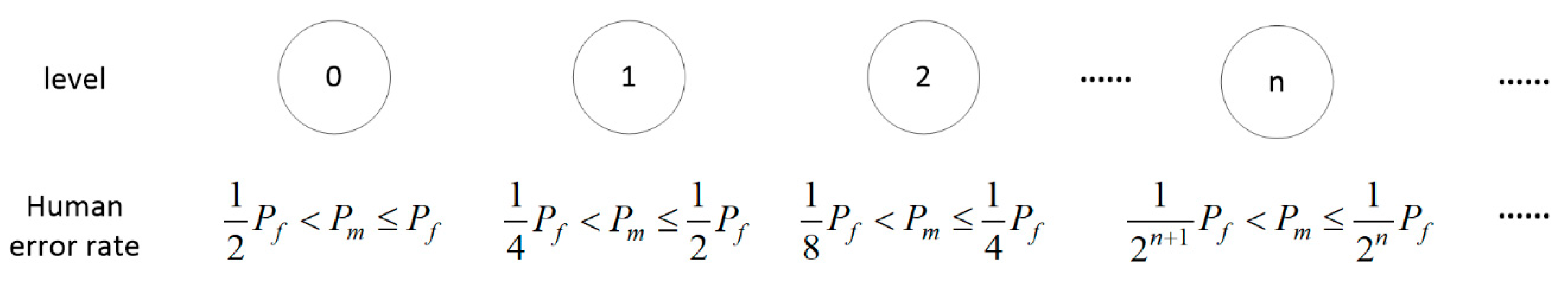
, so it is unnecessary to analyze different levels of human reliability. However, for MSSs and multi-state components, the failure of maintenance tasks does not mean that the system and its components have totally failed. Therefore, in order to establish the degradation model during the next mission, it is indispensable to determine the state distribution after maintenance if human error occurs. In this paper, we determine the human reliability level of maintenance workers by comparing P f and P m . Given the P f , whenever the P m (worker in lowest level when P m = P f ) drops by half, the level is considered to have changed. Figure 1 shows the human reliability level set.
In order to establish the selective maintenance optimization model, it is crucial to estimate the system reliability to perform the next mission. Let Z i denotes the state of component i after human error has occurred (the true state). First, determine the distribution of Z i according to the human reliability level of the maintenance worker. Second, analyze the degradation process of each component during the next mission. Then, with the constraints of maintenance resources, an optimization model can be established to obtain the optimal maintenance plan and select the suitable worker.

3.1. State Determination after Human Error

If the maintenance worker did not make a human error, the state of component i after the maintenance break is Y i ( Z i = Y i ). However, once a worker has made an error, Z i satisfies 0 Z i < Y i . Then, we use the conclusion of the BCG Experience Curve to estimate Z i . BCG Experience Curve refers to that there is a consistent correlation between the costs and total cumulative output. In short, if a production mission is executed repeatedly, its production cost will decrease. Each time the production is doubled, the cost (including management, marketing, distribution and manufacturing, etc.) will fall at a constant and measurable rate (approximately 10% to 30% per year). The proficiency of the workers is one of the most fundamental factors affecting the curve change. Yelle [29] made a detailed summary of the development history of the Experience Curve. According to the basic principle of the curve, an increase in production leads to an increase in the operational proficiency of workers, which in turn reduces production costs. High worker proficiency means lower HEP, which reduces operational losses due to human error. In this paper, human errors affect the state of components after maintenance, and thus affect the estimation of system reliability. Therefore, whether in a profit-oriented enterprise or a reliability-oriented industrial environment, a general conclusion is that the reduction of HEP will reduce unnecessary operational losses. Based on this theory, we apply the BCG Experience Curve in the distribution determination process after maintenance. The following assumptions are considered in this paper.
  • If human error occurs in a multi-state component i , the true state after maintenance Z i is lower than the target state ( 0 Z i < Y i ). The probability distribution of Z i is related to the human reliability level of the worker who performs the task during this maintenance break;
  • Experienced maintenance workers not only have lower HEP, but also have lower operational losses after human error occurs, i.e., the component has a higher probability of being in a better state when a human error occurs;
  • When P m satisfies P m = P f , the state of component i after human error satisfies Z i =   0 ;
  • Let P b denotes the transition rate between adjacent human reliability levels. The probability distribution of Z i is determined by P b and P m .
Let P m n ( Z i = B i ) denote the probability of Z i = B i ,   0 B i < Y i when the human reliability level is n . Clearly, B i = 0 Y i 1 P m n ( Z i = B i ) = 1 . If the human reliability level changes, the probability distribution of Z i will change accordingly, and P m n + 1 ( Z i =   B i ) in the new distribution is calculated by P m n ( Z i =   B i 1 ) P b + P m n ( Z i =   B i ) ( 1 P b ) , i.e., the probability of each state is transferred according to P b 
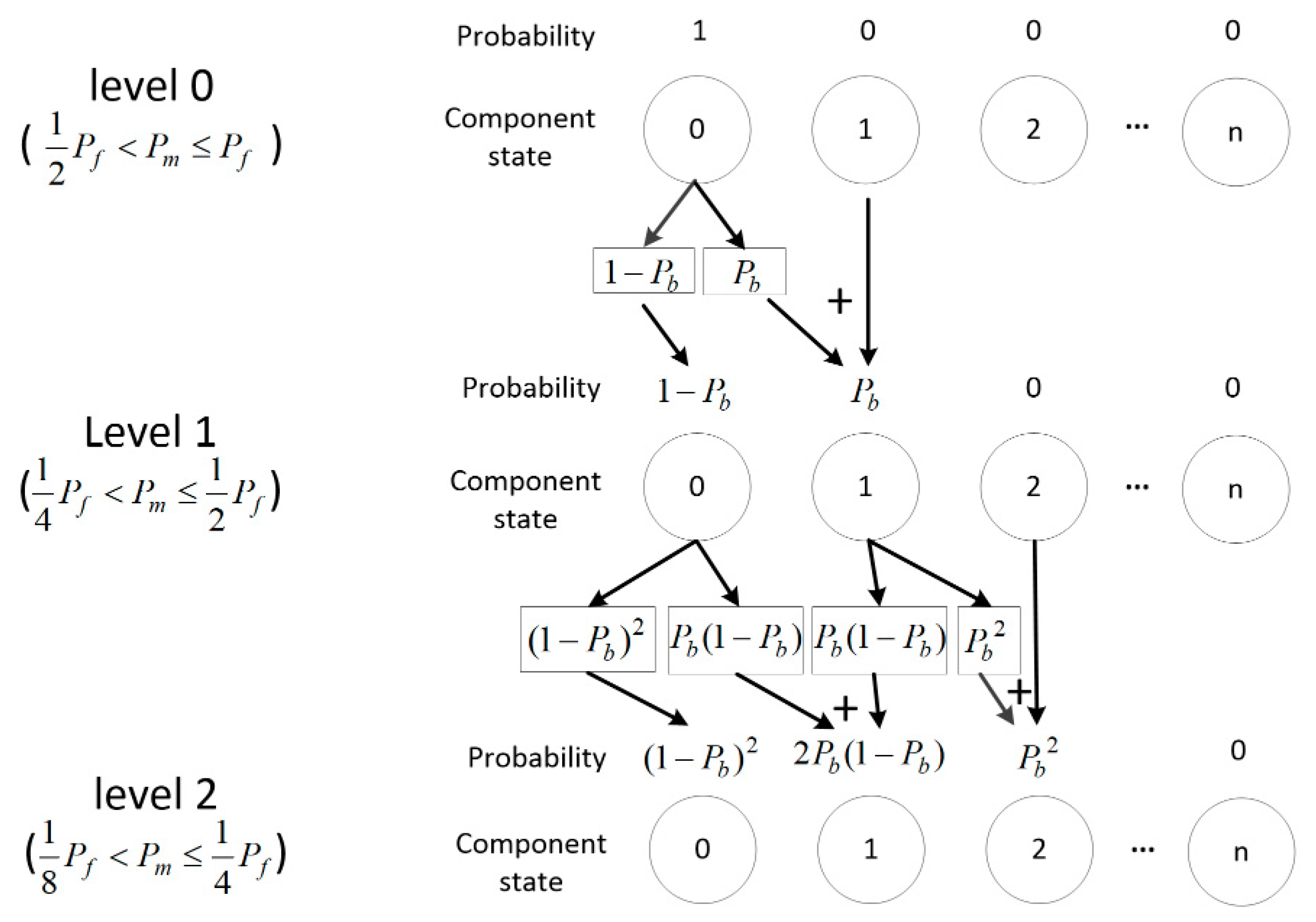
. Given the human reliability level set and P b , Figure 2 shows an example of the distribution determination process when the human reliability level changes from 0 to 2. The distribution of Z i in each level is given by Equations (14) to (17).
1 2 P f < P m P f { P m 0 ( Z i = 0 ) = 1 P m 0 ( Z i = 1 ) = P m 0 ( Z i = 2 ) = = P m 0 ( Z i , Y i 1 ) = 0
1 4 P f < P m 1 2 P f { P m 1 ( Z i = 0 ) = 1 P b P m 1 ( Z i = 1 ) = P b P m 1 ( Z i = 2 ) = P m 1 ( Z i = 3 ) = = P m 1 ( Z i = Y i 1 ) = 0    
1 8 P f < P m 1 4 P f { P m 2 ( Z i = 0 ) = ( 1 P b ) 2 P m 2 ( Z i = 1 ) = 2 P b ( 1 P b ) P m 2 ( Z i = 2 ) = P b 2 P m 2 ( Z i = 3 ) = P m 2 ( Z i = 4 ) = = P m 2 ( Z i = Y i 1 ) = 0
1 2 n 1 P f < P m 1 2 n P f   { P m n ( Z i = 0 ) = ( 1 P b ) n      P m n ( Z i = B i ) = P m n 1 ( Z i = B i 1 ) P b + P m n 1 ( Z i = B i ) ( 1 P b )      P m n ( Z i = n + 1 ) = P m n ( Z i = n + 2 ) = = P m n ( Z i = Y i 1 ) = 0
If n > Y i 1 , repeat Equation (17). According to the above equations (14) to (17), we can obtain the probability distribution of the state after a human error is made by maintenance worker m . Additionally, we can see that if P m is infinitely close to 0, we obtain Z i = Y i 1 . This conclusion is similar to that of the BCG Experience Curve. It means that the worker is more skilled and the HEP is lower, so the operational losses due to human error are also lower.
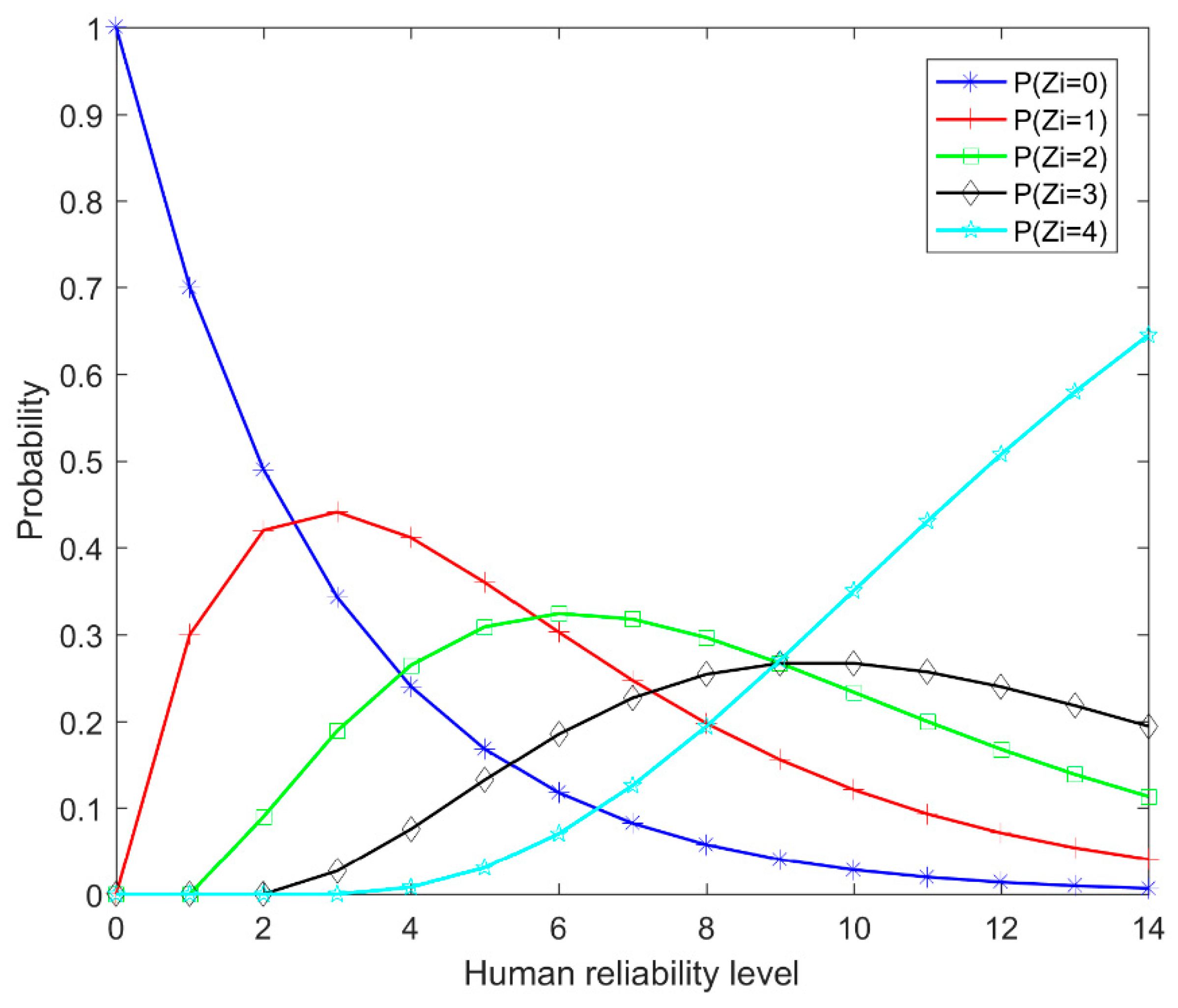
The following example is given to illustrate the working principle of this model. Consider a component that has six states, { 0 , 1 , 2 , 3 , 4 , 5 } , and the initial HEP is P f = 0.8 , the transition rate is P b = 0.3 , the initial state is 0, and the target state is 5. The probability that this component has different human reliability is shown in Figure 3. It can be seen that as the HEP decreases, there is a higher probability that the component will be in a higher state. If we use the selective maintenance model proposed in [24], the probability of components in different states after maintenance is equal for all workers, i.e., P m n ( Z i = B i ) = 0.2 , which is unable to reflect the different levels of workers. Table 1 shows the probability ranking of component i in each level.

3.2. Estimation of Component State Degradation and Multi-State System Reliability

The multi-state component degrades during the next mission. The degradation process of a multi-state component can be found in [14,30]. Assume that the components will not age during the maintenance break, and the degradation processes of all the components in the next mission are independent. As the mission progresses, the state of each component will progressively degrade, and the performance rate will also decrease. Let T denote the time required to perform the next mission. In this paper, the probability that component i with state r after maintenance by worker m degrading to state q at the end of the next mission, P r , q i ( T , m ) , is given. Since r = 0 , 1 , , K i and q = 0 , 1 , , r , the probabilities P r , q i ( T , m ) form a transition probability matrix in the next mission, which is given by:
[ 0 0 0 0 P 1 , 0 i P 1 , 1 i 0 0 P K i , 0 i P K i , 1 i P K i , K i 1 i P K i , K i i ] , i = 1 , 2 , , N
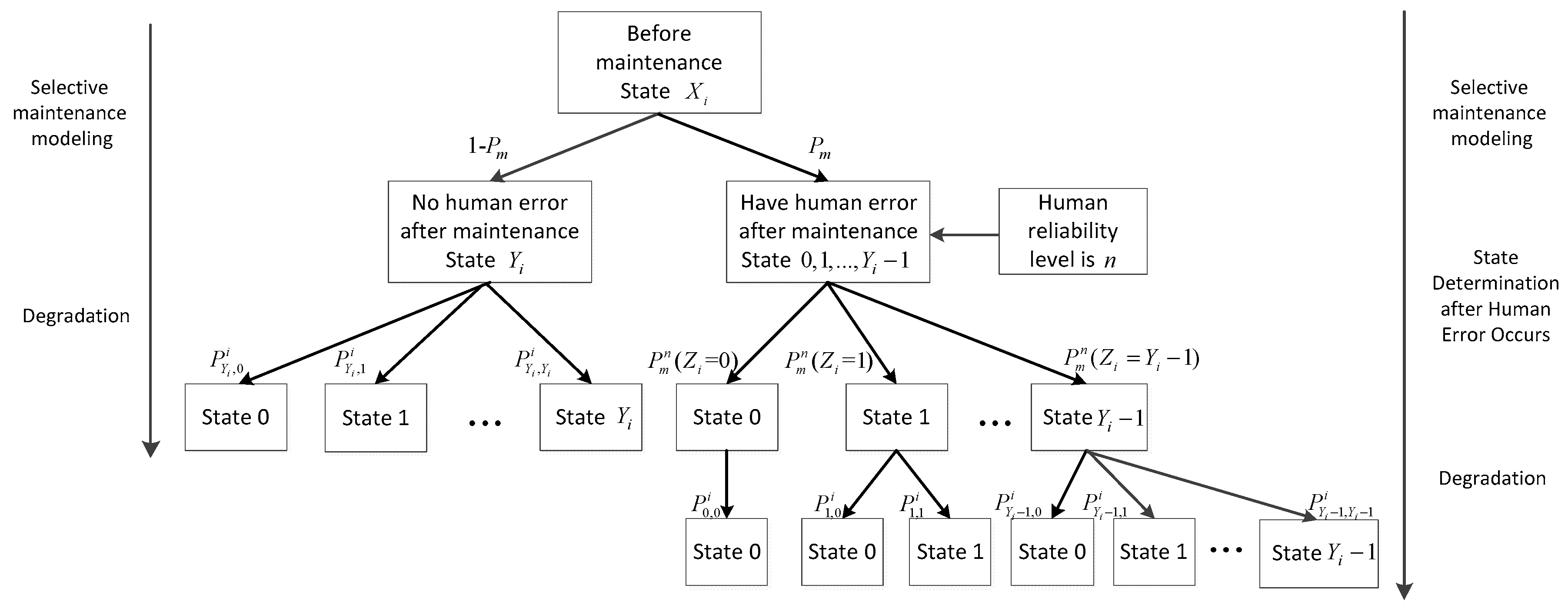
The state change process of component i between entering the maintenance break and the end of the next mission considering human reliability is shown in Figure 4. The probability of the next event occurring is marked next to the connecting lines.
The state distribution of components after the next mission is given by the universal generating function (UGF) (see [12,14,31]). The UGF is defined by Liu et al. [12] as a polynomial function to represent the probability mass function of a discrete random variable. For component i , the performance rate distribution at time t can be represented as:
u i , Y i ( v , t ) = j = 0 K i P Y i , j i ( t , m ) v g i , j i
According to equations (1) to (3) discussed in Section 2, the UGF of the overall system can be expressed by:
U Y ( v , t ) = Φ { j 1 = 0 K 1 [ ( 1 P m ) P Y 1 , j 1 1 ( t , m ) + P m Z 1 = 0 Y 1 1 P Z 1 , j 1 1 ( t , m ) ] v g 1 , j 1 ,   j 2 = 0 K 2 [ ( 1 P m ) P Y 2 , j 2 2 ( t , m ) + P m Z 2 = 0 Y 2 1 P Z 2 , j 2 2 ( t , m ) ] v g 2 , j 2 ,     ,   j N = 0 K N [ ( 1 P m ) P Y N , j N N ( t , m ) + P m Z N = 0 Y N 1 P Z N , j N N ( t , m ) ]   v g N , j N }
Equation (20) extends the UGF in [14] by considering human reliability. Clearly, if P m = 0 , the state after maintenance is Y i and the UGF is similar to that proposed in [14]. However, if P m > 0 , the state after maintenance follow a discrete distribution, which is proposed in Section 3.1. Therefore, the reliability of the system will decrease, since the performance is reduced.
As the performance rate decreases, the functioning level of the MSS gets worse. Whether the mission can be successfully completed depends on the performance rate of the MSS at the end of the next mission. Let W denote the performance rate requirement of the MSS at the end of the next mission. If G ( T ) is not less than W , the mission is considered successful. Therefore, the reliability of the MSS to perform the next mission is given by:
R M S S ( Y , T , W , m ) = G ( T ) W P J ( Y , T , m )
where Y = { Y 1 , Y 2 , , Y N } is the states vector set of all the components after maintenance, and J = { j 1 , j 2 , , j N } is the states vector set of all the components after degradation. Therefore, P J ( Y , T , m ) represents the probability that the state of the overall system is J at the end of the next mission. If the performance rate of state J is greater than W , the mission is considered successful, and vice versa.
Through Equation (21), we can obtain the system reliability under a selective maintenance plan Y considering human reliability.
For example, consider a simple MSS that consists of two components in parallel. Each component has three states, the performance rates of which are 0, 10, and 20, and the HEP of the maintenance worker is 0.1. According to equations (14) to (17), the probability that a component is in each state after human error occurs is P ( Z 1 =   0 ) = P ( Z 2 = 0 ) = 0.49 , P ( Z 1 =   1 ) =   P ( Z 2 = 1 ) = 0.51 . The state of each component entering the maintenance break is X = { 0 , 0 } and the target state is Y = { 2 , 2 } . The probabilities of degradation are P 0 , 0 1 =   1 , P 1 , 0 1 =   0.3 , P 1 , 1 1 =   0.7 , P 2 , 0 1 =   0.1 , P 2 , 1 1 =   0.3 , P 2 , 2 1 =   0.6 , P 0 , 0 2 =   1 , P 1 , 0 2 =   0.2 , P 1 , 1 2 =   0.8 , P 2 , 0 2 =   0.2 , P 2 , 1 2 =   0.3 , and P 2 , 2 1 =   0.5 . Therefore, the performance rate distribution of each component at time t can be represented as:
u 1 , 2 ( v , T ) = P 2 , 0 1 ( T , m ) v 0 + P 2 , 1 1 ( T , m ) v 10 + P 2 , 2 1 ( T , m ) v 20 = 0.1 v 0 + 0.3 v 10 + 0.6 v 20
u 2 , 2 ( v , T ) = P 2 , 0 2 ( T , m ) v 0 + P 2 , 1 2 ( T , m ) v 10 + P 2 , 2 2 ( T , m ) v 20 = 0.2 v 0 + 0.3 v 10 + 0.5 v 20
Therefore, the composition function is given by:
U Y ( v , t ) = min { [ 0.9 P 2 , 0 1 ( t , m ) + 0.1 × ( 0.49 P 0 , 0 1 + 0.51 P 1 , 0 1 ) ] v 0 + [ 0.9 P 2 , 1 1 ( t , m ) + 0.1 × 0.51 P 1 , 1 1 ) ] v 10 + 0.9 P 2 , 2 1 ( t , m ) v 20    , [ 0.9 P 2 , 0 2 ( t , m ) + 0.1 × ( 0.49 P 0 , 0 2 + 0.51 P 1 , 0 2 ) ] v 0 + [ 0.9 P 2 , 1 2 ( t , m ) + 0.1 × 0.51 P 1 , 1 2 ) ] v 10 + 0.9 P 2 , 2 2 ( t , m ) v 20 } = min { 0.1543 v 0 + 0.3057 v 10 + 0.54 v 20 , 0.2392 v 0 + 0.3108 v 10 + 0.45 v 20 } =   0.3566 v 0 + 0.4004 v 10 + 0.243 v 20
If the performance rate requirement of the MSS at the end of the next mission is 10, the reliability of the MSS to perform the next mission is 0.6434.

3.3. Optimization Model

Selective maintenance is a risky policy, since some components of the system cannot be perfectly functional in the next mission. Additionally, the risk of the selective maintenance is further increased by human error. In such a case, a suitable maintenance worker must be selected for this maintenance task. The optimization model in this paper is for finding the best selective maintenance subset for maximizing the probability of successfully completing the next mission. The associated integer decision variable is Y i . Let T L and C L denote the maintenance time and costs limitation. The resulting nonlinear optimization problem is given by:
P :   Maximiz      R M S S ( Y , T , W , m ) = G ( T ) W P J ( Y , T , m )
i = 1 N T i T L
Subject   to          i = 1 N C i C L
X i Y i K i
Y i   is   integer ,   i = 1 , 2 , , N
In the above formulations, the objective of function (25) is to maximize the reliability of the overall system under the maintenance by worker m , which has been formulated in Section 3.2. Constraints (26) and (27) exhibit the limited available maintenance resources to perform maintenance. The calculation method of T i and C i is given in Section 2.2. Constraints (28) and (29) show that the state after maintenance must be an integer value between X i and the maximum state K i for all i = 1 , 2 , , N , since the maintenance does not worsen the state of the components. For a given MSS’s configuration, this nonlinear optimization problem can be solved. The following section presents an example and discusses how the human reliability may have an important impact on the selective maintenance model. In this experiment, the duration and costs are given in time and monetary units, respectively.
Different maintenance workers have different HEPs, and not all workers are qualified for the maintenance task. After the model gives the optimal maintenance plan, let R ^ M S S denotes the reliability of the system without considering human reliability, and let R L be the minimum acceptable reliability for the MSS to perform the next mission considering human reliability. Then, R L can be calculated by:
R L =   α R ^ M S S
where α   ( 0 < α < 1 ) represents the risk factor for human error, with a higher value of α indicating a higher requirement for human reliability.
For a maintenance worker m , if the optimal reliability satisfies R M S S ( Y , T , W , m ) R L given by the optimization model, the worker can be selected to perform maintenance tasks. Since this is a typical constrained nonlinear optimization problem involving integer variables only, a genetic algorithm (GA) is employed to solve the discrete mathematics problem in this paper. More details about GA can be found in [32].

4. Case Analysis

Consider a multi-state series-parallel system (Figure 5) consisting of 10 components that are numbered 1 to 10. Components 1, 4, and 10 have five states, while Components 2, 3, 5, 6, 7, 8, and 9 have four states. The overall system consists of six subsystems, which are numbered 1 to 6. Subsystems 1, 3, and 6 consist of only one component; Subsystems 2 and 4 consist of two components, and Subsystem 5 consists of three components. The basic information of the maintenance task in this break is shown in Table 2. The maintenance time and costs for each component are shown in Table 3. The degradation information of all the components after the next mission is shown in Table 4. The information of three maintenance workers ( M =   3 ) is shown in Table 5. The parameters of the genetic algorithms are shown in Table 6. For this maintenance break, the state set before maintenance is X = { 0 , 1 , 1 , 1 , 0 , 1 , 2 , 1 , 0 , 1 } .
According the calculation method given in 
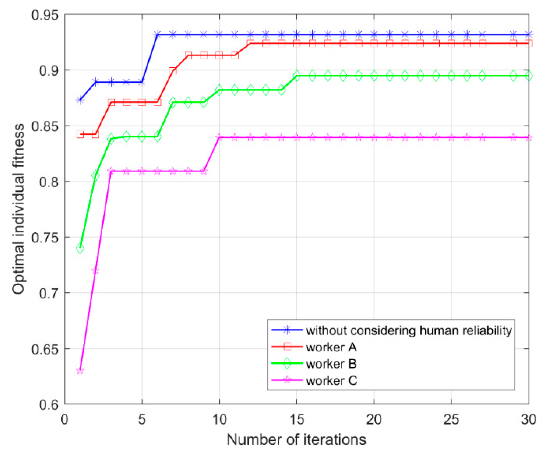
Section 2.3, the HEPs of three maintenance workers in this paper are 0.0166, 0.0544, and 0.1174, respectively, and the genetic algorithm program was run multiple times using the MATLAB software (MathWorks, Natick, MA, USA). The results are shown in Table 7 and Figure 6. The optimal maintenance plan is found to be Y = { 4 , 2 , 1 , 4 , 3 , 3 , 2 , 3 , 1 , 4 } , and the optimal maintenance options were found to be “Repair” for Components 1, 4, 5, 6, 8, and 10, “Imperfect Maintenance” for Components 2, 7, and 9, and “Do Nothing” for Component 3. The time and costs required for the optimal selective maintenance plan are 533 units and 182 units, respectively. The reliability of the optimal selective maintenance plan for the system to perform the next mission without considering human reliability is 0.9316. According to Table 7, the reliability of the MSS after maintenance by workers A, B, and C is 0.9239, 0.8948, and 0.8391, respectively. Clearly, the system reliability will be reduced when human reliability is taken into account in the selective maintenance optimization model, i.e., ignoring human error will lead to overestimation of the system performance rate at the end of the next mission. According to the maintenance information given in Table 2, the minimum reliability requirement for the MSS considering human reliability is 0.9037. If the system reliability after considering human reliability is greater than 0.9037, the maintenance worker can perform the maintenance task; otherwise, the worker needs to be replaced with a more qualified worker. Clearly, worker A meets the minimum reliability requirements, and can perform this maintenance task. However, workers B and C do not meet the minimum reliability requirements. If maintenance worker B or C is responsible for the maintenance task without considering the human reliability, the optimal reliability will be 0.9316 after solving the optimization model. This value is seriously overestimated compared to the true reliability, and does not meet the minimum reliability requirements ( R L ). If the maintenance task is still carried out by maintenance worker B or C, the performance rate of the MSS at the end of the next mission may not meet the requirements, resulting in unnecessary operational losses.
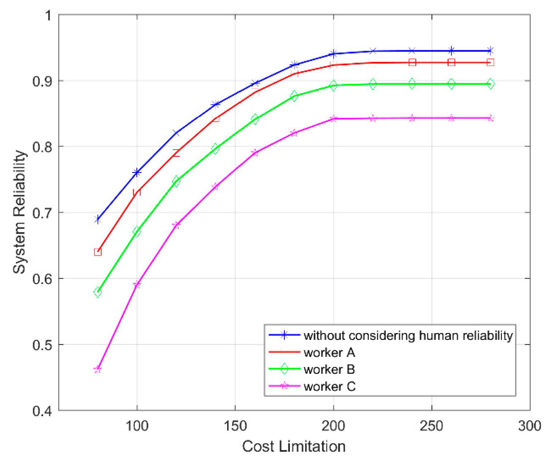
In this case, the maintenance resources and performance rate requirement ( W ) are factors that affect the reliability of the MSS to perform the next mission, and also affect the selection of the maintenance worker. Loose resource limitations reduce the risk of selective maintenance and reduce the requirements of HEP for maintenance workers. However, tighter resource limitations lead to a lower system reliability.
In this case, the maintenance time and costs of all the components are 688 and 221, respectively. Figure 7 and Figure 8 show the effect of human reliability under different constraints of maintenance time and costs. When comparing different time limitations, it is considered that there is no limit on the costs. Similarly, time limitations are not considered when comparing different cost limitations. As the limitations become tighter, the reliability of the system becomes lower, and the higher the HEP is, the faster the reliability decreases. This indicates that the error is magnified when the limitation of resources is tighter.
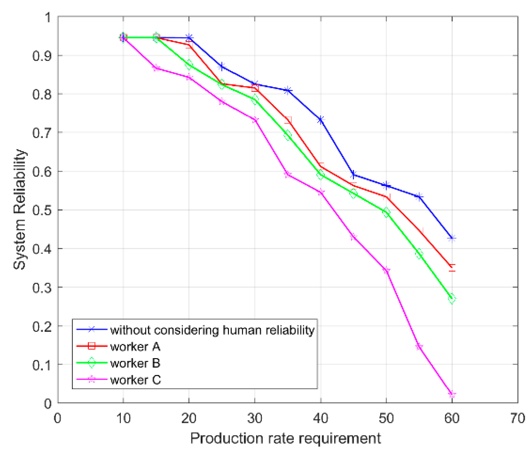
Figure 9 shows the system reliability under different performance rate requirements. It can be seen that the tighter the requirements, the lower the reliability of the system, the higher the HEP of the maintenance workers, and the faster the reliability decreases.
By comparing the system reliability with different limitations of time, costs, and performance rate, the importance of considering human reliability is fully proven. When the limitations are tighter, the impact of human reliability on the system reliability is more obvious.

5. Conclusions

A selective maintenance model for an MSS considering human reliability was investigated for the first time in this paper. We formulated the relationships between the HEP and the state of components after maintenance using a dynamic discrete distribution and a model proposed to calculate the HEP. A method to determine the distribution of component states after maintenance was also proposed. A reliability evaluation for the MSS was performed by using a UGF for different maintenance options that depends on the available maintenance resources and human reliability level. A generalized selective maintenance optimization model was developed to maximize the system reliability in the next mission considering both time and cost constraints. The maintenance model helps maintenance decision makers decide the best combination of maintenance activities and suitable workers to maximize the system reliability in the next mission within the available time and budget. An illustrative example is presented, and the discrete mathematics optimization problem is solved using a genetic algorithm, and selective maintenance strategies considering and not considering human reliability are analyzed. The results demonstrate that ignoring human reliability may lead to the overestimation of system reliability, and this error is magnified when the limitation of resources and the performance rate requirement are tighter. The proposed selective maintenance model can be applied to many industrial and military situations where it is crucial to allocate limited resources during a maintenance break. Further extension of the model to consider multiple maintenance workers for one maintenance break is a suitable topic for future research. Another interesting future research topic could be the development of multiple missions in a planning horizon using a selective maintenance model that takes human reliability into account. Finally, considering uncertain data in human reliability modeling (such as [33,34]) can also help to estimate the system reliability accurately, which is important for further research.

Author Contributions

Conceptualization, Z.Z. and N.W.; Methodology, Z.Z. and N.W.; Formal analysis, N.W. and B.X.; Software, X.Y. and N.W.; Validation, B.X. and L.M.; Writing–Original Draft Preparation, Z.Z.; Supervision, L.M.

Funding

This research received no external funding.

Conflicts of Interest

The authors declare no conflict of interest.

Notation

N total number of components in an MSS
i index of components, i = 1 , 2 , , N
L number of subsystems in an MSS
l index of subsystems, l = 1 , 2 , , L
N l number of components in subsystem l
S i the state set of the component i , S i = ( 0 , 1 , , K i 1 , K i )
Φ composition operator for all components
X states vector set of all components before maintenance, X = { X 1 , X 2 , , X N }
Y states vector set of all components after maintenance, Y = { Y 1 , Y 2 , , Y N }
J states vector set of all components at the end of the next mission, J = { j 1 , j 2 , , j N }
Z i state of component i after human error occurs, X i Z i < Y i
T i maintenance time of component i during maintenance break
C i maintenance costs of component i during maintenance break
T L maintenance time limit
C L maintenance costs limit
g i , j performance rate of component i in state j , j = 0 , 1 , 2 , K i
g i ( t ) performance rate of component i at time t
G l ( t ) performance rate of subsystem l at time t
G ( t ) performance rate of an MSS at time t
M number of maintenance workers available
m index of maintenance workers, m = 1 , 2 , , M
P m human error probability of maintenance worker m
P Y i , j i ( t , m ) the probability of component i degrading from state Y i to state j i at time t after maintenance by worker m , j i = 0 , 1 , , Y i
u i , Y i ( v , t ) universal generating function for component i in state Y i at time t
U Y ( v , t ) universal generating function for an MSS in state Y at time t
T time required to perform next mission
W the requirement of performance rate at the end of next mission
R M S S reliability of MSS to perform the next mission considering human reliability
R ^ M S S reliability of MSS to perform the next mission without considering human reliability
R L minimum reliability required for next mission
M E number of years of maintenance experience
M Q total number of human errors
M T influence of maintenance environment on maintenance time
M C the state difference before and after maintenance ( Y i X i )

References

  1. Rice, W.F.; Cassady, C.R.; Nachlas, J.A. Optimal maintenance plans under limited maintenance time. In Proceedings of the Seventh Industrial Engineering Research Conference, Banff, AB, Canada, 9–10 May 1998. [Google Scholar]
  2. Cassady, C.R.; Murdock, W.P., Jr.; Pohl, E.A. Selective maintenance for support equipment involving multiple maintenance actions. Eur. J. Oper. Res. 2001, 129, 252–258. [Google Scholar] [CrossRef]
  3. Cassady, C.R.; Pohl, E.A.; Murdock, W.P. Selective maintenance modeling for industrial systems. J. Qual. Maint. Eng. 2001, 7, 104–117. [Google Scholar] [CrossRef]
  4. Maillart, L.M.; Cassady, C.R.; Rainwater, C.; Schneider, K. Selective maintenance decision-making over extended planning horizons. IEEE Trans. Reliab. 2009, 58, 462–469. [Google Scholar] [CrossRef]
  5. Schneider, K.; Cassady, C.R. Evaluation and comparison of alternative fleet-level selective maintenance models. Reliab. Eng. Syst. Saf. 2015, 134, 178–187. [Google Scholar] [CrossRef]
  6. Yang, D.; Wang, M.S.H.; Feng, Q.; Ren, Y.; Sun, B.; Wang, Z. Fleet-level selective maintenance problem under a phased mission scheme with short breaks: A heuristic sequential game approach. Comput. Ind. Eng. 2018, 119, 404–415. [Google Scholar] [CrossRef]
  7. Diallo, C.; Venkatadri, U.; Khatab, A.; Liu, Z. Optimal selective maintenance decisions for large serial, k -out-of- n:G, systems under imperfect maintenance. Reliab. Eng. Syst. Saf. 2018, 175, 234–245. [Google Scholar] [CrossRef]
  8. Duan, C.; Deng, C.; Gharaei, A.; Wu, J.; Wang, B. Selective maintenance scheduling under stochastic maintenance quality with multiple maintenance actions. Int. J. Prod. Res. 2018, 56, 1–19. [Google Scholar] [CrossRef]
  9. Khatab, A.; Aghezzaf, E.H.; Diallo, C.; Djelloul, I. Selective maintenance optimisation for series-parallel systems alternating missions and scheduled breaks with stochastic durations. Int. J. Prod. Res. 2017, 55, 3008–3024. [Google Scholar] [CrossRef]
  10. Ali, I.; Raghav, Y.S.; Khan, M.F.; Bari, A. Selective maintenance in system reliability with random costs of repairing and replacing the components. Commun. Stat. Simul. Comput. 2013, 42, 14. [Google Scholar] [CrossRef]
  11. Chen, J.; Meng, Q.H.; Zuo, M.J. Selective maintenance optimization for multi-state systems. In Proceedings of the 1999 IEEE Canadian Conference on Electrical and Computer Engineering, Edmonton, AB, Canada, 9–12 May 1999; pp. 1477–1482. [Google Scholar]
  12. Liu, Y.; Huang, H.Z. Optimal selective maintenance strategy for multi-state systems under imperfect maintenance. IEEE Trans. Reliab. 2010, 59, 356–367. [Google Scholar] [CrossRef]
  13. Lisnianski, A.; Levitin, G. Multi-State System Reliability, Assessment, Optimization and Applications; World Scientific Publishing Company: Singapore, 2003. [Google Scholar]
  14. Pandey, M.; Zuo, M.J.; Moghaddass, R. Selective maintenance modeling for a multi-state system with multi-state components under imperfect maintenance. Iie Trans. 2013, 45, 1221–1234. [Google Scholar] [CrossRef]
  15. Nakagawa, T. Optimum policies when preventive maintenance is imperfect. IEEE Trans. Reliab. 1979, 28, 331–332. [Google Scholar] [CrossRef]
  16. Nakagawa, T. Imperfect preventive-maintenance. IEEE Trans. Reliab. 1979, 28, 402. [Google Scholar] [CrossRef]
  17. Pham, H. Imperfect maintenance. Eur. J. Oper. Res. 1996, 94, 425–438. [Google Scholar] [CrossRef]
  18. Dao, C.D.; Zuo, M.J.; Pandey, M. Selective maintenance for multi-state series–parallel systems under economic dependence. Reliab. Eng. Syst. Saf. 2014, 121, 240–249. [Google Scholar] [CrossRef]
  19. Dao, C.D.; Zuo, M.J. Selective maintenance of multi-state systems with structural dependence. Reliab. Eng. Syst. Saf. 2017, 159, 184–195. [Google Scholar] [CrossRef]
  20. Lust, T.; Roux, O.; Riane, F. Exact and heuristic methods for the selective maintenance problem. Eur. J. Oper. Res. 2009, 197, 1166–1177. [Google Scholar] [CrossRef]
  21. Xu, Q.; Guo, L.; Wang, N. Selective maintenance model and its solution algorithm for multi-state series-parallel system under economic dependence. In Proceedings of the Control & Decision Conference, Yinchuan, China, 28–30 May 2016. [Google Scholar]
  22. Moieni, P.; Spurgin, A.J.; Singh, A. Advances in human reliability analysis methodology. Part I: Frameworks, models and data. Reliab. Eng. Syst. Saf. 1994, 44, 27–55. [Google Scholar] [CrossRef]
  23. Zaitseva, E.; Puuronen, S. Multi-state system in human reliability analysis. In Proceedings of the Conference on Human System Interactions, Catania, Italy, 21–23 May 2009; pp. 657–660. [Google Scholar]
  24. Zhao, Z.; Yan, X.; Xiao, B.; Sun, X. Selective maintenance modeling for a multi-state system considering human reliability. In Proceedings of the 3rd International Conference on System Reliability and Safety (ICSRS), Barcelona, Spain, 24–26 November 2018; pp. 346–352. [Google Scholar]
  25. Hollnagel, E. Cognitive Reliability and Error Analysis Method; Elsevier Science Ltd.: Oxford, UK, 1998. [Google Scholar]
  26. Kontogiannis, T. A framework for the analysis of cognitive reliability in complex systems: A recovery centred approach. Reliab. Eng. Syst. Saf. 1997, 58, 233–248. [Google Scholar] [CrossRef]
  27. Nourelfath, M.; Fitouhi, M.; Machani, M. An integrated model for production and preventive maintenance planning in multi-state systems. IEEE Trans. Reliab. 2010, 59, 496–506. [Google Scholar] [CrossRef]
  28. Kim, J.W.; Jung, W. A taxonomy of performance influencing factors for human reliability analysis of emergency tasks. J. Loss. Prevent. Proc. 2003, 16, 479–495. [Google Scholar] [CrossRef]
  29. Yelle, L.E. The learning curve: Historical review and comprehensive survey. Decis. Sci. 2010, 10, 302–328. [Google Scholar] [CrossRef]
  30. Dao, C.D.; Zuo, M.J. Selective maintenance for multi-state series systems with s-dependent components. IEEE Trans. Reliab. 2016, 65, 525–539. [Google Scholar] [CrossRef]
  31. Levitin, G. The Universal Generating Function in Reliability Analysis and Optimization; Springer: London, UK, 2005. [Google Scholar]
  32. Sivanandam, S.N.; Deepa, S.N. Introduction to Genetic Algorithms; Springer: Berlin/Heidelberg, Germany, 2008. [Google Scholar]
  33. Mkrtchyan, L.; Podofillini, L.; Dang, V.N. Methods for building conditional probability tables of bayesian belief networks from limited judgment: An evaluation for human reliability application. Reliab. Eng. Syst. Saf. 2016, 151, 93–112. [Google Scholar] [CrossRef]
  34. Zaitseva, E.; Levashenko, V.; Kvassay, M.; Barach, P. Healthcare system reliability analysis addressing uncertain and ambiguous data. In Proceedings of the International Conferende on Information and Digital Technologies, Zilina, Slovakia, 5–7 June 2017; pp. 442–451. [Google Scholar]
Figure 1. Human reliability level set of maintenance workers.
Symmetry 11 00652 g001
Figure 2. An example of the distribution determination process.
Symmetry 11 00652 g002
Figure 3. Probability of a component in different human reliability levels.
Symmetry 11 00652 g003
Figure 4. State change process of components.
Symmetry 11 00652 g004
Figure 5. Structure of the system.
Symmetry 11 00652 g005
Figure 6. Operation result of genetic algorithm.
Symmetry 11 00652 g006
Figure 7. Multi-state system (MSS) reliability under different time constraints.
Symmetry 11 00652 g007
Figure 8. MSS reliability under different cost constraints.
Symmetry 11 00652 g008
Figure 9. MSS reliability under different performance rate requirements.
Symmetry 11 00652 g009
Table 1. The probability ranking of different human reliability levels.
LevelHuman Error ProbabilityProbability Ranking
0 0.4 < P m 0.8 P ( Z i = 0 ) > P ( Z i = 1 ) = P ( Z i = 2 ) = P ( Z i = 3 ) = P ( Z i = 4 )
1 0.2 < P m 0.4 P ( Z i = 0 ) > P ( Z i = 1 ) > P ( Z i = 2 ) = P ( Z i = 3 ) = P ( Z i = 4 )
2 0.1 < P m 0.2 P ( Z i = 0 ) > P ( Z i = 1 ) > P ( Z i = 2 ) > P ( Z i = 3 ) = P ( Z i = 4 )
3 0.05 < P m 0.1 P ( Z i = 1 ) > P ( Z i = 0 ) > P ( Z i = 2 ) > P ( Z i = 3 ) > P ( Z i = 4 )
4 0.025 < P m 0.5 P ( Z i = 1 ) > P ( Z i = 2 ) > P ( Z i = 0 ) > P ( Z i = 3 ) > P ( Z i = 4 )
5 0.0125 < P m 0.025 P ( Z i = 1 ) > P ( Z i = 2 ) > P ( Z i = 0 ) > P ( Z i = 3 ) > P ( Z i = 4 )
6 0.00625 < P m 0.0125 P ( Z i = 2 ) > P ( Z i = 1 ) > P ( Z i = 3 ) > P ( Z i = 0 ) > P ( Z i = 4 )
7 3.125 × 10 3 < P m 0.00625 P ( Z i = 2 ) > P ( Z i = 1 ) > P ( Z i = 3 ) > P ( Z i = 4 ) > P ( Z i = 0 )
8 1.56 × 10 3 < P m 3.125 × 10 3 P ( Z i = 2 ) > P ( Z i = 3 ) > P ( Z i = 1 ) > P ( Z i = 4 ) > P ( Z i = 0 )
9 7.8 × 10 4 < P m 1.56 × 10 3 P ( Z i = 4 ) > P ( Z i = 3 ) = P ( Z i = 2 ) > P ( Z i = 1 ) > P ( Z i = 0 )
10–14 P m 7.8 × 10 4 P ( Z i = 4 ) > P ( Z i = 3 ) > P ( Z i = 2 ) > P ( Z i = 1 ) > P ( Z i = 0 )
Table 2. Maintenance information.
T L   ( Units ) C L   ( Units ) M λ 1 λ 2 P f P b W α
54018530.500.500.500.30200.97
Table 3. Component information.
Component IDComponent Information
StatePerformance RateMaintenance Time/Costs (Units)
01234
1000/038/764/1391/27121/40
120-0/026/653/2083/33
240--0/027/1457/27
365---0/030/13
495----0/0
2000/032/956/2076/31-
130-0/024/1144/22-
250--0/020/11-
370 0/0-
3000/025/848/1683/20-
125-0/023/858/4-
245--0/035/4-
370---0/0-
4000/033/1268/25108/40140/51
140-0/035/1375/28107/39
275--0/040/1572/26
390---0/032/11
4125----0/0
5000/019/636/1055/15-
120-0/017/436/9-
235--0/019/5-
350---0/0-
6000/022/844/1767/26-
125-0/022/945/18-
235--0/023/9-
355---0/0-
7000/015/331/745/11-
115-0/016/430/8-
225--0/014/4-
340---0/0-
8000/023/744/1563/23-
130-0/021/840/16-
250--0/019/8-
375---0/0-
9000/031/1060/1994/30-
125-0/029/963/20-
240--0/034/11-
355 --0/0-
10000/032/1265/2399/33140/45
135-0/033/1169/21110/33
260--0/036/1077/22
395---0/041/12
4115----0/0
Table 4. Component degradation information.
Com IDInitial State State after MaintenanceDegradation Probability
01234
10010000
10.200.80000
20.150.240.6100
30.050.150.280.520
40.020.090.140.260.49
2101000-
10.300.7000-
20.120.220.660-
30.050.110.270.57
3101000-
10.130.8700-
20.080.320.600-
30.060.240.340.36
41010000
10.170.83000
20.090.160.7500
30.050.110.210.630
40.010.040.110.240.60
5001000-
10.420.4800-
20.270.350.380-
30.160.220.290.33-
6101000-
10.300.7000-
20.160.240.600-
30.080.120.350.55-
7201000-
10.350.6500-
20.220.310.470-
30.140.200.290.37-
8101000-
10.440.5600-
20.180.380.440-
30.030.090.300.58-
9001000-
10.140.8600-
20.120.250.630-
30.080.140.270.51-
101010000
10.270.73000
20.150.230.6200
30.060.120.200.620
40.010.030.130.180.65
Table 5. Maintenance worker information.
Worker IDParameter
M E M Q V M T E d P m
A2511200.9540.0166
B155600.9030.0544
C55350.8030.1174
Table 6. Genetic algorithm parameters.
Population SizeNumber of IterationsMutation ProbabilityCrossover ProbabilityGeneration Gap
100300.010.70.9
Table 7. Optimal maintenance plan.
Component IDTarget StateOptionTime (Units)Costs (Units) R ^ M S S R L Reliability Considering Human Reliability
ABC
14Repair5331820.93160.90370.92390.89480.8391
22Imperfect Maintenance
31Do Nothing
44Repair
53Repair
63Repair
72Imperfect Maintenance
83Repair
91Imperfect Maintenance
104Repair

