Buffer Occupancy-Based Transport to Reduce Flow Completion Time of Short Flows in Data Center Networks

Abstract

Today’s data centers host a variety of different applications that impose specific requirements for their flows. Applications that generate short flows are usually latency sensitive; they require their flows to be completed as fast as possible. Short flows suffer to quickly increase their sending rate due to the existing long flows occupying most of the available capacity. This problem is caused due to the slow convergence of the current data center transport protocols. In this paper, we present a buffer occupancy-based transport protocol (BOTCP) to reduce flow completion time of short flows. BOTCP consists of two parts: (i) A novel buffer occupancy-based congestion signal, and (ii) a congestion control scheme that uses the congestion signal to reduce flow completion time of short flows. The proposed buffer occupancy-based congestion signal gives a precise measure of congestion. The congestion control scheme makes a differentiated treatment of short and long flows to reduce flow completion time of short flows. The results show that BOTCP significantly improves flow completion time of short flows over the existing transport protocols in data center networks.

1. Introduction

Internet services and applications are growing at a rapid pace. These services and applications are hosted on large-scale computation and storage infrastructure called data center (DC). A data center contains a large number of computation and storage servers interconnected by a specifically designed network, named data center network (DCN). A data center network not only serves as communication infrastructure but can also play a critical role in optimizing data center operations [1]. It hosts a range of applications from present day Internet apps, like Web search, audio/video streaming, social networking, etc., to compute intensive applications, like meteorology programs, to communication intensive applications like MapReduce [2,3,4,5,6,7].

Data centers are growing at a rapid pace and the DCN server count is increasing exponentially. In Microsoft, the rapid growth in the number of users and the amount of data to be processed and stored cause the number of servers, in the datacenter, to double every 14 months [6]. In addition, since hundreds of servers in a datacenter network work together to generate user response, like response to a user query, generating a user page etc., the intra-DCN traffic is increasing at a faster rate than the Internet traffic. To generate HTML code of a requested Web page in Facebook’s datacenter, an average of 130 internal requests are made [5]. Datacenters consume a significant amount of energy produced by the entire world. In 2013, 91 billion kilowatt-hours of energy was consumed by United States (US) datacenters, which accounts to 1.5% of the total energy consumed by the country [8].

The services and applications hosted in large-scale data centers impose an ever-increasing demand for throughput and/or latency requirements. These services and applications may lose profits of millions of dollars due to even a small lapse in the performance. A delay of 100 ms causes a 1% reduction in Amazon’s sales. An additional delay of 0.5 s in generating response to a Google search query caused 20% reduction in their traffic [9]. Therefore, efficient performance, in terms of latency, is a critical requirement for these services [3,4,10]. In addition, some unique characteristics differentiate datacenter networks from the Internet, like: (i) Single administrative domain, (ii) multiple paths between a pair of end-hosts, (iii) bursty traffic, (iv) many-to-one communication pattern, and (v) small buffer sizes at switches. Therefore, solutions that are deployed in the Internet cannot always be effective and efficient in datacenter networks, as well [11].

Some studies [12,13,14] have analyzed traffic characteristics of DCNs and argued that datacenter flows can be broadly categorized into short and long flows. Flow size of more than 80% flows is less than 10 KB, but around 90% of the total DCN traffic belongs to long flows. Web search query and Web page retrieving tasks generate a number of short flows. Data update, data backup, and VM migration tasks produce long flows. Short flows are latency/flow completion time (FCT) sensitive, and long flows are throughput sensitive. Short flows arrive in large numbers [15] and remain alive for a very small period of time, whereas long flows are very few but remain alive for a much longer period of time [12,13,14]. Since long flows remain in the network for a much longer period of time, they acquire all the available capacity of the path in the absence of short flows; in this case, when short flows arrive they suffer to quickly increase their sending rates due to the slow convergence of the existing data center transport protocols [4], this causes significant increase in flow completion times of short flows which ultimately results in inefficient response time for the application. Figure 1 shows a simplified scenario of bandwidth usage by short and long flows. At first, there were only two long flows consuming all the available capacity. Later, five short flows arrived to compete for the same path. As most of the available capacity is held by the long flows, the short flows suffer to quickly increase their sending rates. This results in inefficient flow completion times of short flows, which ultimately turns into in poor performance of the related applications.

In this paper, a buffer occupancy-based transport protocol (BOTCP) is proposed. BOTCP consists of two key components: (i) A new buffer occupancy-based congestion signal and (ii) a congestion control scheme based on the proposed congestion signal. BOTCP is implemented by making certain changes in the existing TCP’s congestion signal and congestion control scheme. It aims to: Minimize packet drops, achieve high utilization, and reduce flow completion time of short flows without compromising overall throughput of long flows. The results show that BOTCP effectively reduces flow completion time of short flows over the most widely used datacenter transport protocols.

The rest of the paper is structured as follows. The next section discusses related work. The design rationale of BOTCP is presented in Section 3. Section 4 gives the details of BOTCP. Implementation and a comparison of results with the two most commonly used datacenter network transport protocols (i.e., TCP and DCTCP) are presented in Section 5. The paper is concluded in Section 6.

2. Related Work

Many solutions have been proposed by researchers to improve latency/flow completion time of flows. These solutions can be categorized on the basis of the technique they employed.

The authors of [16,17] tried to reduce flow completion time by improving the congestion signal. The authors of [16] proposed to combine explicit congestion notification (ECN) and round-trip time (RTT) to form a new congestion signal, specifically, ECN as a per-hop signal and RTT as an end-to-end queuing delay signal. Datacenter networks, however, have RTTs on the scale of up to few hundred microseconds, and, as pointed out in [18,19], most operating systems lack fine-grained microsecond-level timers. Hence an RTT-based congestion signal is not very feasible in most current DCNs. The authors of [17] proposed a new congestion signal named Combined Enqueue and Dequeue Marking (CEDM). CEDM modified ECN marking by introducing: (i) Marking decision at two time points (i.e., packet enqueue and packet dequeue time), and (ii) two threshold values (K₁ and K₂). The scheme focused only on the buffer underflow problem and did not address the packet drop issue due to buffer overflow, which adversely affects flow completion times.

The authors of [20,21] proposed window-based explicit bandwidth allocation schemes. The authors of [20] named their scheme SAB (sharing by allocating switch buffer); the scheme works as such: Switch tracks the current number of flows that compete for the same output port and allocates congestion windows to flows such that the sum of the traffic from all the flows remains greater than the bandwidth delay product (BDP) and less than the buffer capacity at the output port of the switch. This simultaneously ensures high utilization and minimum packet losses. Due to the maintenance of the number of active flows, the switches ensure fairness by allocating capacity to flows as buffer size divided by number of flows. In addition, switches can reduce flow completion time/latency by taking a smaller value for buffer size. The authors of [21] aimed to achieve the objectives of zero queueing, rare packet drops, and fast convergence. The scheme proposed to determine flow pipeline capacity without buffer space, this allows a switch to allocate capacities to flows in such a way to achieve the three objectives. Both of these schemes require the network fabric to track and maintain state information of flows in order to explicitly assign flow rates. The schemes may suffer from scalability issues in large-scale data centers due to limited memory resources at switches [22].

The authors of [4,23] leveraged from the fact that, in datacenter networks, multiple paths exist between each pair of edge switches. The authors of [4] replicated a TCP-SYN (handshake) over multiple paths and used the one that completed first. They also replicated short flows and used whichever finished first. The scheme does not require any changes in switching fabric and protocol stack but builds on top of Equal-Cost Multi-Path routing (ECMP) for selecting a different path for the second connection. Studies [24,25] show that ECMP induces congestion when hash collisions occur and performs inefficiently in asymmetric topologies. The authors of [23] proposed a multilayer solution to improve the latency of flows. They broadcasted a TCP-SYN packet to find and select the fastest path to the destination. The scheme required state information to be stored at switches. The scheme selected the best (fastest) path to destination, and since data centers exhibit bursty flow arrivals due to many-to-one communication pattern, the best path could be easily congested in the event of Incast traffic [26].

Study [27] proposed a scheme to reduce flow completion times of short flows using ECN marking as a congestion signal. The authors tried to approximate Least Attained Service (LAS) scheduling by adjusting (i.e., increasing or decreasing) the congestion window based on the parameter ‘data sent so far’; that is, the congestion window of short flows is increased relatively more than long flows, and in the event of congestion, long flows back off more than short flows. The scheme employs ECN marking for the congestion signal. ECN marking only tells whether the queue length is greater than a certain threshold level or not; it does not inform about the exact magnitude/degree of congestion; therefore, ECN-based schemes suffer from frequent packet drops and, consequently, inefficient performance.

Study [28] proposed certain changes in TCP and named their solution ‘Data Center TCP’ (DCTCP). DCTCP makes changes in the ECN mechanism by marking packets based on instantaneous queue length. When marked bits are received at sender (in acknowledgements), the congestion window is reduced to the extent of the number of marked packets received rather than being reduced to half as is done in ECN-enabled TCP. DCTCP claims to have better burst tolerance, flow completion time, and throughput than TCP. The results of the proposed scheme will be compared with TCP and DCTCP—the two most widely deployed transport protocols in today’s data centers.

3. Design Rationale

There are two necessary components for a scheme to reduce flow completion time of short flows: (i) An accurate and effective congestion signal and (ii) an efficient scheme that uses the congestion signal to effectively reduce flow completion time of short flows. Here, we first propose a new congestion signal then discuss a transport scheme to reduce flow completion time of short flows using the proposed congestion signal.

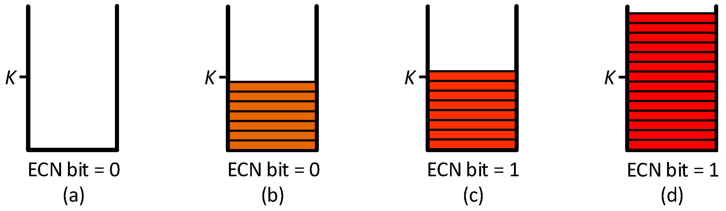
3.1. Proposed Congestion Signal

As discussed in the previous section, DCN round-trip times (RTTs) are on the scale of up to a few hundred microseconds and most operating systems lack fine-grained microsecond level timers. In addition, an RTT-based congestion signal is not very effective if there exist multiple bottlenecks along the path of the flow [16,17]. Hence, an RTT-based congestion signal is not suitable in most current DCNs. Similarly, ECN marking is the core congestion signal used in most of the current data center transport solutions (e.g., DCTCP). The ECN scheme checks the queue length against a certain threshold (K) and marks the ECN bit in the packet if the queue length is equal or above the threshold. As shown in Figure 2, the ECN bit is zero if the buffer occupancy is zero up to just less than the threshold; similarly, the bit is marked if the buffer occupancy is just above the threshold up to the maximum buffer capacity at the output port of the switch. Thus, the scheme does not give a precise measure of buffer occupancy, i.e., the extent of congestion. This causes frequent packet drops in the ECN-based transport schemes and consequently results in performance degradation.

Having exact information of buffer occupancy at the output port of the bottleneck link can give a precise measure of congestion along the path, which can enable us far better control over preventing packet drops. In such a scheme, a flow’s rate can be increased or decreased, proportionate to the value of the buffer occupancy at the bottleneck link. In large-scale datacenter networks, servers are interconnected through commodity switches. These switches have 64–256 KB buffers associated with each output port [28]. In addition, a typical 1500 bytes maximum transmission unit (MTU) is used in datacenter networks. The lower-order 10 bits of queue length do not offer any information about the number of packets in the queue and, hence, can be ignored. Thus, the bits higher than the lower-order 10 bits give us the measure of buffer occupancy on the scale of packets. This value of buffer occupancy can be propagated to the source end-host by introducing an option in the IP header’s options field.

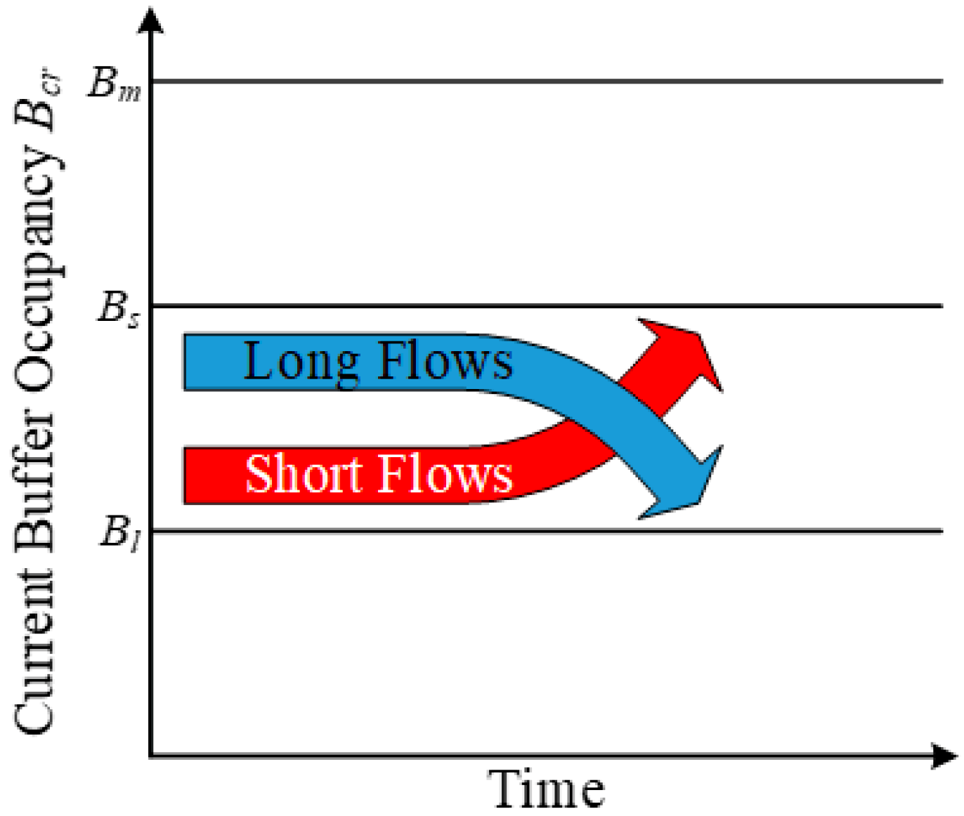
3.2. Design of Buffer Occupancy-Based Transport

The objective is to design a transport scheme that: (i) Minimizes packet drops while keeping high utilization, and (ii) reduces flow completion time of short flows without compromising overall throughput of long flows. The idea here is to: (i) Control the flows’ rate so as to keep the buffer occupancy, at switch, at a certain level, and (ii) treat short and long flows differently.

Inflight data consists of data (packets) in queues and data travelling along links. There can be many bottleneck links along the path of a flow but one of them will have the highest value of buffer occupancy, we call it bottleneck link.

Let

• C_b = buffer capacity at output port of bottleneck link
• B_cr = current buffer occupancy at output port of bottleneck link
• B_s = allowed buffer occupancy at output port of bottleneck link, for short flows
• B_l = allowed buffer occupancy at output port of bottleneck link, for long flows
• B_m = maximum allowed buffer occupancy at output port of bottleneck link
• N = number of flows with same bottleneck link
• BDP_i = bandwidth-delay product of path of flow i
• D_i = current value of amount of data that the flow i is allowed to send in one RTT, i.e., congestion window of flow i represented in units of MSS

such that,

B_l < B_s < B_m < C_b

Different flow loads are defined as follows:

• Normal flow load: If D_i ≥ 1 MSS ∀ i ∊ {1, 2, …, N} and B_cr ≤ B_s.
• Heavy flow load: If D_i ≥ 1 MSS ∀ i ∊ {1, 2, …, N} and B_s < B_cr ≤ B_m.
• Extreme flow load: If D_i < 1 MSS ∀ i ∊ {1, 2, …, N} and B_cr > B_s.

In normal flow load, the sending rate (D_i) of flow i is adjusted to bring B_cr to either B_s (if flow i is short) or B_l (if flow i is long). In the case of heavy load, the sending rate of both types of flows is kept at 1 MSS till B_cr is in the range B_s < B_cr ≤ B_m. In extreme flow load, the sending rate of both types of flows is adjusted to bring B_cr to B_m such that D_i remains ≤ 1 MSS.

In the following two subsections, we discuss sending rates of long and short flows. The initial sending rate of both types of flows is 1 MSS. An increase or decrease in the sending rate of a flow depends on its type, value of B_cr, and current sending rate (D_i). For ease of reference, we divide the possible scenarios into cases.

3.2.1. Sending Rate of Long Flows

Case l1: If B_cr ≤ B_l and D_i ≥ 1 MSS then sending rate is increased to bring B_cr to B_l.

Case l2: If B_l < B_cr ≤ B_s and D_i > 1 MSS then sending rate is decreased to bring B_cr to B_l unless the resultant value becomes less than 1 MSS, in which case the sending rate (D_i) is assigned a value of 1 MSS. If B_l < B_cr ≤ B_s and D_i = 1 MSS then the sending rate is not changed and is kept at 1 MSS.

Case l3: If B_s < B_cr ≤ B_m and D_i > 1 MSS then the sending rate is halved unless the resultant value becomes less than 1 MSS, in which case the sending rate (D_i) is assigned a value of 1 MSS. If B_s < B_cr ≤ B_m and D_i = 1 MSS then the sending rate is not changed and is kept at 1 MSS.

Case l4: If B_cr > B_m and D_i ≥ 1 MSS then the sending rate is halved.

Case l5: If B_cr > B_m and D_i < 1 MSS then the sending rate is decreased to bring B_cr to B_m.

Case l6: If B_cr ≤ B_s and D_i < 1 MSS then the sending rate is doubled unless the resultant value becomes greater than 1 MSS, in which case the sending rate (D_i) is assigned a value of 1 MSS.

Case l7: If B_s < B_cr ≤ B_m and D_i < 1 MSS then the sending rate is increased to bring B_cr to B_m unless the resultant value becomes greater than 1 MSS, in which case the sending rate (D_i) is assigned a value of 1 MSS.

3.2.2. Sending Rate of Short Flows

Case s1: If B_cr ≤ B_s and D_i ≥ 1 MSS then the sending rate is increased to bring B_cr to B_s.

Case s2: If B_s < B_cr ≤ B_m and D_i > 1 MSS then the sending rate is decreased to bring B_cr to B_s unless the resultant value becomes less than 1 MSS, in which case the sending rate (D_i) is assigned a value of 1 MSS. If B_s < B_cr ≤ B_m and D_i = 1 MSS then the sending rate is not changed and is kept at 1 MSS.

Cases s3, s4, s5, and s6 for short flows are same as cases l4, l5, l6, and l7 for long flows, respectively.

The following two lemmas show how to adjust the sending rate to bring B_cr to B_l as discussed in cases l1 and l2 for long flows.

Lemma 1.

If B_cr < B_l, then the long flows with the same bottleneck link may increase (B_l − B_cr) the amount of data, or each flow may increase its sending rate by$D_i\times \frac{B_l-B_{cr}}{B_{cr}}$amount of data.

Proof. 

Buffer occupancy with D_i amount of data sent = B_cr.

Buffer occupancy with $D_i\left(1+\frac{B_l-B_{cr}}{B_{cr}}\right)$ amount of data sent = $\frac{B_{cr}}{D_i}\times D_i\left(1+\frac{B_l-B_{cr}}{B_{cr}}\right)=B_l$.  □

Lemma 2.

If B_l < B_cr ≤ B_s then the long flows with the same bottleneck link may decrease (B_cr − B_l) the amount of data, or each flow may decrease its sending rate by$D_i\times \frac{B_{cr}-B_l}{B_{cr}}$amount of data.

Proof. 

Buffer occupancy with D_i amount of data sent = B_cr.

Buffer occupancy with $D_i\left(1-\frac{B_{cr}-B_l}{B_{cr}}\right)$ amount of data sent = $\frac{B_{cr}}{D_i}\times D_i\left(1-\frac{B_{cr}-B_l}{B_{cr}}\right)=B_l$.  □

In case l1, as shown in lemma 1, D_i is assigned the value $D_i\left(1+\frac{B_l-B_{cr}}{B_{cr}}\right)$. In case l2, as shown in lemma 2 and as per the condition in case l2, D_i is assigned the value $MAX\left(D_i\left(1-\frac{B_{cr}-B_l}{B_{cr}}\right),1\right)$. Cases l7, s1, and s6 are dealt with similar to lemma 1. Cases l5, s2, and s4 are dealt with similar to lemma 2.

In the discussion of flow loads, cases l1, l2, and s1 fall in normal load. Cases l3 and s2 come in heavy load. Cases l4, l5, l6, l7, s3, s4, s5, and s6 fall in extreme flow load. In a normal flow load, short and long flows are treated differently. In heavy and extreme flow loads, short and long flows are treated the same. Flow completion time of short flows is reduced in normal load. The aim in heavy and extreme flow loads is to allow flows to continue sending data without causing packet drops.

3.3. Reducing Flow Completion Time of Short Flows

As discussed, flow completion time of short flows is reduced in a normal flow load. Here, the key scenario occurs when only long flows are running and short flows arrive to compete for the same bottleneck link. Here, case l2 occurs for long flows and case s1 occurs for short flows. As shown in Figure 3, long flows reduce their sending rates to bring B_cr to B_l and short flows increase their sending rate to bring B_cr to B_s; that is, each long flow decreases by $D_i\times \frac{B_{cr}-B_l}{B_{cr}}$ amount of data and each short flow increases by $D_i\times \frac{B_s-B_{cr}}{B_{cr}}$ amount of data in each RTT until the sending rate of long flows is reduced to 1 MSS. Thus, in each RTT, the bandwidth share shifts from long flows to short flows. The sending rate of long flows is not reduced below 1 MSS to prevent long flows from starvation.

3.4. Minimizing Packet Drops and Achieving High Utilization

The objective of minimizing packet drops is achieved by keeping buffer occupancy at bottleneck link (B_cr) around B_m even in the event of extreme flow load. High utilization is achieved by choosing B_l such that: B_l ≥ 2 × MAX (BDP₁, BDP₂, …, BDP_N).

3.5. Overall Throughput of Long Flows

The throughput of long flows is decreased only for the duration of short flows. As soon as the short flows finish, long flows reclaim all the available bandwidth. As studies [12,13,14] suggest, the short flows remain alive only for a small period of time. Therefore, the overall throughput of long flows does not experience significant degradation.

4. Buffer Occupancy-Based Transport

In this section, a buffer occupancy-based transport protocol (BOTCP) to reduce flow completion time of short flows in data center networks is presented. BOTCP makes certain changes in TCP, specifically: (i) A new congestion signal, named buffer occupancy feedback (BOF), is used instead of ECN marking, and (ii) a new, BOF-based, congestion control (BOCC) scheme is employed. The objective of a buffer occupancy-based congestion signal (BOF) is to have precise information about congestion along the path so that it can be effectively used to minimize packet drops. The objectives of the buffer occupancy-based congestion control (BOCC) scheme is to: (i) Minimize packet drops while keeping high utilization, and (ii) reduce flow completion time of short flows without compromising overall throughput of long flows. The two parts of BOTCP are discussed in detail subsequently.

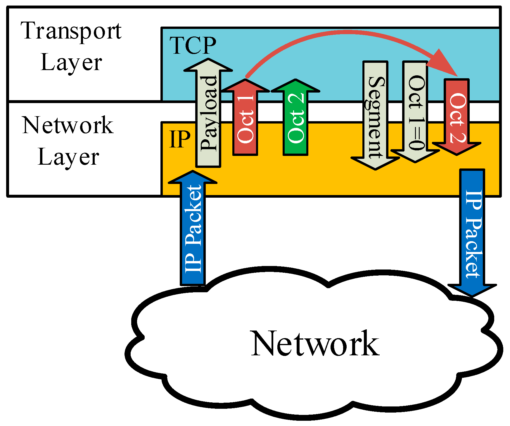
4.1. Buffer Occupancy Feedback (BOF)

We require the buffer occupancy at the output port of the bottleneck link. As discussed in the previous section, this information can be obtained from the higher-order bits of the queue length value at the output port of switch.

For buffer occupancy feedback, we add a 4-byte option to the IP header options and name it “buffer-occupancy-feedback” option. The options format has three fields: One octet for option-type (for option identification), one octet for option-length (in bytes), and the remaining octets for option-data (two bytes in our case). The option-type octet is further divided into three fields: (i) 1-bit copied flag, (ii) 2-bit option class, and (iii) 5-bit option number; we specify a unique option-type value that is not already used by another option to identify the buffer-occupancy-feedback option at the switches (e.g., copied flag = (1)₂ = 1, option class = (11)₂ = 3, option number = (00010)₂ = 2, thus, option-type = (11100010)₂ = 226). The option-length octet is assigned a value of (00000100)₂ = 4. In addition to the data segment, the transport protocol hands over to IP protocol two 1-byte values for the first and second octet of option-data, separately. The switches along the path update only the first octet of option-data (i.e., the third octet in the 4-byte buffer-occupancy-feedback option). At destination, the IP protocol hands over the values in the two octets of option-data to the transport layer in addition to the payload (i.e., the data segment). The value in the first octet of option-data is updated at switches along the forward path from the source and thus is required at the source; hence, the transport protocol at destination, hands-over this value as the second octet (i.e., the fourth octet in the buffer-occupancy-feedback option) to the IP protocol to be dispatched to the source. This value (buffer occupancy) is received at the source and is used in the congestion control scheme. In short, for each received packet on one end of the connection, the host uses the value in the second octet in its congestion control and echoes the value in the first octet to the other end of the connection as shown in Figure 4; the other end would use this value in its congestion control scheme.

We name the first octet of buffer-occupancy-feedback option-data as “BOF” field. The BOF field in the packet is updated at a switch, as shown in Figure 5. A switch along the path compares the BOF field, in the packet’s IP header, with the higher-order bits of buffer occupancy (BO) of the output port (i.e., the bits that describe the queue length on the scale of packets), and overwrites the value in the BOF field, in the packet, with the BO if BO is greater than the current value in the BOF field.

4.2. Buffer Occupancy-Based Congestion Control (BOCC)

Procedures 1 to 4 calculate sender’s congestion window. Procedure 1 is the main procedure that calls other procedures to increase or decrease the congestion window. Procedure INCREASE_CONGESTION_WINDOW (B) is called if cw ≥ 1 MSS and B_cr is less than or equal to B_l (for long flows) or B_s (for short flows). It is aligned with the cases l1 and s1 discussed in the previous section. This procedure increases the congestion window to bring B_cr to either B_l or B_s (depending to the flow type). Procedure DECREASE_CONGESTION_WINDOW (B₁, B₂) decreases the congestion window and is called if cw ≥ 1 MSS and B_cr is greater than B_l (for long flows) or B_s (for short flows). It is aligned with cases l2, l3, l4, s2, and s3. The key scenario occurs when cw ≥ 1 MSS and B_l < B_cr ≤ B_s; now with each received acknowledgement, long flows decrease their congestion windows as ‘MAX (cw − ((B_cr − B_l)/B_cr), 1)’ and short flows increase their congestion windows as ‘cw + ((B_s − B_cr)/B_cr)’. Thus, in each RTT, the bandwidth share shifts from long flows to short flows. Procedure SUB_MSS_CONGESTION_WINDOW () is called if cw < 1 MSS. It is aligned with cases l5, l6, l7, s4, s5, and s6. This procedure increases the congestion window if B_cr ≤ B_m and decreases the congestion window if B_cr > B_m; the increase is only allowed if the resultant congestion window is less than or equal to 1 MSS, otherwise congestion window is assigned a value of 1 MSS.

Procedure 1: CONGESTION_WINDOW_CALCULATION

Global Constants

Allowed buffer occupancy for short flows ‘Bs’

Allowed buffer occupancy for long flows ‘Bl’

Maximum allowed buffer occupancy ‘Bm’

Global Variables

Current buffer occupancy ‘Bcr’

Congestion window ‘cw’

Flow type ‘ft’     ▷ flow type is ‘short’ by default and is turn to ‘long’ after X number of bytes sent

Procedure CONGESTION_WINDOW ()

1 IF cw ≥ 1

2   IF ft = ‘short’

3     IF Bcr ≤ Bs

4       INCREASE_CONGESTION_WINDOW (Bs)

5     ELSE

6       DECREASE_CONGESTION_WINDOW (Bs, Bm)

7   ELSE

8     IF Bcr ≤ Bl

9       INCREASE_CONGESTION_WINDOW (Bl)

10     ELSE

11       DECREASE_CONGESTION_WINDOW (Bl, Bs)

12 ELSE

13   SUB_MSS_CONGESTION_WINDOW ()

Procedure 2: INCREASE_CONGESTION_WINDOW (B)

1   IF (Bcr × 2) ≤ B

2     cw ← cw + 1

3   ELSE

4     cw ← cw + ((B − Bcr)/Bcr)

Procedure 3: DECREASE_CONGESTION_WINDOW (B1, B2)

1 IF (Bcr > B1) AND (Bcr ≤ B2)

2   cw ← MAX (cw − ((Bcr − B1)/Bcr), 1)

3 ELSE

4   IF ft = ‘long’

5     IF (Bcr > Bs) AND (Bcr ≤ Bm)

6       cw ← MAX ((cw − 0.5), 1)

7     ELSE

8       cw ← cw − 0.5

9   ELSE

10     cw ← cw − 0.5

Procedure 4: SUB_MSS_CONGESTION_WINDOW ()

1 IF Bcr ≤ Bs

2   IF (Bcr × 2) ≤ Bs

3     cw ← cw × 2

4   ELSE

5     cw ← MIN (cw × 2, 1)

6 ELSE

7   IF (Bcr > Bs) AND (Bcr ≤ Bm)

8     cw ← MIN (cw × (1 + ((Bm − Bcr)/Bcr)), 1)

9   ELSE

10     cw ← cw × (1 − ((Bcr − Bm)/Bcr))

4.3. Short vs Long Flows

The size of short flows is defined roughly in the range 1–100 KB. The size of long flows is defined as ≥100 KB [12,13,14]. Therefore, we use a simple method to differentiate between short and long flows. A flow type variable ft is maintained for each flow. Each new flow is a short flow by default. When the number of bytes sent so far exceeds a threshold value X (e.g., 50 KB), then the flow type is updated to long flow.

4.4. Overhead

The BOTCP introduces a 4-byte buffer-occupancy-feedback option in the IP header of the packet. In a typical DCN, with a size of 1500 bytes for the data packet, the overhead introduced by BOTCP is 4/1456 = 0.2747%.

4.5. Time Complexity

Time complexity of BOTCP will be discussed in comparison with TCP and DCTCP and their congestion signal, i.e., ECN. BOTCP consists of buffer occupancy feedback (BOF) and BOF-based congestion control (BOCC). Time complexity of BOF is the same as that of the ECN mechanism, i.e., O(1), since no loops or recursive function calls are involved as shown in Figure 5.

The time complexity of BOCC depends on two things. First, the time complexity of the congestion window update function, and second, the number of calls to the update function. The time complexity of BOCC’s congestion window update function is the same as that of TCP and DCTCP, i.e., O(1), since again there are no loops or recursive function calls. The number of calls to the update function depends on the number of packets, i.e., the BOCC’s congestion window update function is called each time an acknowledgement is received. In comparison, in TCP and DCTCP, the congestion window update function is called once per congestion window. Therefore, in the worst case, the time complexity of BOCC increases relative to the time complexity of TCP and DCTCP by a constant factor of BDP of the path/packet size. Since data center networks have very small propagation delays, i.e., on the scale of a few microseconds (µs), BDP of the path/packet size results in a small value.

4.6. Same Treatment of Short and Long Flows

There are two possible scenarios when short and long flows get the same treatment.

• Heavy and extreme flow load: In both heavy and extreme flow loads, the short and long flows are treated indifferently.
• Short and long flows start at same time: Short and long flows are differentiated on the basis of the amount of sent data. Hence, each new flow is treated as a short flow in the beginning until the data sent exceeds a specified number of bytes. Therefore, if short and long flows start at around same time, then long flows will be treated as short flows.

5. Results and Discussion

BOTCP is implemented in the network simulator ns-2 and a comprehensive set of simulation experiments is carried out to evaluate the performance of BOTCP. The proposed scheme is also compared with TCP with ECN marking option and DCTCP [28], the two most widely deployed DCN transport protocols.

The simulation experiments are carried out using various topologies and workloads. As an example, a symmetric 6 × 6 leaf-spine topology is created with an oversubscription ratio of 3:2 at leaf level. 32 hosts are connected to each leaf switch by 10-Gbps links making a total of 192 hosts. Each leaf switch is connected to each spine switch with a 40-Gbps link. The buffer size at a switch’s output port is taken to be 128 KB. A typical packet size of 1500 bytes is used, which makes a maximum queue limit of ~87 packets. The threshold value to change flow type from short to long is set to 10 KB. B_l, B_s, and B_m are set to 20, 40, and 60, respectively. Similarly, the ‘threshold value’ for TCP (with ECN) and ‘K’ for DCTCP are set to 20. minRTO for all the three schemes is set to 0.2 ms.

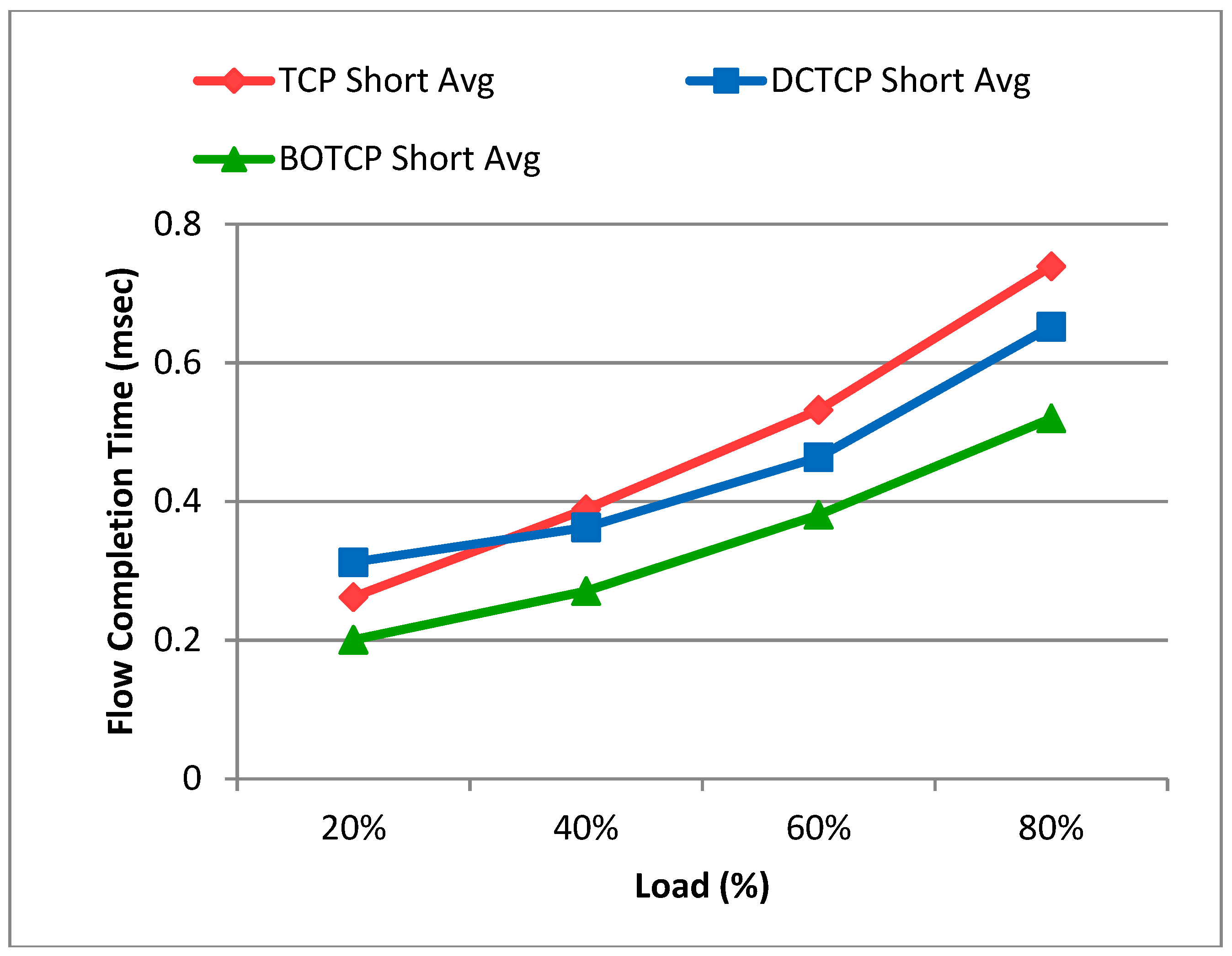
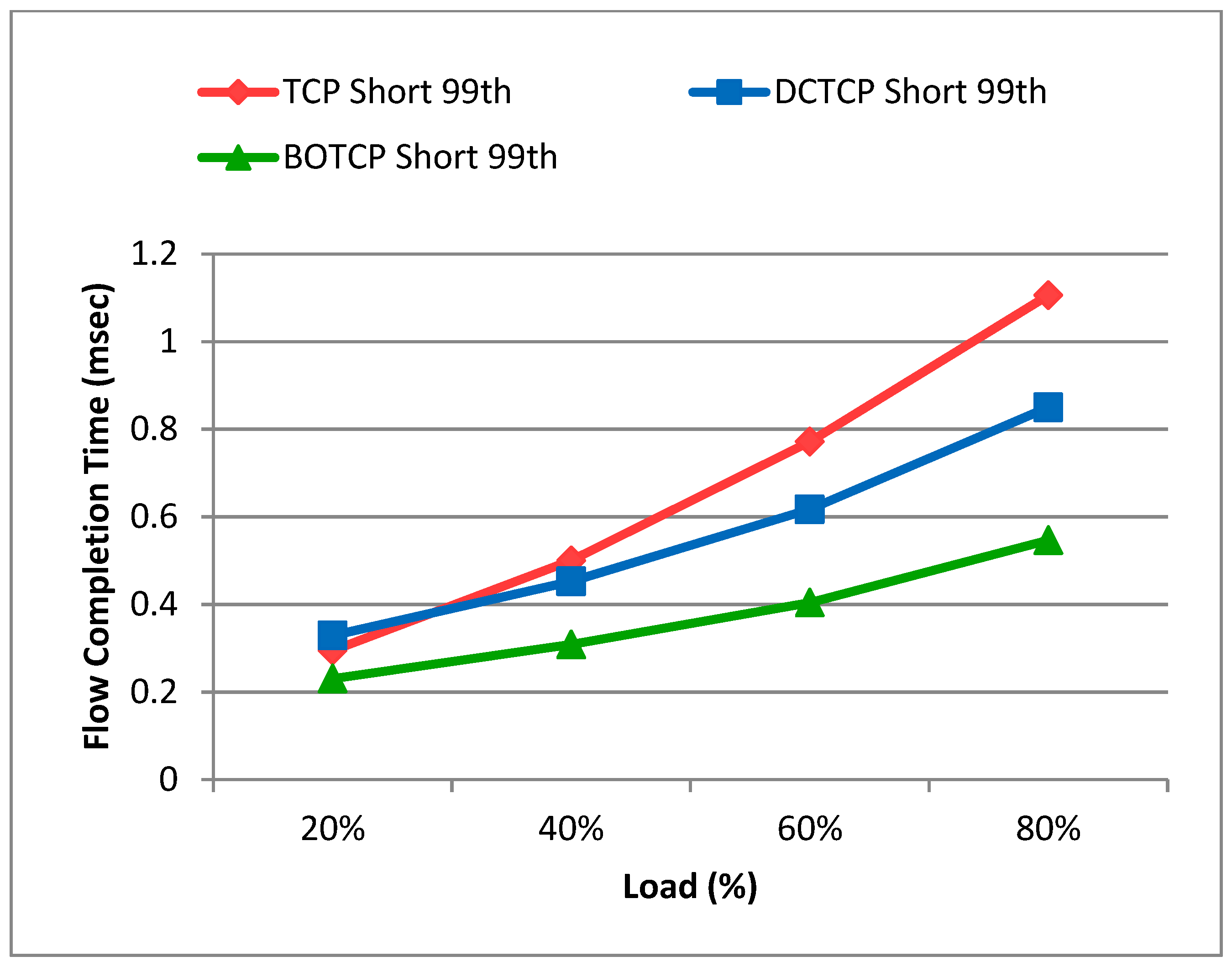
5.1. Flow Completion Time of Short Flows

BOTCP improves average and 99th percentile of FCT, of short flows, over both TCP and DCTCP, as shown in the graphs of Figure 6 and Figure 7. There are two factors to BOTCP’s better performance than TCP and DCTCP. First, priority treatment of short flows; second, minimizing the chances of packet drops. In BOTCP, short flows quickly acquire bandwidth from long flows; hence, short flows finish earlier than in TCP and DCTCP. In addition, BOTCP has exact information of buffer occupancy at the bottleneck link through its buffer occupancy-based congestion signal (BOF). BOTCP uses this information to opportunely adjust the sending rates and hence minimizes the chances of packet drops.

Under lighter loads, TCP (with the ECN congestion signal) performs better than DCTCP, as shown in the graphs of Figure 6 and Figure 7. This is due to two reasons: (i) DCTCP aims for low variance in the congestion window, and (ii) no packet drops occur under lighter loads. DCTCP reduces the congestion window proportional to the fraction of packets marked in the previous RTT. Thus, when new (short) flows join to share the same bottleneck link, there is a smaller reduction in the sending rates of existing (long) flows in each RTT, resulting in slower growth of sending rates of new flows than in TCP.

Under heavier loads DCTCP performs better than TCP. This is because DCTCP suffers from packets drops less than TCP does. DCTCP makes a subtle change in the ECN mechanism by marking the ECN bit in packets based on the instantaneous queue length instead of the average queue length. Therefore, in DCTCP, packets are marked on the basis of a relatively more accurate value of queue length than in the original ECN.

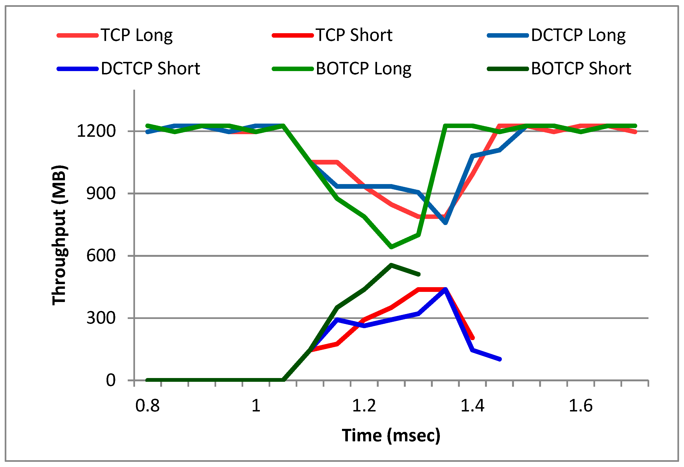
5.2. Bandwidth Sharing between Short and Long Flows

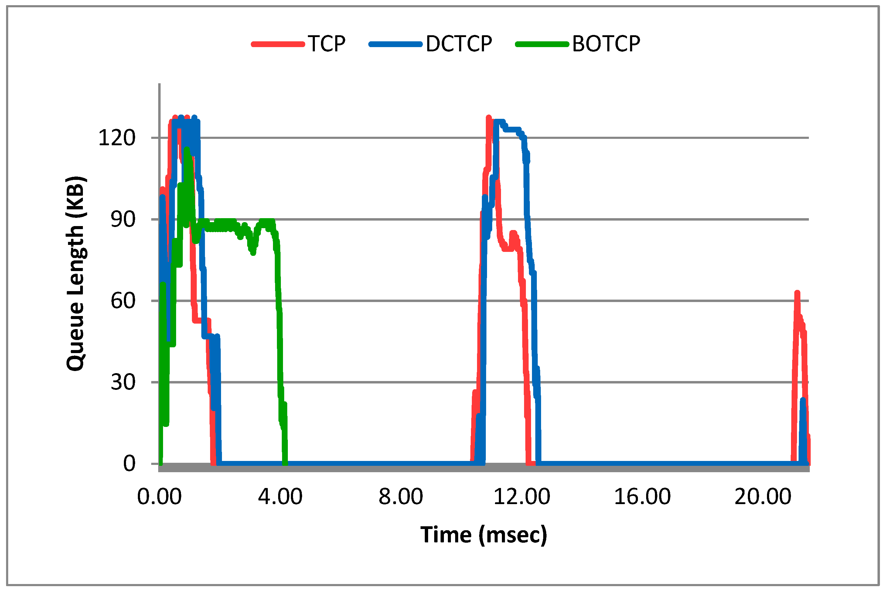
BOTCP quickly transfers the major share of bandwidth from long flows to short flows. This is demonstrated by a specific scenario. In the scenario, at first, two long flows are running through a bottleneck link; then, five new short flows join and share the same bottleneck link. Figure 8 shows the throughput graphs of the long and short flows for the three schemes. As discussed in the previous two sections, in BOTCP, the long flows decrease their congestion windows as ‘MAX (cw × (1 − ((B_cr − B_l)/B_cr), 1)’ and short flows increase their congestion windows as ‘cw × (1 + ((B_s − B_cr)/B_cr))’, in each RTT. Therefore, as shown in Figure 8, the throughput of BOTCP’s short flows gets double in almost every RTT until they finish. Short flows of TCP finish second; this is because TCP reduces the congestion window more drastically than DCTCP when it receives marked ECN bit in ACKs, thereby allowing more bandwidth for new flows. Short flows of DCTCP finish last, this is because DCTCP reduces the congestion window of the existing flows proportional to the fraction of packets marked with ECN bit, thereby allowing lesser bandwidth for new flows. After the short flows finish, the long flows regain all the link capacity.

5.3. Packet Drops

As discussed previously, there are two factors of BOTCP’s better performance than TCP and DCTCP in terms of FCT of short flows. First, priority treatment of short flows; second, minimizing the chances of packet drops. Having the exact information of buffer occupancy at the bottleneck link through its buffer occupancy-based congestion signal (BOF), BOTCP is able to opportunely adjust the sending rates of flows and consequently minimize the chances of packet drops. In comparison, both TCP and DCTCP suffer from packet drops due to an inherently weak congestion signal, the ECN. The ECN mechanism does not indicate the extent of congestion, hence the reaction to moderate and extreme congestions is the same. In addition, both TCP and DCTCP have no solution to the case when the number of flows through the bottleneck link is large enough so that even keeping the congestion window of flows to 1 MSS does not prevent packet drops due to buffer overflow at the bottleneck link; we name this case as ‘extreme flow load’ and discuss it subsequently.

A Case of Extreme Flow Load

Here we discuss a case of how the three congestion control schemes work when put through extreme flow load. Extreme flow load occurs when the number of flows passing through the bottleneck link becomes greater than (buffer capacity at bottleneck link + bandwidth-delay product of the path) divided by MTU. In the scenario, 20 flows, each 50 KB in size, are injected through the same bottleneck link every 200 µsec until the total number of flows through the bottleneck link becomes 100. Figure 9 shows the graph of queue length at the bottleneck link and Figure 10 shows the graph of cumulative distribution function (CDF) of flow completion times. Here, queue length is shown in Kbytes. Since the buffer capacity is 87 packets, the maximum value of queue length is 127 Kb. In BOTCP, when the fourth burst of 20 flows starts, B_cr becomes greater than B_m; BOTCP recognizes this case as extreme flow load and reduces its congestion window below 1 MSS; it then increases or decreases the congestion window using the function (SUB_MSS_CONGESTION_WINDOW) to keep B_cr around B_m until the flow load decreases. Since the constant B_m has the value 60, the queue length is kept around 60 × 1500/1024 ≅ 89 Kb for the duration of the extreme flow load, as shown in the graph of Figure 8. It also gives a burst tolerance of around 27 packets. In comparison, both TCP and DCTCP cannot reduce the congestion window below 1 MSS even when packet drops occur; both schemes retransmit the packet after the timeout occurs. The flows that suffer from packet drop back off for the duration of RTO. The remaining flows continue and finish earlier than in the case of BOTCP, as shown in the CDF of FCT graph in Figure 10; this is because the available capacity is being shared between lesser number of flows, as compared to the case of BOTCP where all hundred flows continue to send data, although with a sending rate of less than 1 MSS. In TCP and DCTCP, the blocked flows resume after the expiry of the RTO at around 11 msec in the graph of Figure 9; again some of the resuming flows suffer from packet drop and back off again for the duration of the RTO and finish after the expiry of the RTO.

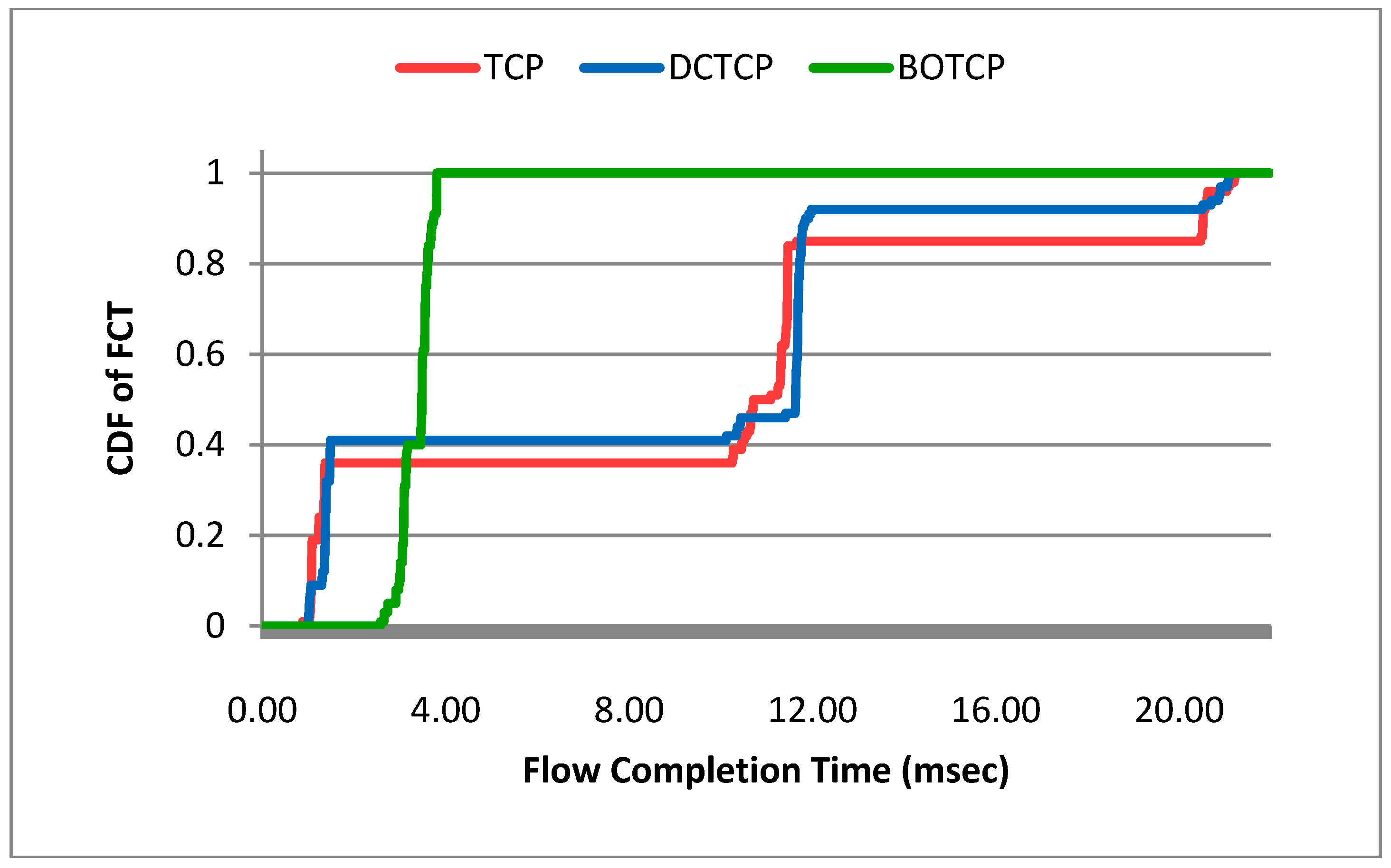
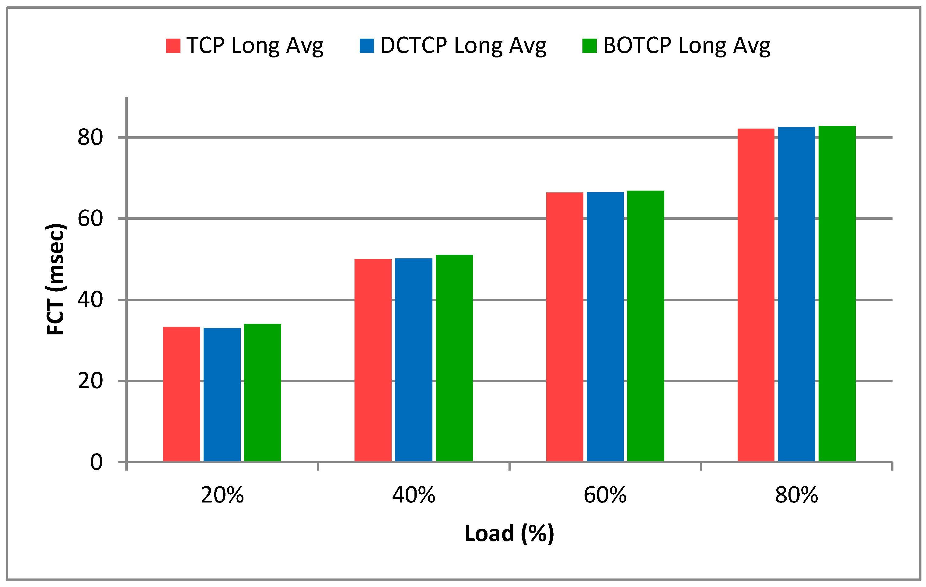
5.4. Flow Completion Time of Long Flows

There is not much difference in the three schemes in terms of average FCT of long flows as shown in the bar chart of Figure 11. This is because long flows remain alive for a much longer period of time compared to short flows, and long flows regain all the available bandwidth when short flows finish. In addition, in TCP and DCTCP, although long flows also experience packet drops, the RTOs (the time period for which the flow is blocked/idle) are much smaller compared to the duration of the flow; therefore, such idle times have no significant effect on the FCT of long flows.

6. Conclusions

In this paper, we presented BOTCP, a buffer occupancy-based transport protocol to reduce flow completion time of short flows. The design objectives of BOTCP are to minimize packet drops, ensure high utilization, and reduce flow completion time of short flows without hurting the overall throughput of long flows. BOTCP consists of two key parts: (i) BOF, a novel congestion signal that gives precise information of congestion along the path from source to destination, and (ii) BOCC, a BOF-based congestion control scheme. The results are compared with TCP and DCTCP, and demonstrate that BOTCP remarkably improves both the average and the 99th percentile of flow completion time of short flows. As a future direction, we aim to modify the congestion control scheme to accommodate flow priorities based on the amount of data transmitted so far.

References

1. Xia, W.; Zhao, P.; Wen, Y.; Xie, H. A survey on data center networking (DCN): infrastructure and operations. IEEE Commun. Surv. Tutor. 2017, 19, 640–656. [Google Scholar] [CrossRef]
2. Abts, D.; Felderman, B. A guided tour of data-center networking. Commun. ACM 2012, 55, 44–51. [Google Scholar] [CrossRef]
3. Hu, J.; Huang, J.; Lv, W.; Zhou, Y.; Wang, J.; He, T. CAPS: Coding-based adaptive packet spraying to reduce flow completion time in data center. In Proceedings of the IEEE INFOCOM Conference on Computer Communications, Honolulu, HI, USA, 15–19 April 2018. [Google Scholar]
4. Liu, S.; Xu, H.; Liu, L.; Bai, W.; Chen, K.; Cai, Z. RepNet: Cutting latency with flow replication in data center networks. IEEE Trans. Serv. Comput. 2018. [Google Scholar] [CrossRef]
5. Ousterhout, J.; Agrawal, P.; Erickson, D.; Kozyrakis, C.; Leverich, J.; Mazières, D.; Rumble, S.M. The case for RAMClouds: Scalable high-performance storage entirely in DRAM. ACM SIGOPS. Oper. Sys. Rev. 2010, 43, 92–105. [Google Scholar] [CrossRef]
6. Guo, C.; Wu, H.; Tan, K.; Shi, L.; Zhang, Y.; Lu, S. Dcell: A scalable and fault-tolerant network structure for data centers. ACM SIGCOMM Comput. Commu. Rev. 2008, 38, 75–86. [Google Scholar] [CrossRef]
7. Zhang, Y.; Ansari, N. On architecture design, congestion notification, TCP incast and power consumption in data centers. IEEE Commun. Surv. Tutor 2013, 15, 39–64. [Google Scholar] [CrossRef]
8. Al-Tarazi, M.; Chang, J.M. Performance-aware energy saving for data center networks. IEEE Trans. Netw. Serv. Manag. 2019, 16, 206–219. [Google Scholar] [CrossRef]
9. Zhang, J.; Ren, F.; Lin, C. Survey on transport control in data center networks. IEEE Netw. 2013, 27, 22–26. [Google Scholar] [CrossRef]
10. Huang, J.; Lv, W.; Li, W.; Wang, J.; He, T. QDAPS: Queueing delay aware packet spraying for load balancing in data center. In Proceedings of the IEEE 26th International Conference on Network Protocols, Cambridge, UK, 24–27 September 2018. [Google Scholar]
11. Sreekumari, P.; Jung, J. Transport protocols for data center networks: A survey of issues, solutions and challenges. Photonic Netw. Commun. 2016, 31, 112–128. [Google Scholar] [CrossRef]
12. Kandula, S.; Sengupta, S.; Greenberg, A.; Patel, P.; Chaiken, R. The nature of data center traffic: Measurements & analysis. In Proceedings of the 9th ACM SIGCOMM Conference on Internet Measurement, Chicago, IL, USA, 4–6 November 2009. [Google Scholar]
13. Greenberg, A.; Hamilton, J.R.; Jain, N.; Kandula, S.; Kim, C.; Lahiri, P.; Sengupta, S. VL2: A scalable and flexible data center network. ACM SIGCOMM Comput. Commu. Rev. 2009, 39, 51–62. [Google Scholar] [CrossRef]
14. Benson, T.; Anand, A.; Akella, A.; Zhang, M. Understanding data center traffic characteristics. ACM SIGCOMM Comput. Commun. Rev. 2010, 40, 92–99. [Google Scholar] [CrossRef]
15. Ren, Y.; Zhao, Y.; Liu, P.; Dou, K.; Li, J. A survey on TCP Incast in data center networks. Int. J. Commun. Syst. 2014, 27, 1160–1172. [Google Scholar] [CrossRef]
16. Zeng, G.; Bai, W.; Chen, G.; Chen, K.; Han, D.; Zhu, Y. Combining ECN and RTT for datacenter transport. In Proceedings of the First Asia-Pacific Workshop on Networking, Hong Kong, China, 3–4 August 2017. [Google Scholar]
17. Shan, D.; Ren, F. Improving ECN marking scheme with micro-burst traffic in data center networks. In Proceedings of the IEEE INFOCOM Conference on Computer Communications, Atlanta, GA, USA, 1–4 May 2017. [Google Scholar]
18. Chen, Y.; Griffith, R.; Liu, J.; Katz, R.H.; Joseph, A.D. Understanding TCP incast throughput collapse in datacenter networks. In Proceedings of the 1st ACM Workshop on Research on Enterprise Networking, Barcelona, Spain, 21–21 August 2009. [Google Scholar]
19. Shukla, S.; Chan, S.; Tam, A.S.-W.; Gupta, A.; Xu, A.; Chao, H.J. TCP PLATO: Packet labelling to alleviate time-out. IEEE J. Sel. Areas Commun. 2014, 32, 65–76. [Google Scholar] [CrossRef]
20. Zhang, J.; Ren, F.; Yue, X.; Shu, R.; Lin, C. Sharing bandwidth by allocating switch buffer in data center networks. IEEE J. Sel. Areas Commun. 2014, 32, 39–51. [Google Scholar] [CrossRef]
21. Zhang, J.; Ren, F.; Shu, R.; Cheng, P. TFC: Token flow control in data center networks. In Proceedings of the Eleventh European Conference on Computer Systems, London, UK, 18–21 April 2016. [Google Scholar]
22. Pal, M.; Medhi, N. VolvoxDC: A new scalable data center network architecture. In Proceedings of the Conference on Information Networking, Chiang Mai, Thailand, 10–12 January 2018. [Google Scholar]
23. Alvarez-Horcajo, J.; Lopez-Pajares, D.; Martinez-Yelmo, I.; Carral, J.A.; Arco, J.M. Improving Multipath Routing of TCP Flows by Network Exploration. IEEE Access 2019, 7, 13608–13621. [Google Scholar] [CrossRef]
24. Zhang, J.; Yu, F.R.; Wang, S.; Huang, T.; Liu, Z.; Liu, Y. Load balancing in data center networks: A survey. IEEE Commu. Surv. Tutor. 2018, 20, 2324–2352. [Google Scholar] [CrossRef]
25. Wang, P.; Trimponias, G.; Xu, H.; Geng, Y. Luopan: Sampling-based load balancing in data center networks. IEEE Trans. Parallel Distrib. Syst. 2019, 30, 133–145. [Google Scholar] [CrossRef]
26. Ye, J.L.; Chen, C.; Chu, Y.H. A Weighted ECMP Load Balancing Scheme for Data Centers Using P4 Switches. In Proceedings of the IEEE 7th International Conference on Cloud Networking (CloudNet), Tokyo, Japan, 22–24 October 2018. [Google Scholar]
27. Munir, A.; Qazi, I.A.; Uzmi, Z.A.; Mushtaq, A.; Ismail, S.N.; Iqbal, M.S.; Khan, B. Minimizing flow completion times in data centers. In Proceedings of the IEEE INFOCOM, Turin, Italy, 14–19 April 2013. [Google Scholar]
28. Alizadeh, M.; Greenberg, A.; Maltz, D.A.; Padhye, J.; Patel, P.; Prabhakar, B.; Sridharan, M. Data center tcp (dctcp). ACM SIGCOMM Compu. Commu. Rev. 2011, 41, 63–74. [Google Scholar]
Figure 1. A scenario of available capacity usage by short and long flows.
Symmetry 11 00646 g001
Figure 2. Explicit congestion notification (ECN) marking mechanism, (a) if queue is empty, the ECN bit is set to 0, (b) if queue length is just below the threshold (K), the ECN bit is set to 0, (c) if queue length is just above the threshold (K), the ECN bit is set to 1, (d) if queue is full, the ECN bit is set to 1.
Symmetry 11 00646 g002
Figure 3. An illustration of how the short and long flows increase and decrease their sending rates, respectively, to bring the Bcr to their respective allowed buffer occupancy limits.
Symmetry 11 00646 g003
Figure 4. A pictorial view of interaction between transport layer and IP protocols; Oct 1 and Oct 2 represent the first and second octet of buffer-occupancy-feedback option-data, respectively; when IP receives a packet from the network it hands-over the payload and the two octets to the upper layer; the value in the second octet is used by the transport entity in its congestion control scheme and the first octet is echoed back (as the second octet over the reverse path) to the other end of the connection.
Symmetry 11 00646 g004
Figure 5. Process of collecting the buffer occupancy feedback (BOF) at a switch.
Symmetry 11 00646 g005
Figure 6. Graph of average FCT of short flows.
Symmetry 11 00646 g006
Figure 7. Graph of 99th percentile of flow completion time (FCT) of short flows.
Symmetry 11 00646 g007
Figure 8. Throughput graph of a scenario of long/short flows for each of the three schemes one above the other.
Symmetry 11 00646 g008
Figure 9. Graph of queue length at bottleneck link in extreme flow load scenario.
Symmetry 11 00646 g009
Figure 10. Graph of CDF of FCTs in extreme flow load scenario.
Symmetry 11 00646 g010
Figure 11. Bar chart of average FCT of long flows.
Symmetry 11 00646 g011