Article

Improved Sparse Coding Algorithm with Device-Free Localization Technique for Intrusion Detection and Monitoring

1
School of Computer Science and Engineering, University of Aizu, Aizu-Wakamatsu, Fukushima 965-0006, Japan
2
School of Artificial Intelligence, Guilin University of Electronic Technology, Guilin 541004, China
*
Authors to whom correspondence should be addressed.
Symmetry 2019, 11(5), 637; https://doi.org/10.3390/sym11050637
Submission received: 3 April 2019 / Revised: 23 April 2019 / Accepted: 24 April 2019 / Published: 6 May 2019

Abstract

:
Device-free localization (DFL) locates target in a wireless sensors network (WSN) without equipping with wireless devices or tags, which is an emerging technology in the fields of intrusion detection and monitoring. In order to achieve an accurate result of DFL, the conventional works adopt l 1 norm as a regularizer to take the full potential of sparsity for locating targets. Contrasting to the previous works, we exploit the l 2 , 1 norm as the regularizer and devise an efficient optimization method with a proximal operator-based scheme, which leads the proposed improved-sparse-coding algorithm with proximal operator (ISCPO). Compared with the state-of-the-art methods that adopt l 1 norm as the regularizer, the proposed algorithm can improve the joint sparsity of sparse solution. Experimental results on our real testbeds of indoor DFL show that, in scenarios of living room and corridor, the proposed approach can achieve high localization accuracies of about 100% and 90%, respectively. In addition, the proposed ISCPO algorithm outperforms the compared state-of-the-art methods and has a more robust performance in challenged environments for target localization.

1. Introduction

In recent years, wireless technologies have attracted tremendous attentions in the field of security safeguard [1,2]. Device-free localization (DFL) [3], using wireless sensor networks (WSNs) to locate targets without carrying any attached devices or tags, has been an emerging technique for some emerging scenarios, e.g., intrusion detection and monitoring [4,5]. This looks impossible but has been shown realizable. As shown in Figure 1, the fundamental blocks of Internet-of-Things (IoT) networks with DFL system are presented in detail. WSNs are utilized to sense data on the target’s location-information in the DFL system and then the sensed data are sent to the edge server for processing. After data processing, the location-information can be mined for user access. As in the description of Figure 1, the user can be a doctor or a guardian for aging healthcare, security personnel or a house host for security safeguards, a manager for the location services of a shopping center, etc. Thus, the DFL model can be applied to the IoT-based applications as described at the beginning of Section 1.
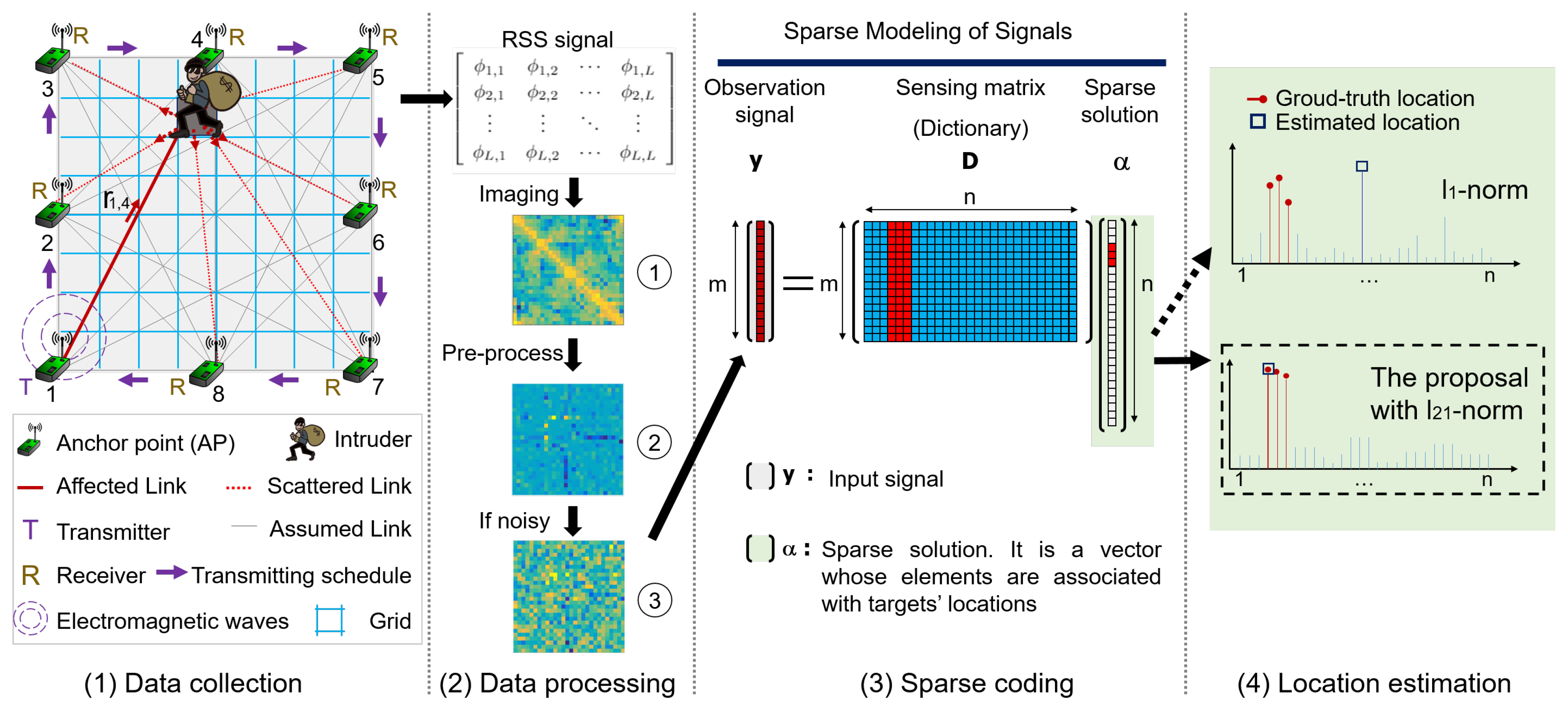
For an easy understanding, a monitoring system with DFL is illustrated in step (1) of Figure 2. In this DFL system, the monitoring area is discretized into a number of grids. Meanwhile, wireless sensor nodes, normally termed as anchor points (APs), are deployed for sensing the signals collaboratively by transmitting and receiving wireless signals. When a person appears at one of these grids, it can attenuate the energy of signal broadcasting. Moreover, this will lead to the variations of these transmitting-receiving correspondences when the target locates at different positions. That is, the sensed signals may conceal location information of targets.
Since APs will generate the sensed data with a pattern, i.e., feature, differently associated with the target’s location, the pattern information can be collected for the localization processing. From this point of view, the previous works have reported that the localization problem can be transferred to a classification problem. In addition, like step (2) of Figure 2, if the sensed data are processed through our pre-process (Detailed procedure will be given in Section 3.2.1), the useful pattern information with a distinguished characteristic can be mined. In consequence, the target’s location can be estimated by many popular classification methods, such as deep learning [6], support vector machine (SVM) [7], K-nearest-neighbor (KNN) [8] and so on.
Among these various classification methods, the sparse coding algorithm [9] is exploited based on the theory of sparse representation. Then, it is famous in the DFL field for several distinctive advantages, including high accuracy, high efficiency, simple operation and its ability to locate multi-targets etc. According to our previous work [10], the sparse coding algorithm with l 1 norm can achieve better localization performance than several classification methods, e.g., deep auto-encoder, KNN, etc. More specifically, the localization problem can be transformed into a typical sparse-representation-classification (SRC) problem, which can be effectively solved by sparse coding [10]. In step (3) of Figure 2, the overall framework and the basic principle of sparse coding is illustrated. It can be seen that, when an observation signal inputs the sparse model, through sparse coding, the sparse solution is obtained. Since the elements of sparse solution associated with the target’s location are outstandingly nonzero, then in step (4), the target’s locations can be estimated.
It is worth noting that the objective function of an SRC problem usually consists of two terms, i.e., loss and regularizer. Employing a different regularizer can drive a different type of sparse coding algorithm. During the various kinds of regularizers [11,12,13], the most famous regularizers are l 1 norm and have been popularly employed in many DFL related works [10,14]. Usually, since the elements’ indices of sparse solution are associated with the grids’ ID, the target is located by selecting the maximum in a sparse solution while the l 1 norm is used as the regularizer. These algorithms are simple and effective for locating targets with high accuracy in the noiseless case.
Generally, for most of the localization experiments in existing DFL-related works, the sensing data are usually collected from wireless sensors in a static or clean environment. This may make their methods achieve the relatively accurate localization results. However, in the practical application, the monitoring environment may be challenged, such as the vibration of transceivers caused by wind, or electromagnetic interference caused by surrounding wireless devices in indoor or outdoor DFL. These adverse conditions will result in the DFL signals collected with various levels of noises. In this case, DFL data may be polluted, like the case of step (2) in Figure 2, which will lead to a serious adverse effect on target localization. Therefore, a robust DFL algorithm is necessary for working in the extreme environments.
Normally, the sparse-based DFL approach consists of two stages, i.e., an offline stage for constructing the sensing matrix and an online stage for estimating targets’ locations based on the so-called sensing matrix. The offline stage includes step (1) and (2) of Figure 2 while the online locating stage contains from step (1) to step (4). (The processes of these two stages are presented in the following Section 3.2.2 in detail).
Since, in the offline stage, multiple samples are collected, for robustness, when an obstacle is at each grid, and then they are stacked into the sensing matrix, there are multiple columns associated with one grid, i.e., one reference position. That is to say, in step (3) and (4) of locating targets with sparse coding, one target’s location is corresponding to multiple elements of the sparse solution, i.e., a group of elements. For example, as illustrated in the step (4) of Figure 2, the outstanding non-zero elements marked with the red stems are corresponding to the target’s ground-truth location.
As mentioned above, employing different regularizers leads to different sparse patterns. Usually, l 1 norm regularizer generates the element-wise sparsity because it regards each element as a singleton and generates the sparse codes independently. Whereas, due to the adverse of serious noise, there may exist another element with a larger non-zero value, for example, the element marked with a blue-square stem in step (4) of Figure 2. In this case, if the l 1 norm is employed for DFL, the target could be located at an incorrect grid.
Contrasting to the related works [14,15] and our previous work [10] on employing l 1 norm, in this paper, we proposed to exploit the new regularizer via l 2 , 1 norm for measuring the block-sparsity, so that the DFL algorithm can achieve a robust process in the challenging environments. That is, the collected multiple samples are considered as one group in the sensing matrix when an obstacle is at each grid. Then the l 2 , 1 norm is used for measuring group sparsity of the coefficent vector. For a clear comparison, we list the difference in Table 1. From the comparisons of Table 1 and the illustration of step (4) in Figure 2, the l 2 , 1 norm regularizer generates a group sparsity. That is, the whole group of elements are jointed in each class for improving the joint sparsity, which leads the proposed improved sparse coding algorithm. Obviously, the l 2 , 1 norm regularizer takes the natural group structure of a sample into account and is expected to achieve a better sparse representation performance than l 1 norm. However, since the l 2 , 1 norm regularizer is non-differentiable in some places and is more complicated than l 1 norm, the problem is not straightforwardly solvable. For this, we exploit the proximal operator method that is effective for solving the non-smooth convex optimization problem in the proposed algorithm. Then, through the proposed improved sparse coding with proximal operator (ISCPO) algorithm, we further use the improved sparse solution for locating target, which is expected to achieve more accurate localization results and a robust localization performance.
The major contributions of this article can be summarized as follows:
  • This paper proposes a block-group regularizer to extend the theory of the previous sparse-representation-based frameworks for DFL.
  • We propose an improved sparse coding algorithm to achieve the robust DFL. Especially, through a modification on the objective function, we exploit the effective optimization process with the proximal operator for localizing target.
  • For evaluating the localization performance and robustness of the proposed method, we establish the testbeds of indoor DFL system. Our experimental results show that the proposed method is more effective than the state-of-the-art sparse coding algorithms for DFL, especially in noisy cases.
The remainder of this paper is organized as follows. Section 2 gives an overview of the related works. Section 3 introduces the system model and problem formulation. The design of objective function and the proposed algorithm are presented in Section 4. Section 5 demonstrates the experimental results of performance evaluation. Finally, Section 6 concludes the whole work.

2. Related Work

Based on the WSNs and classification mechanism, many methods have been exploited for indoor or outdoor localization in the past studies [6,18]. The relevant literature is briefly summarized in this section.
Zhang et al. [19] utilized a compressive-sensing (CS) based method for solving the problems of sparse target counting and locating with wireless sensor networks. They proposed a greedy matching pursuit algorithm that could correctly count and locate targets from a small number of measurements. Wang et al. [16,20] applied a CS based model and used a Bayesian greedy matching pursuit algorithm to locate the target. Wang et al. [17] focused on the sparse representation theory for locating single-target and utilized the CVX tool that solved the basis pursuit problem via linear programming. Whereas, according to our previous work [10,21], CVX tool could not apply to the real-time detecting targets because it was very inefficient for the high dimensional data. Feng et al. [22] applied the sparse model in an RSS-based indoor positioning system, which recovered sparse signals from a small set of noisy measurements through solving the l 1 -minimization problem. Zhao et al. [6,23] utilized the deep neural network with auto-encoder for outdoor DFL. In our previous work [10], the l 1 norm-based sparse coding algorithms presented higher localization accuracy than the deep auto-encoder neural network.
For this sparsity-based DFL research, the objection functions are usually comprised of two parts as follows:
J ( α ) = argmin α Loss + Regularizer
where the loss term is used to achieve the minimum reconstruction error [10,24] between observed signal and estimated signal, regularizer [12,25] is usually used to generate the sparsity of the solution, and α is called sparse solution that can be used to estimate targets’ locations [10]. Considering the sparse distribution of targets in the monitoring area, the more sparse a solution is, the more accurate its localization will be. For the process of sparse coding, different regularizer will generate different sparse patterns. For example, the previous studies [15,24] employ l 1 norm as the sparsity regularizer, which will derive a good element-wise sparsity in the solution. That is, l 1 norm considers each element independently and generates the sparse codes through element by element. However, the prior of targets’ sparse distribution has not been fully utilized because one target’s location is associated with a group of elements.
Contrasting with the above works, in order to obtain a robust DFL algorithm, we exploit the block-sparsity regularizer via l 2 , 1 norm. The block-sparsity regularizer will take the sparsity in the whole group of elements into account and generate the jointly sparse pattern in the sparse solution. Therefore, the proposed approach will make full use of the sparse feature for target localization, which is expected to achieve more accurate localization results and robust performance compared with the previous l 1 norm-based sparse coding algorithm. For clear comparison, we present the difference between the proposed approach and the previous works, e.g., [10,16,17], in Table 1. Moreover, since the l 2 , 1 norm regularizer is non-differentiable in some cases, it will be hard to solve by the conventional optimization methods. To address this problem, in the proposed improved sparse coding algorithm, we exploit a proximal operator method that is effective for solving the non-smooth optimization problem.

3. Problem Formulation

In this section, we will first describe the procedure of background elimination for DFL data, followed by transforming the DFL problem into a sparse-representation-based image classification problem, and finally, present the sparse model.

3.1. Preliminary on System Model

As shown in the above-mentioned step (1) of Figure 2, for more accessibility to the problem, the monitoring area is discretized into grids and is surrounded by several wireless APs (i.e., transmitter-receivers). A target can disturb signal broadcasting because of absorbing, diffracting and scattering, which will change the values of the received signal strength (RSS) measurements at APs. Then, different joint signal configurations consisting of RSS measurements will be collected when the target is at different grids. Besides, RSS matrices obtained from the same target’s location will indicate similar features. Therefore, if each grid captured by the target is viewed as a class, the localization problem can be transformed into a classification problem.
Furthermore, we treat each signal measurement as an image-pixel and image the RSS matrix. Then, an RSS image with a special pattern is obtained, for example, the image ① shown in step (2) of Figure 2. Since the measured RSS signal is much stronger than the variation caused by the target, some important features are submerged in the original RSS measurements, which leads to an adverse effect for locating the target. To weaken this adverse effect, by performing a process of background elimination, a clear image with the distinguished features can be obtained, as shown in the image ② of Figure 2. If the target is shifted from one grid to another, we can obtain the variation image with respective features. As a result, the localization problem can be well formulated with the sparse representation model and be effectively solved through the proposed improved sparse coding algorithm.
In the following subsections, we will describe the principle and the process of sparse representation for DFL in detail.

3.2. Sparse Representation Model of DFL

In this subsection, the procedure of developing the sparse representation model of DFL is presented, including data collection and process, dataset construction, sparse representation of a testing signal and introducing the related objective function.

3.2.1. Data Collection and Process of Background Elimination

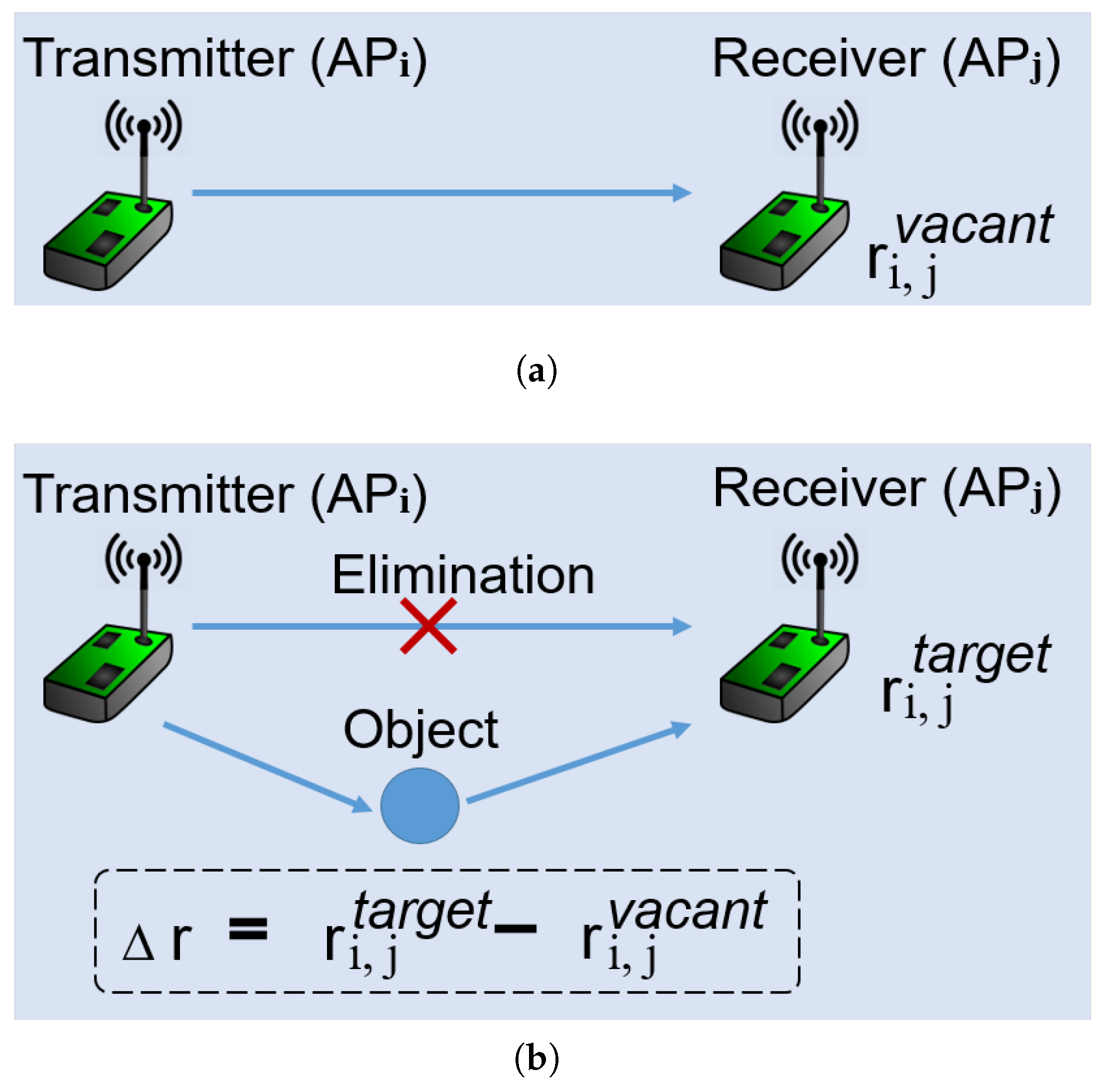
Here, we let r i , j denote the RSS measurement from the i-th AP to the j-th AP while a target is at a known grid, as shown in Figure 3; r i , j vacant denote the RSS measurement collected in the vacant monitoring area, i.e., a vacant area; let r i , j target denote the measurement with a target existing in the monitoring area. Then, the background elimination can be conducted as
Δ r i , j = r i , j target r i , j vacant
where Δ r i , j denotes the variation of RSS measurement caused by target. The process is illustrated in Figure 3. After this process, the signal component from the static environment can be eliminated and the signal variation will be distinguished.
Suppose that the total number of all APs is N and all APs are transmitter-receivers. As shown in step (1) of Figure 2, each AP works as a transmitter according to a time-schedule whereas the others receive and measure the signal. Then, when one entire schedule is finished, the matrix Δ R , considering the variations of all N APs, can be established as follows:
Δ R = Δ r 1 , 1 Δ r 1 , 2 Δ r 1 , N Δ r 2 , 1 Δ r 2 , 2 Δ r 2 , N Δ r N , 1 Δ r N , 2 Δ r N , N

3.2.2. Dataset Construction

There are two steps for dataset construction:
Offline stage for constructing sensing matrix (dictionary). Assume that the monitoring area is discretized into C grids as shown in Figure 2, and each grid is regarded as one location i.e., one class. Therefore, all the potential locations are divided into C classes in this DFL problem. For each class c = 1 , 2 , , C , we perform experiments of l = 1 , , L trials with an object at this grid. For each trial, through data collection and background elimination, we can get an variation matrix data, Δ R c l R N × N . Then, we convert the variation matrix Δ R c l to a variation vector d c l by merging all the columns into the vector. Finally, stacking all the variation vectors together, we can obtain the sensing matrix with location information for all grids and trials as D = [ d 11 , d 12 , d 1 L , , d c 1 , , d c L , , d C 1 , , d C L ] . This sensing matrix D is normally termed as dictionary, with a size of m × n . For m = N 2 , n = C L .
Online stage for processing the test signal. In the online test step, the same procedure is taken for processing the observation signal. Then, we can obtain the vector of observation signal as y when M targets separately locate at several certain grids, where M must be smaller than the number of total grids. If M = 1, it is a single-target localization task; If M > 1, it is a multi-target localization problem.

3.2.3. Sparse Representation of Testing Signal

From Section 3.1, we know that the localization problem can be transformed into a classification problem. In this part, we will further formulate it as a sparse representation based classification problem. The idea is derived from the model of sparse representation based image classification [24].
According to the last part in Section 3.2.2, in the online testing step, when targets enter into the monitoring area, a (testing) observation signal y will be obtained. Suppose that the target is close to the p-th grid. Which means that target belongs to the p-th class. If sufficient samples are given, i.e., conducting enough trials at the p-th grid in the offline stage, the testing signal y can be linearly represented with the two corresponding sample-sets of dictionary D . The linear representation is given as follows:
y = D α + e l = 1 L d p l α p l for 1 < p < C
where α = [ 0 0 α p 1 α p L 0 0 ] T R n is a vector comprised of coefficients; α p j R (for 1 < j < L ) are the non-zero coefficients belonging to the p-th class; e indicates the noise.
In summary, due to the sparse nature of DFL, the number of targets’ locations is far smaller than all grids of the monitoring area, the linear representation of observation signal y can be sparsely represented in terms of n basis samples of the dictionary D . From this point of view, (4) becomes a sparse representation problem for target localization, since α is corresponding to a sparse coefficient vector of which nonzero elements are associated to targets’ locations.

4. Approach

According to the above description, when the target is at a certain grid in the testing step, the observation signal can be sparsely represented with a few basis signals of the related grid. This leads DFL to essentially an SRC problem, that is to say, SRC aims at recovering (or reconstructing) an input signal with a small set of components parsimoniously chosen from an over-complete dictionary, and then classifies the input signal into a class which reaches the minimal reconstruction error.
Hence, the DFL problem can be well formulated with the sparse representation model. Based on the (4), if we can obtain the sparse coefficient vector α , the target location would be known.

4.1. Proposed Solver

4.1.1. Sparse Coding

Sparse coding is the process of computing the sparse solution (i.e., sparse coefficient vector) based on a known dictionary D and the observation signal y . The basic framework of sparse coding is presented in step (3) of Figure 2. It can be seen that, once the sparse solution α is effectively found out, the target will be accurately located. It is worth noting that one target may have several corresponding components in the vector of sparse solution α .
In the practical application, if we want to achieve an accurate or robust DFL, a large number of trials is required in the step of constructing a dictionary. This usually results with a high possibility that the total number of basis samples n is larger than m for the dictionary. Which means that (4) is an undetermined system and its solution is not unique, i.e., the problem is ill-posed.
However, by selecting the sparsest solution, we can make the problem well-posed. This motivates us to solve the optimization problem with the sparsity regularization method to find the sparsest solution. The most popular sparsity regularizers are l 1 norm. However, l 1 norm regularizer regards each element as a singleton. Whereas, due to the adverse of serious noise, the sparse solution of l 1 norm will have some elements with large non-zero values led by the noise, which will result in an incorrect localization result.

4.1.2. Objective Function

In order to find out the sparsest solution, in this article, the proposed approach exploits the l 2 , 1 norm as the sparsity regularizer for solving the DFL problem in challenged environment. The objective function is given as follows:
J ( α ) : α = argmin α 1 2 y D α 2 2 + λ α 2 , 1
where the first term · 2 2 is a measure of fitting error between observation signal and estimated signal; the second term with 2 , 1 norm is sparsity regularizer which generates the group sparsity; λ is a scalable parameter which trades off the fitting error and the sparsity.

4.2. Localization Algorithm with Improved Sparse Coding

According to (5), the l 2 , 1 norm will derive the whole elements of each class being jointed for improving the sparsity, which leads to the proposed improved sparse coding algorithm.

4.2.1. Fundamental Sparse Coding Algorithms via Proximal Operator

Regarding the optimizations of l 0 norm · 0 and l 1 norm · 1 , the normal formulas are given by
P 1 ( v ) : argmin v 1 2 u v 2 2 + γ v 0
P 1 ( v ) : argmin v 1 2 u v 2 2 + γ v 1
Then, the corresponding proximal operators of l 0 norm and l 1 norm are prox · 0 ( · ) and prox · 1 ( · ) , respectively. They are separately given by
prox · 0 ( u i ) = u , | u i | > γ 0 , Otherwise
prox · 1 ( u i ) = u + γ , u i > γ 0 , Otherwise u γ , u i < γ
where u i is the i-th element of vector u .

4.2.2. Improved Sparse Coding Algorithm via Proximal Operator

Since (5) is convex though not smooth, it admits the global optimum. Normally, the sub-gradient method is adopted for solving (5). By incorporating the derivative of (5) to zero, we can obtain the minimizer α as follows,
α = ( D T D + λ ( α 2 , 1 ) α ) 1 D T y
However, processing (10) with sub-gradient method may not be easy. Because, if D is a very large matrix, solving ( D T D ) 1 will result in a high computational cost and take up too much memory.
In this paper, to address this problem, we exploit the proximal operator method for searching the sparse solution. The proximal operator is an efficient method for solving the non-smooth optimization problem. For different objective functions, a specific proximal operator can be derived. Regarding the optimization of non-smooth · 2 , 1 , a normal formula can be given by
P ( v ) : argmin v η u v 2 2 + γ v 2 , 1
In order to coincide with (11), we modify the objective function (5) based on the majorization-minimization (MM) method [26,27], and then transform the problem (5) to an simpler one,
P ( α ) : argmin α μ 2 b α 2 2 + λ α 2 , 1 + K
where K is regarded as a known constant that does not depend on α ; μ is a scaling parameter that should be greater than the largest eigenvalue of ( D T D ), for example, 1.01 times the largest eigenvalue; b is a intermediate variable with the same size of α , given under the following conditions,
b = α ( k ) + 1 μ D T ( y D α ( k ) )
α ( k + 1 ) = prox · 2 , 1 ( b )
where α ( 0 ) = 0 ; prox · 2 , 1 ( · ) is the proximal operator of l 2 , 1 norm, given by
prox · 2 , 1 ( b i ) = ( b i c 2 λ μ ) b i b i c 2 , b i c 2 > λ μ 0 , Otherwise
where b i is the i-th element of b , b i c R L denotes a part of vector b , where is associated with the c-th group containing the element b i .
In summary, we optimize the problem (5) by performing the improved sparse coding via proximal operator. The related proof of the problem transformation is presented in the appendix materials. The optimization process is mainly based on the (13) and (14) in each iteration. Until convergence or the stop rule is satisfied in the k-th iteration, the optimally sparse solution α can be determined as α ( k + 1 ) .

4.2.3. Target Localization Based on the Improved Sparse Solution

From the above analysis, the optimally improved sparse solution α can be obtained by performing (12)–(15). Then we can estimate the target’s locations according to the improved sparse solution α . Here, there are two cases, i.e., single-target localization and multi-target localization. If α includes only one group of non-zero elements, it is a single-target localization problem. If α includes multiple groups of non-zero elements, this means for locating multi-targets. The detailed procedures are given as follows:
Algorithm 1 improved Sparse Coding with Proximal Operator (ISCPO).
Require: y R m , D R m × n , μ , λ , α 0 = 0
Ensure: φ or { φ 1 , , φ S }
 1: for k = 0 to maxiteration do
 2:   b α ( k ) + 1 μ D T ( y D α ( k ) )
 3:   α ( k + 1 ) prox · 2 , 1 ( b )
 4:  Until convergence or reach the maxiteration number.
 5: end for
 6:  α α ( k + 1 )
 7: if Single-target localization then
 8:  Target is located at the φ -th grid according to (16)
 9:   Return φ
 10: end if
Since the elements of sparse solution are associated with the grid, the corresponding grid can be taken as the location of the target. For example, for the total C grids of a monitoring area, the target’s location is estimated at the φ -th grid, where φ is given by
φ = argmax φ { α 11 , , α φ i , , α C L }
As the sparse coding algorithm is based on the improved regularizer, i.e., l 2 , 1 norm, and the proximal operator, the proposed localization algorithm is named as improved sparse coding via proximal operator algorithm (ISCPO).

5. Performance Evaluation

In this section, we evaluate the performance of the proposed approach by building a DFL testbed of indoor monitoring system. All the experiments are performed in MATLABR2016b and executed on a computer of Windows10 64-bit with 8GB RAM and Intel® Core™ i7 CPU.

5.1. Configuration of Experiment

5.1.1. Hardware

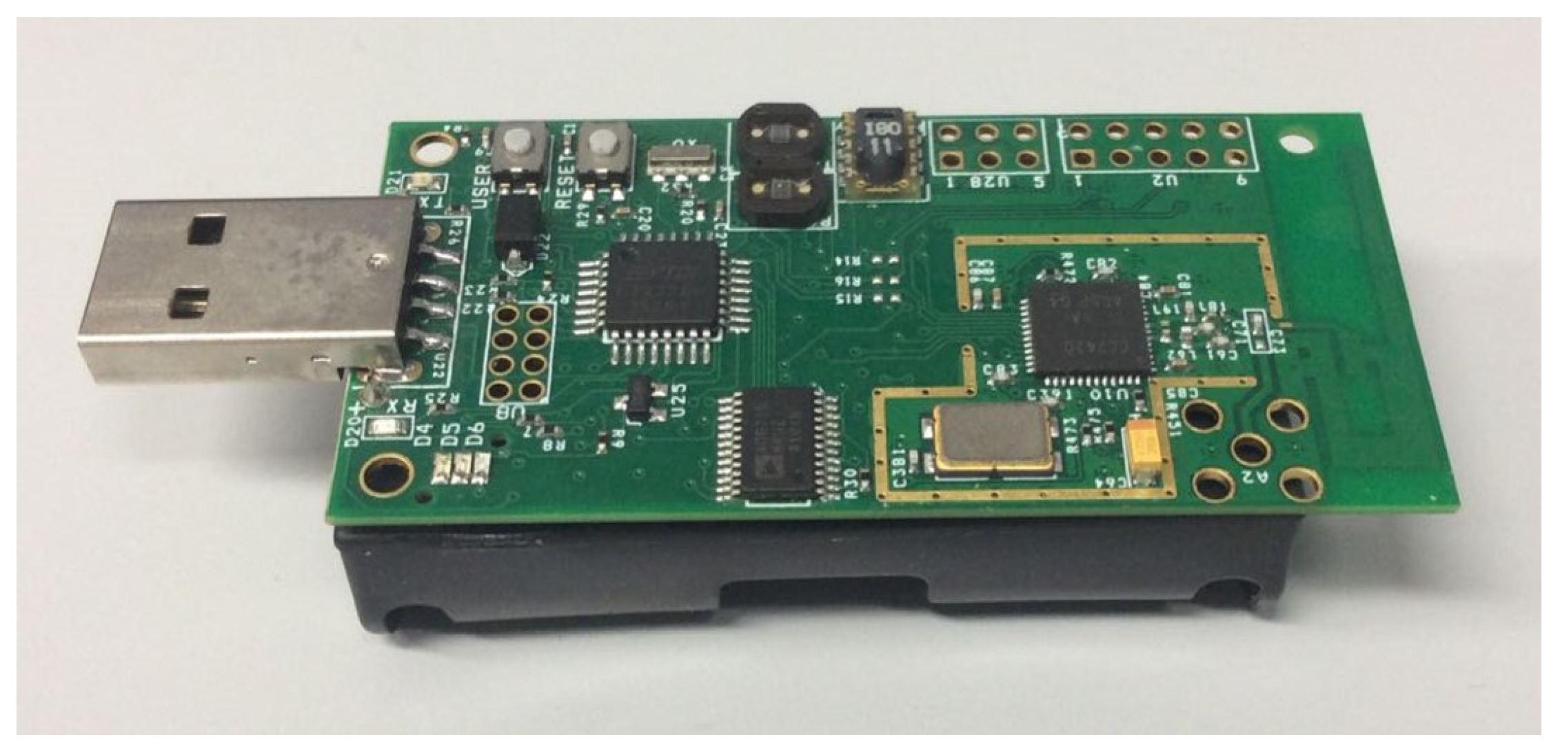
The TelosB wireless sensor node used in indoor DFL, as shown in Figure 4, is made by Crossbow. Each node works in the 2.4 GHz frequency band and uses the IEEE 802.15.4 standard for communication. A base station node listens to the whole network traffic and then delivers the collected data to a computer via a USB port.

5.1.2. Data Pre-Process of Background Elimination

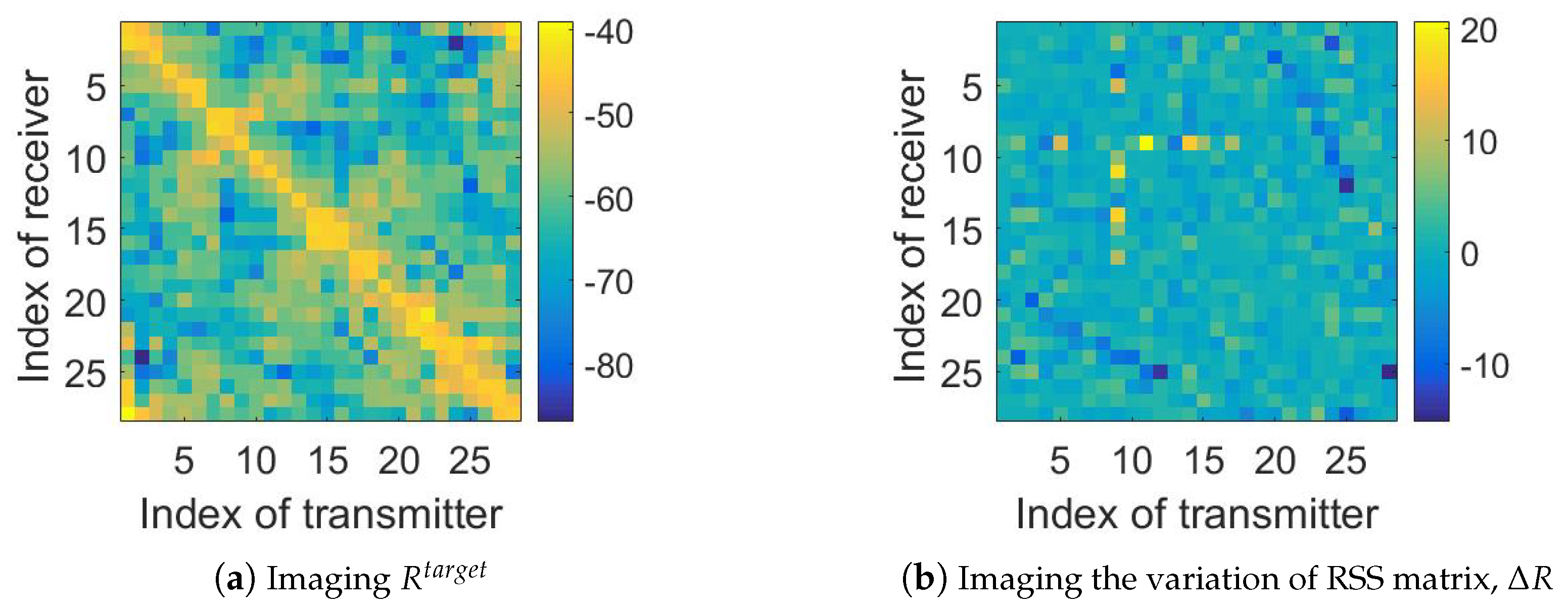
Here, we present an example of processing an outdoor data [23,28] sample, and the process is illustrated in Figure 5. As shown in this figure, since the original RSS signal, with absolute value from 40 dBm to 90 dBm, is measured directly from the environment, it may include many useless signal components which are stronger than the useful signal variation (of which the absolute value is from 0 dBm to 20 dBm). For example, the base signal of the background will not change, no matter if there are targets in the monitoring area. Therefore, a pre-process of background elimination is necessary for DFL data. In the indoor experiments, we perform the data pre-process by subtracting the R v a c a n t from R t a r g e t . Then, after this pre-process, most of the useless signal components can be eliminated and the signal variation will be distinguished.

5.1.3. Compared Approaches

Since l 0 norm and l 1 norm are the most commonly used sparse constraints in the DFL fields, there exist many related references reporting their good effectiveness [10,17,29]. In order to describe the advantages of the proposed ISCPO for DFL, l 0 norm and l 1 norm are the compared methods with respect to localization performance. In addition, for solving the optimization problem with the sparse constraints of l 0 norm and l 1 norm, the most famous sparse-coding-algorithms are OMP and ISTA, respectively.

5.1.4. Other Settings and Metrics

In order to make the presentation clear, the localization accuracy is used as the metrics to evaluate the localization performance of algorithms:
  • Assume that C total is the total number of testing samples and C correct is the number of samples that are correctly located. Then the localization accuracy is defined by
    Accuracy = C correct C total
In practical applications, the DFL system will be disturbed by the environmental noise unavoidably, such as the vibration of transceivers caused by the wind, or electromagnetic interference caused by surrounding wireless devices. Therefore, the robustness is important for a DFL algorithm. In order to evaluate the robustness of the proposed approach under different levels of noises, the additive Gaussian noises are added to the testing signal as well as the dictionary. SNR is used to measure the signal quality under noisy environment.

5.2. Experimental Result of Indoor Localization

In this section, we evaluate the performance of the proposed ISCPO algorithm on our own testbed for indoor DFL. The outline is as follows, (1) introduces the experimental setups of our indoor DFL system, (2) shows the localization performances of the proposed approach and comparisons.

5.2.1. Experimental Setup of Indoor DFL System

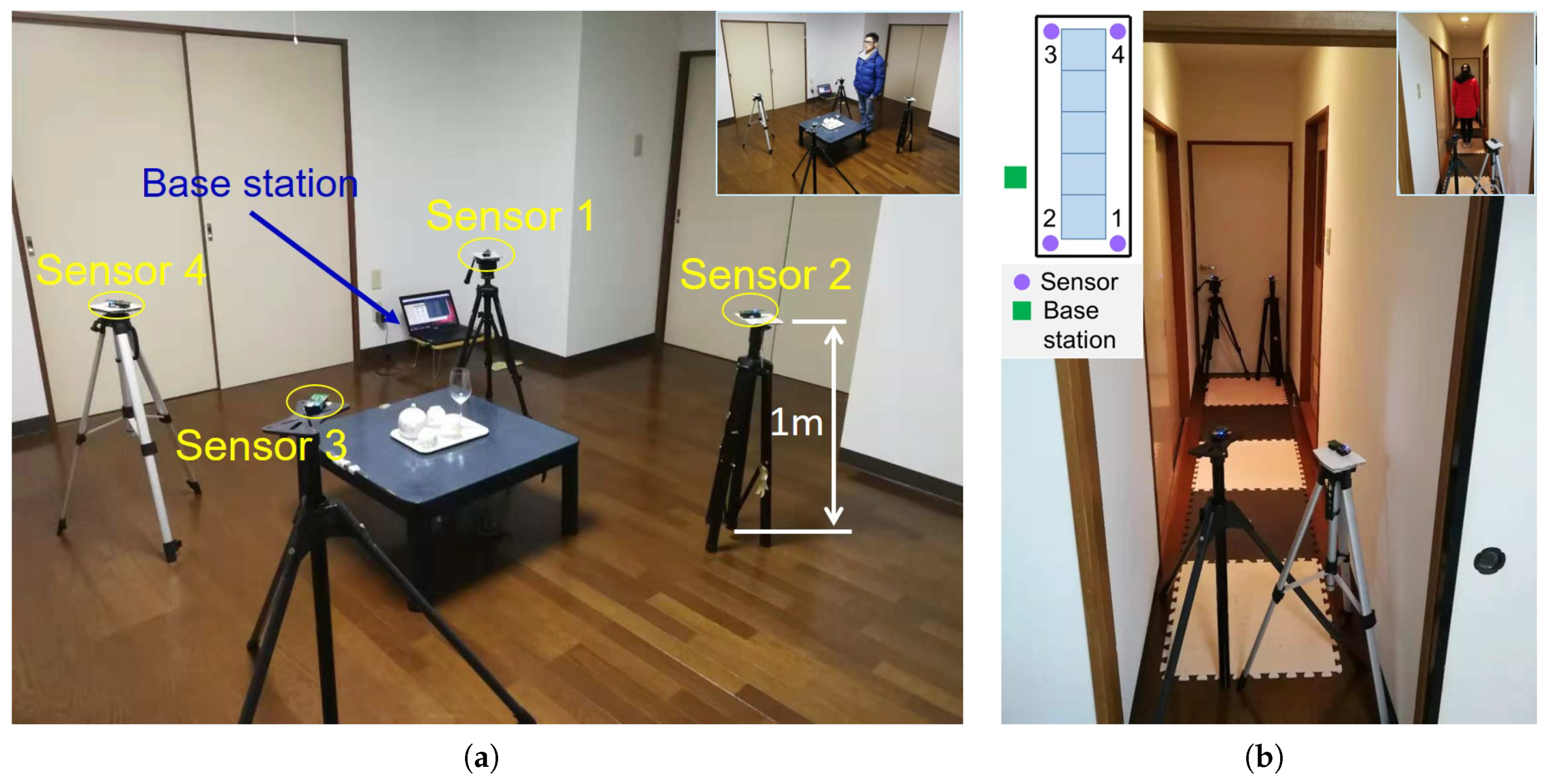
For the indoor DFL, we carry out the experiments in two indoor scenarios, i.e., living room and corridor, respectively. The experimental setups, as shown in Figure 6, have the following settings: Each sensor node is at 1 m off the ground. (1) In the scenario of the living room, 4 TelosB nodes are deployed in a 2.5 × 2.5 m 2 area. Each node is spaced 2 m from the neighbouring nodes. Considering the layout of the room, the validation experiments are performed at 4 positions. The target is a man with the height 1.68 m and the weight 60 kg. (2) In the scenario of the corridor, 4 TelosB nodes are deployed in the 4 corners of the corridor with a 0.8 × 3.5 m 2 area. The target is a girl with a height of 1.60 m and a weight of 49 kg. Then, the dictionary and testing signals are collected in two different steps, respectively.
Dataset descriptions of two scenarios: (1) Scenario of the living room. The data sizes of dictionary and testing signals are 16 × 800 and 16 × 1000, respectively. (2) Scenario of the corridor. The sizes of dictionary and testing signals are 16 × 1250 and 16 × 1000, respectively.
The other processing and settings are the same as the outdoor example, for example, the pre-process of background elimination. Therefore, the final localization results and comparisons will be directly presented in the following content.

5.2.2. Localization Performance of the Proposed Approach and the Comparisons for Indoor DFL

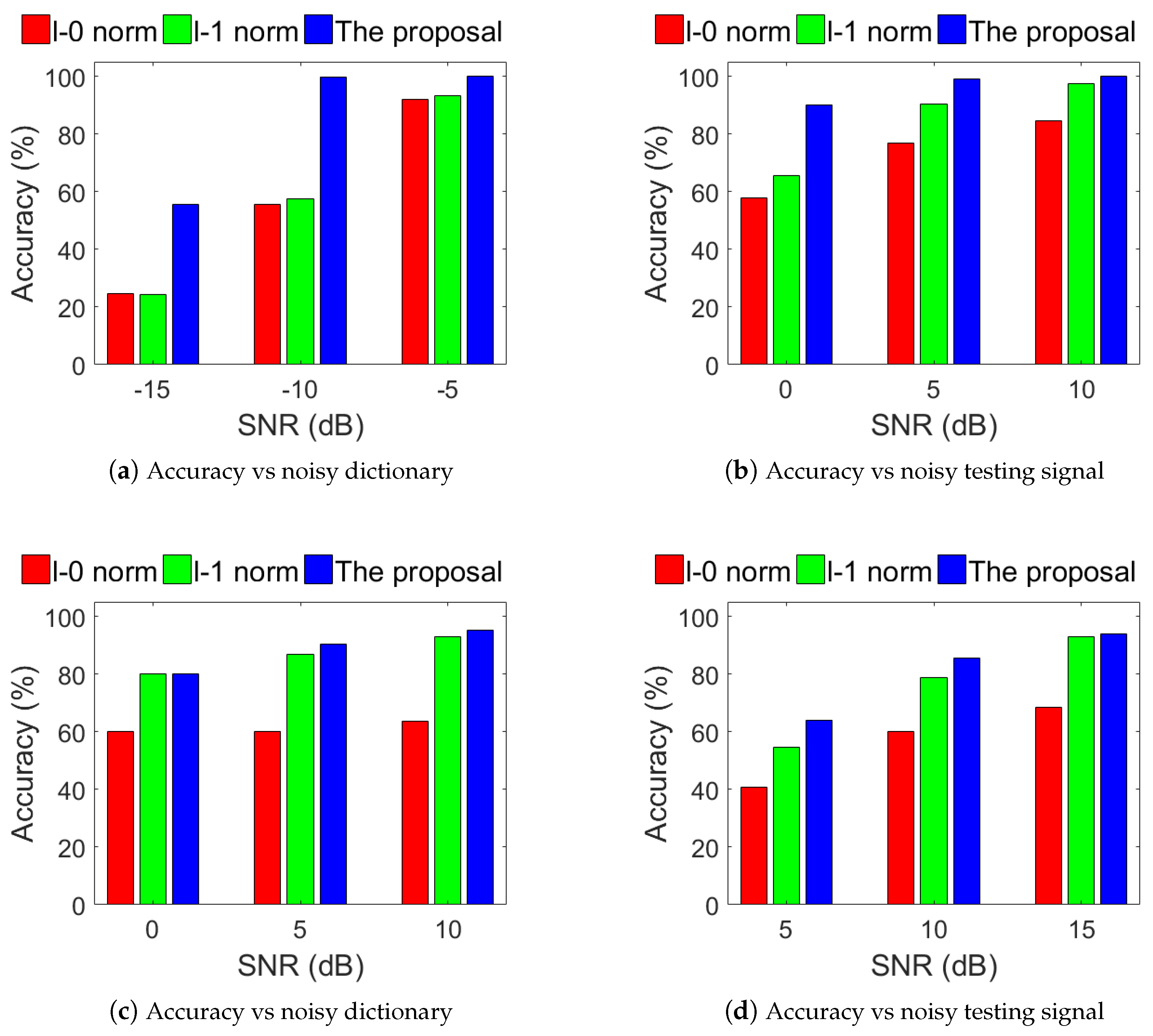
Since the l 2 , 1 norm generates a joint sparsity in the sparse solution, while the l 0 norm and l 1 norm just produce the element-wise sparsity, the localization accuracy and the robustness of l 2 , 1 norm will be better than the other two comparisons. Figure 7 shows the localization results of the proposed approach and comparisons. (a) and (b) are for the scenario of the living room; (c) and (d) are for the scenario of the corridor. It can be seen that the proposed approach outperforms the methods adopted: l 0 norm and l 1 norm, in both of the two scenarios. From Figure 7, in the scenario of the living room, the proposed approach can achieve a high localization accuracy of 100% and is robust to the noisy dictionary with SNR greater than −10 dB (See (a)); the proposed approach also can retain a high accuracy above 90% when SNR of noisy testing signal is greater than 0 dB (See (b)). Then, in the scenario of the corridor, the proposed approach can retain an accuracy of about 90% when SNR of the noisy dictionary is greater than 5 dB or SNR of the noisy testing signal is greater than 15 dB and (See (c) and (d)).

6. Conclusions

In order to achieve an accurate and robust process of DFL, we exploited the l 2 , 1 norm as the regularizer and devised the optimization method with the proximal operator, which led to the proposed improved sparse coding algorithm, ISCPO. Compared with the conventional works that employed l 0 norm or l 1 norm as a regularizer, the proposed approach had the advantage of generating a group sparsity and improving the joint sparsity for the sparse solution.
Experimental results on our real testbeds showed that, in both the indoor DFLs, the proposed approach outperformed the state-of-the-art methods that adopted l 0 norm or l 1 norm as the regularizer. The proposed ISCPO algorithm shows robust performance in the heavy noisy environments for target localization. The main results have been concluded as follows: Indoor DFL experiments. In the scenario of the living room, ISCPO can achieve a high localization accuracy of 100% and is robust to the noisy dictionary with SNR greater than −10 dB (See Figure 7a); ISCPO can remain a high accuracy above 90% when SNR of noisy testing signal is greater than 0 dB (See Figure 7b). Then, in the scenario of corridor, ISCPO can retain an accuracy of about 90% when SNR of the noisy dictionary is greater than 5 dB or SNR of the noisy testing signal is greater than 15 dB and (See Figure 7c,d).

Author Contributions

For this article, formal analysis, H.H., Z.H. and L.Z.; funding acquisition, C.S.; methodology, H.H. and S.D.; project administration, C.S.; supervision, S.D. and C.S.; validation, Z.H. and L.Z.; visualization, Z.H.; writing original draft, H.H.; writing review & editing, S.D.

Funding

This research was funded by the JSPS Kiban(B) (Project number 18H03240) and the JSPS Kiban(C) (Project number 18K11298), Japan, and in part by the National Natural Science Foundation of China (Grant number 61803096). The APC was funded by the JSPS Kiban(B) (Project number 18H03240) and the JSPS Kiban(C) (Project number 18K11298), Japan.

Acknowledgments

The authors thank, Zeyang Dai, Xiang Li, Haoli Zhao, Jianbo Xu and Qinglin Yang for their help in establishing the indoor testbeds as well as Huawei Huang’s comments in revising this paper. The authors sincerely appreciate the valuable comments from the editor and the reviewers, motivating them to further improve this paper.

Conflicts of Interest

The authors declare no conflict of interest.

References

  1. Kolias, C.; Kambourakis, G.; Stavrou, A.; Gritzalis, S. Intrusion detection in 802.11 networks: Empirical evaluation of threats and a public dataset. IEEE Commun. Surv. Tutor. 2016, 18, 184–208. [Google Scholar] [CrossRef]
  2. Kolias, C.; Kambourakis, G.; Maragoudakis, M. Swarm intelligence in intrusion detection: A survey. Comput. Secur. 2011, 30, 625–642. [Google Scholar] [CrossRef]
  3. Kaltiokallio, O.; Yigitler, H.; Jantti, R. A three-state received signal strength model for device-free localization. IEEE Trans. Veh. Technol. 2017, 66, 9226–9240. [Google Scholar] [CrossRef]
  4. Meng, W.; Tischhauser, E.W.; Wang, Q.; Wang, Y.; Han, J. When intrusion detection meets blockchain technology: A review. IEEE Access 2018, 6, 10179–10188. [Google Scholar] [CrossRef]
  5. Meng, W. Intrusion detection in the era of IoT: Building trust via traffic filtering and sampling. Computer 2018, 51, 36–43. [Google Scholar] [CrossRef]
  6. Zhao, L.; Huang, H.; Ding, S.; Li, X. An Accurate and Efficient Device-Free Localization Approach Based on Gaussian Bernoulli Restricted Boltzmann Machine. In Proceedings of the 2018 IEEE International Conference on Systems, Man, and Cybernetics (SMC), Miyazaki, Japan, 7–10 October 2018; pp. 2323–2328. [Google Scholar]
  7. Bisio, I.; Delfino, A.; Lavagetto, F.; Sciarrone, A. Enabling IoT for in-home rehabilitation: Accelerometer signals classification methods for activity and movement recognition. IEEE Internet Things J. 2017, 4, 135–146. [Google Scholar] [CrossRef]
  8. Verma, P.; Sood, S.K. Fog Assisted-IoT Enabled Patient Health Monitoring in Smart Homes. IEEE Internet Things J. 2018, 5, 1789–1796. [Google Scholar] [CrossRef]
  9. Zhao, H.; Ding, S.; Li, X.; Huang, H. Deep Neural Network Structured Sparse Coding for Online Processing. IEEE Access 2018, 6, 74778–74791. [Google Scholar] [CrossRef]
  10. Huang, H.; Zhao, H.; Li, X.; Ding, S.; Zhao, L.; Li, Z. An Accurate and Efficient Device-Free Localization Approach Based on Sparse Coding in Subspace. IEEE Access 2018, 6, 61782–61799. [Google Scholar] [CrossRef]
  11. Han, Y.; Feng, X.C.; Baciu, G.; Wang, W.W. Nonconvex sparse regularizer based speckle noise removal. Pattern Recognit. 2013, 46, 989–1001. [Google Scholar] [CrossRef]
  12. Micchelli, C.A.; Morales, J.M.; Pontil, M. Regularizers for structured sparsity. Adv. Comput. Math. 2013, 38, 455–489. [Google Scholar] [CrossRef]
  13. Li, Z.; Ding, S.; Li, Y.; Yang, Z.; Xie, S.; Chen, W. Manifold optimization-based analysis dictionary learning with an l1/2-norm regularizer. Neural Netw. 2018, 98, 212–222. [Google Scholar] [CrossRef]
  14. Li, X.; Ding, S.; Li, Z.; Tan, B. Device-free localization via dictionary learning with difference of convex programming. IEEE Sens. J. 2017, 17, 5599–5608. [Google Scholar] [CrossRef]
  15. Wang, H.; Leung, C.S.; So, H.C.; Liang, J.; Feng, R.; Han, Z. Robust MIMO Radar Target Localization based on Lagrange Programming Neural Network. arXiv 2018, arXiv:1805.12300. [Google Scholar]
  16. Wang, J.; Gao, Q.; Wang, H.; Cheng, P.; Xin, K. Device-free localization with multidimensional wireless link information. IEEE Trans. Veh. Technol. 2015, 64, 356–366. [Google Scholar] [CrossRef]
  17. Wang, D.; Guo, X.; Zou, Y. Accurate and robust device-free localization approach via sparse representation in presence of noise and outliers. In Proceedings of the IEEE International Conference on Digital Signal Processing (DSP), Beijing, China, 16–18 October 2016; pp. 199–203. [Google Scholar]
  18. Kolias, C.; Kolias, V.; Kambourakis, G. TermID: A distributed swarm intelligence-based approach for wireless intrusion detection. Int. J. Inf. Secur. 2017, 16, 401–416. [Google Scholar] [CrossRef]
  19. Zhang, B.; Cheng, X.; Zhang, N.; Cui, Y.; Li, Y.; Liang, Q. Sparse target counting and localization in sensor networks based on compressive sensing. In Proceedings of the INFOCOM, 2011 Proceedings IEEE, Shanghai, China, 10–15 April 2011; pp. 2255–2263. [Google Scholar]
  20. Wang, J.; Gao, Q.; Wang, H.; Yu, Y.; Jin, M. Time-of-flight-based radio tomography for device free localization. IEEE Trans. Wirel. Commun. 2013, 12, 2355–2365. [Google Scholar] [CrossRef]
  21. Li, Z. Efficient Learning Algorithms for Overcomplete Dictionaries for Sparse Representation of Signal. Ph.D. Thesis, The University of Aizu, Aizu-Wakamatsu, Japan, 2015. [Google Scholar]
  22. Feng, C.; Au, W.S.A.; Valaee, S.; Tan, Z. Received-signal-strength-based indoor positioning using compressive sensing. IEEE Trans. Mob. Comput. 2012, 11, 1983–1993. [Google Scholar] [CrossRef]
  23. Zhao, L.; Huang, H.; Li, X.; Ding, S.; Zhao, H.; Han, Z. An Accurate and Robust Approach of Device-Free Localization with Convolutional Autoencoder. IEEE Internet Things J. 2019. [Google Scholar] [CrossRef]
  24. Wright, J.; Yang, A.Y.; Ganesh, A.; Sastry, S.S.; Ma, Y. Robust face recognition via sparse representation. IEEE Trans. Pattern Anal. Mach. Intell. 2009, 31, 210–227. [Google Scholar] [CrossRef]
  25. Zhu, X.; Li, X.; Zhang, S.; Ju, C.; Wu, X. Robust joint graph sparse coding for unsupervised spectral feature selection. IEEE Trans. Neural Netw. Learn. Syst. 2017, 28, 1263–1275. [Google Scholar] [CrossRef] [PubMed]
  26. Figueiredo, M.A.; Bioucas-Dias, J.M.; Nowak, R.D. Majorization–minimization algorithms for wavelet-based image restoration. IEEE Trans. Image Process. 2007, 16, 2980–2991. [Google Scholar] [CrossRef]
  27. Selesnick, I.W. Sparse Signal Restoration. Available online: http://cnx.org/content/m32168/latest (accessed on 28 April 2019).
  28. Wilson, J.; Patwari, N. Radio tomographic imaging with wireless networks. IEEE Trans. Mob. Comput. 2010, 9, 621–632. [Google Scholar] [CrossRef]
  29. Wang, J.; Zhang, X.; Gao, Q.; Yue, H.; Wang, H. Device-Free Wireless Localization and Activity Recognition: A Deep Learning Approach. IEEE Trans. Veh. Technol. 2017, 66, 6258–6267. [Google Scholar] [CrossRef]
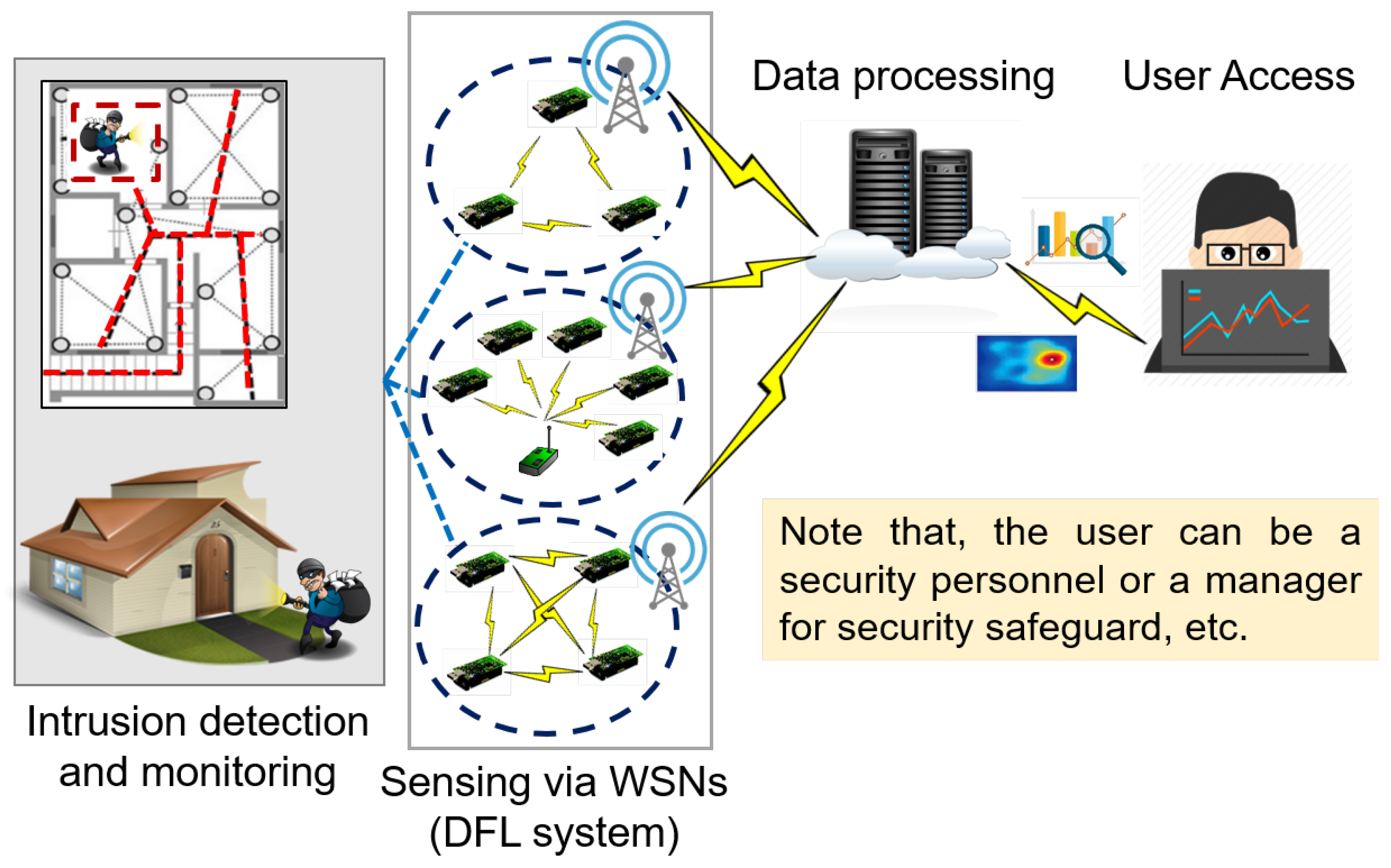
Figure 1. Internet-of-Things (IoT) fundamental blocks with Device-free localization (DFL) system for intrusion detection and monitoring.
Symmetry 11 00637 g001
Figure 2. Illustration for the framework of the proposed device-free localization approach. Here, we show an example of single-target localization. The proposed approach is also applicable to locating multi-targets.
Symmetry 11 00637 g002
Figure 3. Process of background elimination. Here, we take the single-target as an example, but the process is also suitable for the multiple targets. (a) RSS measurement in a vacant monitoring area; (b) RSS measurement and background elimination with a target in monitoring area.
Symmetry 11 00637 g003
Figure 4. TelosB wireless sensor node.
Symmetry 11 00637 g004
Figure 5. Example of data pre-processing by background elimination. Here, the example is randomly selected in which the target is at the 10-th grid. Note that, the variation of (b) is obtained by the signal of (a) subtracting the signal of (Rvacant).
Symmetry 11 00637 g005
Figure 6. Scenarios and experimental setups of indoor DFL system. (a) Scenario of living room; (b) Scenario of corridor.
Symmetry 11 00637 g006
Figure 7. Localization results of the proposed approach and comparisons. (a,b) are for the scenario of living room; (c,d) are for the scenario of corridor.
Symmetry 11 00637 g007
Table 1. Comparisons of the related regularizers.
Compared TermsRegularizerFormulaSparse Pattern
The previous works [10,16,17] l 1 norm α 1 = Σ i = 1 n | α i | 1 Element-wise
The proposed approach l 2 , 1 norm α 2 , 1 = Σ i = 1 g α i 1 2 + + α i c 2 Joint elements (improved sparsity)
Note: α R n is the sparse solution. α can be divided into g group and there are c elements for each group.