Analytical Solutions of Fractional Klein-Gordon and Gas Dynamics Equations, via the (G^′/G)-Expansion Method

Abstract

In this article, the $(G^{{}^{\prime }}/G)$-expansion method is used for the analytical solutions of fractional-order Klein-Gordon and Gas Dynamics equations. The fractional derivatives are defined in the term of Jumarie’s operator. The proposed method is based on certain variable transformation, which transforms the given problems into ordinary differential equations. The solution of resultant ordinary differential equation can be expressed by a polynomial in $(G^{{}^{\prime }}/G)$, where $G=G(\xi )$ satisfies a second order linear ordinary differential equation. In this paper, $(G^{{}^{\prime }}/G)$-expansion method will represent, the travelling wave solutions of fractional-order Klein-Gordon and Gas Dynamics equations in the term of trigonometric, hyperbolic and rational functions.

1. Introduction

The aim of the present paper is to solve the fractional-order a Klein-Gordon and Gas Dynamics equations. In fact, most engineering and physical phenomena are modeled correctly by using fractional Differential Equations (FDEs) [1,2,3]. The FDEs have many applications in science and engineering such as earthquake model [4], signal control system [5], wave models [6], finance models [7] and so on. FDEs have gained much importance among the researchers due to the above mentioned applications. Most of the researchers have presented various techniques for the solutions of FDEs, particularly fractional Partial Differential Equations (FPDEs) is the point of interest.

Among the FPDEs, the Klein-Gordon model is one of the mathematical models in quantum field theory. This model appears in non-linear optics, plasma physics, relativistic physics and also describe dispersive wave phenomena. Moreover, the variety of some other physical phenomena such as ferromagnetic and ferroelectric domain walls, DNA dynamics and Josephson and dislocation junctions are described well by KG model [8].

The gas dynamic(or compressible flow) is a branch of fluid mechanics, which deals with the flow of fluid with significant changes in density. The Gas Dynamic equations explain the behaviour of these compressible flows. These equations are based on physical laws of conservation, namely, laws of conservation of momentum, conservation of mass, conservation of energy and so forth.

In view of the above applications, the mathematicians have developed different numerical and analytical techniques to solve FPDEs [9,10]. For example, J. Song et al. in [11] have applied Fractional Variational Iteration Method (FVIM) for the solutions of some FPDEs. Duan et al. have used Adoman’s Decomposition Method (ADM) to obtain series form solutions of different Partial Differential Equations (PDEs) and FPDEs with initial and boundary conditions [12]. Similarly, in [13] Rasool Shah et al. have applied Laplace ADM for solving a system of FPDEs. Homotopy Perturbation Method (HPM) has been applied by Wang for solving fractional kdV-Burger equations numerically [14]. With the help of Extend Tanh-Method (ETM) Raslan et al. in [15] have solved fractional equal width wave and modified equal wave equations. In [16] J. Alzaidy have used the Fractional Sub-Equation Method (FSEM) for solving modified Benjamin-Bona-Mahonay (mBBM) and fractional Zaharov-Kuznetsov-Benjamin-Bona Mahony Equations (ZK-BBM) analytically. For the analytical solutions of fractional Boussinesq, kdV and mkdV equations, Tasobozan et al. in [17] have applied Jacobi Elliptic Function Expansion Method (JEFEM). The numerical solutions of fractional Advection-Dispersion equation have been discussed in [18], using Finite Difference Method (FDM). Y. Jiang and Jingtang have developed high order Finite Element Method (FEM) for solving a fractional Parabolic PDE [19]. Zheng in [20] have applied Exp-Function Method (EFM) to fractional Fokes and non-linear Sharma-Tasso-Olver (STO) equations. Nina besides Bin in [21] and Y. Zhang in [22] have applied $(G^{{}^{\prime }}/G)$-expansion method for solving different FPDEs analytically.

Among these methods, greater attention has been paid to an efficient analytical technique called $(G^{{}^{\prime }}/G)$-expansion method which was proposed by Wang et al. for the analytical solutions of Non-linear Evolution Equations (NLEEs). Later on, this technique is extended for the analytical solutions of other nonlinear partial differential equations [23]. Moreover, the proposed method is also used for the analytical solutions of FPDEs [24,25]. The present method gives exact solutions containing rational, hyperbolic and trigonometric functional solutions for FPDEs.

In the present work, our aim is to solve fractional-order Klein-Gordon and Gas Dynamics equations by using $(\frac{G^{\prime }}{G})$-expansion method. The general form of Klein-Gordon equation is given by [26]:

$$\frac{{\partial }^{2\alpha }}{\partial t^{2\alpha }}v(x,t)-a^2\frac{{\partial }^2}{\partial x^2}v(x,t)+bv(x,t)-e{v}^2(x,t)=0,0<\alpha \le 1,t\ge 0,$$

(1)

where a, b and e are constants and v is a function of x and t to be determined. This equation is derived from KGEs by replacing the time order derivative by fractional derivative of $\alpha$ order. Similarly, the Gas Dynamics equation is given as [27]:

$$\frac{{\partial }^{\alpha }}{\partial t^{\alpha }}v(x,t)+0.5\frac{{\partial }^{\beta }}{\partial x^{\beta }}{v}^2(x,t)-v(x,t)+v^2(x,t)=0,0<\alpha ,\beta \le 1,t\ge 0,$$

(2)

where v is function of x and t. For $\alpha =\beta =1$ the above fractional Gas Dynamics equation turns into classical Gas Dynamic equation. The fractional derivatives of order $\alpha$ and $\beta$ in above two equations are defined in Jumarie’s derivatives sense.

Before, this research work, the mathematicians have also tried their best to find the analytical and numerical solutions of Equations (1) and (2). Hashim and Chowdhury have solved KGEs with the help of HPM [28]. Kheiri et al. have analytically solved fractional KGEs with three type boundary conditions by separating variables method [29]. Similarly, Singh et al. in [30] have discussed the solution of fractional Gas Dynamics equations using HPM. In [31] Tamsir and Sarivastava have obtained an approximate analytical solution of fractional-order Gas Dynamics by using a semi analytical method referred as fractional reduced differential transform method. The advantage of proposed method in comparison with other methods is that, it deals with the problems directly. That is, equations are solved without any linearization or discretization and avoid any unrealistic assumption in providing analytical solutions in various families.

Moreover, the fractional derivatives in the above two models are defined by Jumarie’s derivative operator. For any function $v(x,t)$, this operator is expressed as [22]:

$$D_x^{\alpha }v(x,t)=\left\{\begin{array}{cc}\frac{1}{\Gamma (-\alpha )}\frac{\partial }{\partial x}{\int }_0^x{(t-\tau )}^{-\alpha -1}(v(\tau ,t)-v(0,t))d\tau \hfill & \alpha <0\hfill \\ \frac{1}{\Gamma (-\alpha )}\frac{\partial }{\partial x}{\int }_0^x{(t-\tau )}^{-\alpha }(v(\tau ,t)-v(0,t))d\tau \hfill & 0<\alpha <1\hfill \\ {(\frac{{\partial }^{\alpha -n}}{\partial x^{\alpha -n}}v(x,t))}^{(n)}\hfill & n\le \alpha <n+1,n\ge 1\hfill \end{array}\right.$$

with the properties

$$D_x^{\alpha }k=0$$

$$D_x^{\alpha }kv(x,t)=k{D}_x^{\alpha }v(x,t)$$

$$D_x^{\alpha }{x}^{\gamma }=\frac{\Gamma (1+\gamma )}{\Gamma (1+\gamma -\alpha )}{x}^{\beta -\alpha }$$

$$\int {(dx)}^{\gamma }=x^{\gamma }$$

where k is a constant and $\alpha ,\gamma >0$.

The rest of the paper is structured as follows:

In Section 2, methods and materials are discussed. In Section 3, analytical solutions for the given problems are calculated. In Section 4, a brief discussion about the results of the proposed method is given. Section 5 consists of graphical representations of our results and we make conclusions in Section 6.

2. Method and Materials

In this section we explain the $(\frac{G^{\prime }}{G})$-expansion method for solving fractional partial differential equation. The general non-linear FPDE is given as

$$Q(v,D_t^{\alpha }v,D_{x_1}^{\beta }v,D_{x_2}^{\gamma }v,D_{x_3}^{\delta }v,v{D}_{x_1}^{\alpha }v\dots )=0,0<\alpha ,\beta ,\gamma ,\delta \le 1,$$

(3)

where v is an unknown function of $x_1,x_2,x_3,\dots x_n$ and t, Q is a polynomial of v and its fractional partial derivatives. The FPDE given in Equation (3) can be solved by using the following steps:

i. A variable transformation $v(t,x_1,x_2\dots x_n)=v(\xi )$ is applied, where $\xi$ can be defined in different ways. In this case we have used complex transformation of the form,

$$\xi =a\frac{t^{\alpha }}{\Gamma (\alpha +1)}+b\frac{x_1^{\beta }}{\Gamma (\beta +1)}+\dots +{\xi }_0,$$

where $a,b,\dots ,{\xi }_0$ are arbitrary constants.

ii. This transformation converts Equation (3) into non-linear ODE of the form

$$P(V,V^{\prime },V^{″},V{V}^{\prime },\dots )=0,$$

(4)

where the derivatives of V in Equation (4) are w.r.t $\xi$.

iii. The expression given in Equation (4) may be integrated w.r.t $\xi$.

iv. The $\frac{G^{\prime }}{G}$ solution to Equation (4) can be written as

$$V(\xi )=\sum _{i=0}^n{d}_i{(\frac{G^{\prime }(\xi )}{G(\xi )})}^i,$$

(5)

where $d_i(i=0,1,2,3\dots n)$ are constants which are to determined. The constant n in Equation (5) is a positive integer which is called balance number. The balance number can be obtained by taking the homogenous balance between the nonlinear terms and the highest order derivatives terms in Equation (4). More precisely the balance number can be found by using the following formulae [22]:

$$D(\frac{d^{q}V}{d{\xi }^q})=n+q\mathrm{and}D(V^p{(\frac{d^{q}V}{d{\xi }^q})}^s)=np+s(q+n),$$

(6)

where D denote degree of $V(\xi )$ as $D[V(\xi )]=n$ and $p,q$ and s are positive integers.

Also G($\xi$) in Equation (5) satisfying the following arbitrary ODEs:

For fractional Klein-Gordon equation we will consider

$$G^{″}(\xi )+A{G}^{\prime }(\xi )+BG(\xi )=0,$$

(7)

while for fractional Gas Dynamics equation we will consider the following ODE

$$G^{″}(\xi )+AG(\xi )=0,$$

(8)

where A and B are constants and G is a function of $\xi$.

Also by the general solution of Equation (7) we have [21]:

$$(\frac{G^{\prime }}{G})=\left\{\begin{array}{cc}\frac{\sqrt{A^2-4B}}{2}\frac{C_{1}sinh(\frac{\sqrt{A^2-4B}}{2}\xi )+C_{2}cosh(\frac{\sqrt{A^2-4B}}{2}\xi )}{C_{1}cosh(\frac{\sqrt{A^2-4B}}{2}\xi )+C_{2}sinh(\frac{\sqrt{A^2-4B}}{2}\xi )}-\frac{A}{2}\hfill & A^2-4B>0\hfill \\ \frac{\sqrt{-A^2+4B}}{2}\frac{-C_{1}sin(\frac{\sqrt{-A^2+4B}}{2}\xi )+C_{2}cos(\frac{\sqrt{-A^2+4B}}{2}\xi )}{C_{1}cos(\frac{\sqrt{-A^2+4B}}{2}\xi )+C_{2}sin(\frac{\sqrt{-A^2+4B}}{2}\xi )}-\frac{A}{2}\hfill & A^2-4B<0\hfill \\ \frac{C_2}{C_1+C_2\xi }-\frac{A}{2}\hfill & A^2-4B=0\hfill \end{array}\right.$$

(9)

Similarly, by the general solution of Equation (8) we have [32]:

$$(\frac{G^{\prime }}{G})=\left\{\begin{array}{cc}\sqrt{-A}\frac{C_{1}sinh(\sqrt{-A}\xi )+C_{2}cosh(\sqrt{-A}\xi )}{C_{1}cosh(\sqrt{-A}\xi )+C_{2}sinh(\sqrt{-A}\xi )}\hfill & A<0\hfill \\ \sqrt{A}\frac{-C_{1}sin(\sqrt{A}\xi )+C_{2}cos(\sqrt{A}\xi )}{C_{1}cos(\sqrt{A}\xi )+C_{2}sin(\sqrt{A}\xi )}\hfill & A>0\hfill \end{array}\right.$$

(10)

$C_1$ and $C_2$ in Equations (9) and (10) are arbitrary constants.

v. we put Equations (5) in (4), and collect the terms with the same power of $(\frac{G^{\prime }(\xi )}{G(\xi )})$.

vi. Equate all coefficients of ${(\frac{G^{\prime }(\xi )}{G(\xi )})}^i$ in the subsequent polynomial to zero which provide system of algebraic equations in $d_i(i=0,1,2,3\dots ,n)$, A and B.

vii. The resultant system is solved by MAPLE software to determine the unknown coefficients $d_i(i=0,1,2,3\dots ,n)$, A and B.

viii. The calculated values in step vii are then substituted in Equation (5) to obtain $(\frac{G^{\prime }}{G})$ solution for the Equation (3).

3. Results

In this section, we will solve fractional Klein-Gordon and Gas Dynamics equations by using $(\frac{G^{\prime }}{G})$-expansion method:

Problem 1: Consider the fractional Klein-Gordon equation in Equation (1)

$$\frac{{\partial }^{2\alpha }}{\partial t^{2\alpha }}v(x,t)-a^2\frac{{\partial }^2}{\partial x^2}v(x,t)+bv(x,t)-e{v}^2(x,t)=0,0<\alpha \le 1$$

(11)

applying the following transformation

$$v(x,t)=v(\xi )where\xi =cx-k\frac{t^{\alpha }}{\Gamma (\alpha +1)},$$

(12)

we get

$$(k^2-{(ac)}^2)V^{″}+bV-e{V}^2=0,$$

(13)

where $V^{\prime }=\frac{dV}{d\xi }$ for homogenous number n, we consider the homogenous balance between highest derivative $V^{″}$ and $V^2$ given in Equation (13). So by using Equation (6) we get $n=2$.

The $\frac{G^{\prime }}{G}$ solution defined in Equation (5) can be applied to Equation (11), is given by

$$V(\xi )=\sum _{i=0}^2{d}_i{(\frac{G^{\prime }(\xi )}{G(\xi )})}^i=d_0+d_1(\frac{G^{\prime }(\xi )}{G(\xi )})+d_2{(\frac{G^{\prime }(\xi )}{G(\xi )})}^2,$$

(14)

where $G(\xi )$ satisfies Equation (7) substituting Equations (14) and (7) in Equation (13) equating the coefficients of ${(\frac{G^{\prime }(\xi )}{G(\xi )})}^i,i=0,1,2,3,4$ to 0 we get system of algebraic equations. This system is solved by using Maple software, and after solving we get the following two cases of solutions.

Case 1:$k=k,A=A,c=c,d_0=\frac{-3a^2{c}^2{A}^2+3k^2{A}^2-b}{2e},d_1=\frac{-6A(-k^2+a^2{c}^2)}{e},$$d_2=\frac{-6A(-k^2+a^2{c}^2)}{e},$$B=\frac{-b+a^2{c}^2{A}^2-k^2{A}^2}{4(ac-k)(ac+k)}$

Case 2:$k=k,A=A,c=c,d_0=\frac{-3a^2{c}^2{A}^2+3k^2{A}^2+3b}{2e},d_1=\frac{-6A(-k^2+a^2{c}^2)}{e},$$d_2=\frac{-6A(-k^2+a^2{c}^2)}{e},$$B=\frac{-b+a^2{c}^2{A}^2-k^2{A}^2}{4(ac-k)(ac+k)}$

Considering case 1, we get the following families of solutions:

Family 1: When $A^2-4B>0$ then Equation (14) with the help Equation (9) (if $C_1\ne 0$ and $C_2=0$; $C_1=0$ and $C_2\ne 0$) implies hyperbolic solitary wave solutions:

$$\begin{array}{c}{V}_1(x,t)=\frac{-3a^2{c}^2{A}^2+3k^2{A}^2-b}{2e}+\frac{-6A(-k^2+a^2{c}^2)}{e}(\frac{\sqrt{A^2-4B}}{2}\frac{sinh(\frac{\sqrt{A^2-4B}}{2}(cx-k\frac{t^{\alpha }}{\Gamma (\alpha +1)}))}{cosh(\frac{\sqrt{A^2-4B}}{2}(cx-k\frac{t^{\alpha }}{\Gamma (\alpha +1)}))}-\frac{A}{2})\hfill \\ +\frac{-6A(-k^2+a^2{c}^2)}{e}{(\frac{\sqrt{A^2-4B}}{2}\frac{sinh(\frac{\sqrt{A^2-4B}}{2}(cx-k\frac{t^{\alpha }}{\Gamma (\alpha +1)}))}{cosh(\frac{\sqrt{A^2-4B}}{2}(cx-k\frac{t^{\alpha }}{\Gamma (\alpha +1)}))}-\frac{A}{2})}^2\hfill \\ V_2(x,t)=\frac{-3a^2{c}^2{A}^2+3k^2{A}^2-b}{2e}+\frac{-6A(-k^2+a^2{c}^2)}{e}(\frac{\sqrt{A^2-4B}}{2}\frac{cosh(\frac{\sqrt{A^2-4B}}{2}(cx-k\frac{t^{\alpha }}{\Gamma (\alpha +1)}))}{sinh(\frac{\sqrt{A^2-4B}}{2}(cx-k\frac{t^{\alpha }}{\Gamma (\alpha +1)}))}-\frac{A}{2})\hfill \\ +\frac{-6A(-k^2+a^2{c}^2)}{e}{(\frac{\sqrt{A^2-4B}}{2}\frac{cosh(\frac{\sqrt{A^2-4B}}{2}(cx-k\frac{t^{\alpha }}{\Gamma (\alpha +1)}))}{sinh(\frac{\sqrt{A^2-4B}}{2}(cx-k\frac{t^{\alpha }}{\Gamma (\alpha +1)}))}-\frac{A}{2})}^2\hfill \end{array}$$

Family 2: When $A^2-4B<0$ then Equation (14) with the help of Equation (9) (if $C_1\ne 0$ and $C_2=0$; $C_1=0$ and $C_2\ne 0$) implies periodic solitary wave solutions:

$$\begin{array}{c}{V}_3(x,t)=\frac{-3a^2{c}^2{A}^2+3k^2{A}^2-b}{2e}+\frac{-6A(-k^2+a^2{c}^2)}{e}(\frac{\sqrt{-A^2+4B}}{2}\frac{-sin(\frac{\sqrt{-A^2+4B}}{2}(cx-k\frac{t^{\alpha }}{\Gamma (\alpha +1)}))}{cos(\frac{\sqrt{-A^2+4B}}{2}(cx-k\frac{t^{\alpha }}{\Gamma (\alpha +1)}))}-\frac{A}{2})\hfill \\ +\frac{-6A(-k^2+a^2{c}^2)}{e}{(\frac{\sqrt{-A^2+4B}}{2}\frac{-sin(\frac{\sqrt{-A^2+4B}}{2}(cx-k\frac{t^{\alpha }}{\Gamma (\alpha +1)}))}{cos(\frac{\sqrt{-A^2+4B}}{2}(cx-k\frac{t^{\alpha }}{\Gamma (\alpha +1)}))}-\frac{A}{2})}^2\hfill \\ V_4(x,t)=\frac{-3a^2{c}^2{A}^2+3k^2{A}^2-b}{2e}+\frac{-6A(-k^2+a^2{c}^2)}{e}(\frac{\sqrt{-A^2+4B}}{2}\frac{cos(\frac{\sqrt{-A^2+4B}}{2}(cx-k\frac{t^{\alpha }}{\Gamma (\alpha +1)}))}{sin(\frac{\sqrt{-A^2+4B}}{2}(cx-k\frac{t^{\alpha }}{\Gamma (\alpha +1)}))}-\frac{A}{2})\hfill \\ +\frac{-6A(-k^2+a^2{c}^2)}{e}{(\frac{\sqrt{-A^2+4B}}{2}\frac{cos(\frac{\sqrt{-A^2+4B}}{2}(cx-k\frac{t^{\alpha }}{\Gamma (\alpha +1)}))}{sin(\frac{\sqrt{-A^2+4B}}{2}(cx-k\frac{t^{\alpha }}{\Gamma (\alpha +1)}))}-\frac{A}{2})}^2\hfill \end{array}$$

Family 3: When $A^2-4B=0$ then Equation (14) with the help of Equation (9) (if $C_1\ne 0$ and $C_2=0$; $C_1=0$ and $C_2\ne 0$) implies rational solitary wave solutions:

$$\begin{array}{c}{V}_5(x,t)=\frac{-3a^2{c}^2{A}^2+3k^2{A}^2-b}{2e}+\frac{-6A(-k^2+a^2{c}^2)}{e}(-\frac{A}{2})+\frac{-6A(-k^2+a^2{c}^2)}{e}{(-\frac{A}{2})}^2\hfill \\ V_6(x,t)=\frac{-3a^2{c}^2{A}^2+3k^2{A}^2-b}{2e}+\frac{-6A(-k^2+a^2{c}^2)}{e}(\frac{1}{(cx-k\frac{t^{\alpha }}{\Gamma (\alpha +1)})}-\frac{A}{2})+\frac{-6A(-k^2+a^2{c}^2)}{e}\hfill \\ {(\frac{1}{(cx-k\frac{t^{\alpha }}{\Gamma (\alpha +1)})}-\frac{A}{2})}^2\hfill \end{array}$$

Now Considering Case 2 we have further families of solutions given by

Family 4: When $A^2-4B>0$ then Equation (14) with the help of Equation (9) (if $C_1\ne 0$ and $C_2=0$; $C_1=0$ and $C_2\ne 0$) implies hyperbolic solitary wave solutions:

$$\begin{array}{c}{V}_7(x,t)=\frac{-3a^2{c}^2{A}^2+3k^2{A}^2+3b}{2e}+\frac{-6A(-k^2+a^2{c}^2)}{e}(\frac{\sqrt{A^2-4B}}{2}\frac{sinh(\frac{\sqrt{A^2-4B}}{2}(cx-k\frac{t^{\alpha }}{\Gamma (\alpha +1)}))}{cosh(\frac{\sqrt{A^2-4B}}{2}(cx-k\frac{t^{\alpha }}{\Gamma (\alpha +1)}))}-\frac{A}{2})\hfill \\ +\frac{-6A(-k^2+a^2{c}^2)}{e}{(\frac{\sqrt{A^2-4B}}{2}\frac{sinh(\frac{\sqrt{A^2-4B}}{2}(cx-k\frac{t^{\alpha }}{\Gamma (\alpha +1)}))}{cosh(\frac{\sqrt{A^2-4B}}{2}(cx-k\frac{t^{\alpha }}{\Gamma (\alpha +1)}))}-\frac{A}{2})}^2\hfill \\ V_8(x,t)=\frac{-3a^2{c}^2{A}^2+3k^2{A}^2+3b}{2e}+\frac{-6A(-k^2+a^2{c}^2)}{e}(\frac{\sqrt{A^2-4B}}{2}\frac{cosh(\frac{\sqrt{A^2-4B}}{2}(cx-k\frac{t^{\alpha }}{\Gamma (\alpha +1)}))}{sinh(\frac{\sqrt{A^2-4B}}{2}(cx-k\frac{t^{\alpha }}{\Gamma (\alpha +1)}))}-\frac{A}{2})\hfill \\ +\frac{-6A(-k^2+a^2{c}^2)}{e}{(\frac{\sqrt{A^2-4B}}{2}\frac{cosh(\frac{\sqrt{A^2-4B}}{2}(cx-k\frac{t^{\alpha }}{\Gamma (\alpha +1)}))}{sinh(\frac{\sqrt{A^2-4B}}{2}(cx-k\frac{t^{\alpha }}{\Gamma (\alpha +1)}))}-\frac{A}{2})}^2\hfill \end{array}$$

Family 5: When $A^2-4B<0$ then Equation (14) with the help of Equation (9) (if $C_1\ne 0$ and $C_2=0$; $C_1=0$ and $C_2\ne 0$) implies periodic solitary wave solutions:

$$\begin{array}{c}{V}_9(x,t)=\frac{-3a^2{c}^2{A}^2+3k^2{A}^2+3b}{2e}+\frac{-6A(-k^2+a^2{c}^2)}{e}(\frac{\sqrt{-A^2+4B}}{2}\frac{-sin(\frac{\sqrt{-A^2+4B}}{2}(cx-k\frac{t^{\alpha }}{\Gamma (\alpha +1)}))}{cos(\frac{\sqrt{-A^2+4B}}{2}(cx-k\frac{t^{\alpha }}{\Gamma (\alpha +1)}))}-\frac{A}{2})\hfill \\ +\frac{-6A(-k^2+a^2{c}^2)}{e}{(\frac{\sqrt{-A^2+4B}}{2}\frac{-sin(\frac{\sqrt{-A^2+4B}}{2}(cx-k\frac{t^{\alpha }}{\Gamma (\alpha +1)}))}{cos(\frac{\sqrt{-A^2+4B}}{2}(cx-k\frac{t^{\alpha }}{\Gamma (\alpha +1)}))}-\frac{A}{2})}^2\hfill \\ V_{10}(x,t)=\frac{-3a^2{c}^2{A}^2+3k^2{A}^2+3b}{2e}+\frac{-6A(-k^2+a^2{c}^2)}{e}(\frac{\sqrt{-A^2+4B}}{2}\frac{cos(\frac{\sqrt{-A^2+4B}}{2}(cx-k\frac{t^{\alpha }}{\Gamma (\alpha +1)}))}{sin(\frac{\sqrt{-A^2+4B}}{2}(cx-k\frac{t^{\alpha }}{\Gamma (\alpha +1)}))}-\frac{A}{2})\hfill \\ +\frac{-6A(-k^2+a^2{c}^2)}{e}{(\frac{\sqrt{-A^2+4B}}{2}\frac{cos(\frac{\sqrt{-A^2+4B}}{2}(cx-k\frac{t^{\alpha }}{\Gamma (\alpha +1)}))}{sin(\frac{\sqrt{-A^2+4B}}{2}(cx-k\frac{t^{\alpha }}{\Gamma (\alpha +1)}))}-\frac{A}{2})}^2\hfill \end{array}$$

Family 6: When $A^2-4B=0$ then Equation (14) with the help of Equation (9) (if $C_1\ne 0$ and $C_2=0$; $C_1=0$ and $C_2\ne 0$) implies rational solitary wave solutions:

$$\begin{array}{c}{V}_{11}(x,t)=\frac{-3a^2{c}^2{A}^2+3k^2{A}^2+3b}{2e}+\frac{-6A(-k^2+a^2{c}^2)}{e}(-\frac{A}{2})+\frac{-6A(-k^2+a^2{c}^2)}{e}{(-\frac{A}{2})}^2\hfill \\ V_{12}(x,t)=\frac{-3a^2{c}^2{A}^2+3k^2{A}^2+3b}{2e}+\frac{-6A(-k^2+a^2{c}^2)}{e}(\frac{1}{(cx-k\frac{t^{\alpha }}{\Gamma (\alpha +1)})}-\frac{A}{2})+\frac{-6A(-k^2+a^2{c}^2)}{e}\hfill \\ {(\frac{1}{(cx-k\frac{t^{\alpha }}{\Gamma (\alpha +1)})}-\frac{A}{2})}^2\hfill \end{array}$$

Problem 2: The fractional Gas Dynamics equation in Equation (2) is given by

$$\frac{{\partial }^{\alpha }}{\partial t^{\alpha }}v(x,t)+0.5\frac{{\partial }^{\beta }}{\partial x^{\beta }}{v}^2(x,t)-v(x,t)+v^2(x,t)=00<\alpha ,\beta \le 1$$

(15)

applying the the transformation

$$v(x,t)=v(\xi )where\xi =\frac{k{t}^{\alpha }}{\Gamma (\alpha +1)}+\frac{c{x}^{\beta }}{\Gamma (\beta +1)},$$

(16)

we get

$$k{V}^{\prime }+cV{V}^{\prime }-V+V^2=0$$

(17)

for homogenous number n, we consider the homogenous balance between highest derivative $V^{\prime }$ and $V^2$ given in Equation (17). So by using equation Equation (6) we get $n=1$.

The $\frac{G^{\prime }}{G}$ solution defined in Equation (5) can be applied to Equation (15), is given by

$$V(\xi )=\sum _{i=0}^1{d}_i{(\frac{G^{\prime }(\xi )}{G(\xi )})}^i=d_0+d_1{(\frac{G^{\prime }(\xi )}{G(\xi )})}^1$$

(18)

substituting Equations (18) and (8) in Equation (17) equating the coefficients of ${(\frac{G^{\prime }(\xi )}{G(\xi )})}^i,i=0,1,2$ to 0 we get system of algebraic equations. This system is solved by using Maple software, and after solving we get the following two cases of solutions.

Case 1:

$$d_0=\frac{1}{2},d_1=\sqrt{-\frac{1}{4A}}=kandc=0$$

(19)

Case 2:

$$d_0=\frac{1}{2},d_1=-\sqrt{-\frac{1}{4A}}=kandc=0$$

(20)

Family 1: When $A>0$ then Equation (18) with the help of Equation (10) implies periodic solitary wave solutions:

(i) When $C_1\ne 0$ and $C_2=0$

$$V_1(x,t)=\frac{1}{2}+\sqrt{A}\frac{\sqrt{\frac{-1}{A}}(cos(\sqrt{A}(\frac{\sqrt{-\frac{1}{4A}}{t}^{\alpha }}{\Gamma (\alpha +1)})))}{2(sin(\sqrt{A}(\frac{\sqrt{-\frac{1}{4A}}{t}^{\alpha }}{\Gamma (\alpha +1)})))}$$

(21)

(ii) When $C_1=0$ and $C_2\ne 0$

$$V_2(x,t)=\frac{1}{2}+\sqrt{A}\frac{\sqrt{\frac{-1}{A}}(-sin(\sqrt{A}(\frac{\sqrt{-\frac{1}{4A}}{t}^{\alpha }}{\Gamma (\alpha +1)})))}{2(cos(\sqrt{A}(\frac{\sqrt{-\frac{1}{4A}}{t}^{\alpha }}{\Gamma (\alpha +1)})))}$$

(22)

Family 2: When $A<0$ then Equation (18) with the help of Equation (10) implies hyperbolic solitary wave solutions:

(i) When $C_1\ne 0$ and $C_2=0$

$$V_3(x,t)=\frac{1}{2}+\sqrt{-A}\frac{\sqrt{\frac{-1}{A}}(sinh(\sqrt{-A}(\frac{\sqrt{-\frac{1}{4A}}{t}^{\alpha }}{\Gamma (\alpha +1)})))}{2(cosh(\sqrt{-A}(\frac{\sqrt{-\frac{1}{4A}}{t}^{\alpha }}{\Gamma (\alpha +1)})))}$$

(23)

(ii) When $C_1=0$ and $C_2\ne 0$

$$V_4(x,t)=\frac{1}{2}+\sqrt{-A}\frac{\sqrt{\frac{-1}{A}}(cosh(\sqrt{-A}(\frac{\sqrt{-\frac{1}{4A}}{t}^{\alpha }}{\Gamma (\alpha +1)})))}{2(sinh(\sqrt{-A}(\frac{\sqrt{-\frac{1}{4A}}{t}^{\alpha }}{\Gamma (\alpha +1)})))}$$

(24)

Now considering case 2, we get the following families of solutions

Family 3: When $A>0$ then Equation (18) with the help of Equation (10) implies periodic solitary wave solutions:

(i) When $C_1\ne 0$ and $C_2=0$

$$V_5(x,t)=\frac{1}{2}-\sqrt{A}\frac{\sqrt{\frac{-1}{A}}(cos(\sqrt{A}(\frac{-\sqrt{-\frac{1}{4A}}{t}^{\alpha }}{\Gamma (\alpha +1)})))}{2(sin(\sqrt{A}(\frac{-\sqrt{-\frac{1}{4A}}{t}^{\alpha }}{\Gamma (\alpha +1)})))}$$

(25)

(ii) When $C_1=0$ and $C_2\ne 0$

$$V_6(x,t)=\frac{1}{2}-\sqrt{A}\frac{\sqrt{\frac{-1}{A}}(-sin(\sqrt{A}(\frac{-\sqrt{-\frac{1}{4A}}{t}^{\alpha }}{\Gamma (\alpha +1)})))}{2(cos(\sqrt{A}(\frac{-\sqrt{-\frac{1}{4A}}{t}^{\alpha }}{\Gamma (\alpha +1)})))}$$

(26)

Family 4: When $A<0$ then Equation (18) with the help of Equation (10) implies hyperbolic solitary wave solutions:

(i) When $C_1\ne 0$ and $C_2=0$

$$V_7(x,t)=\frac{1}{2}-\sqrt{-A}\frac{\sqrt{\frac{-1}{A}}(sinh(\sqrt{-A}(\frac{-\sqrt{-\frac{1}{4A}}{t}^{\alpha }}{\Gamma (\alpha +1)})))}{2(cosh(\sqrt{-A}(\frac{-\sqrt{-\frac{1}{4A}}{t}^{\alpha }}{\Gamma (\alpha +1)})))}$$

(27)

(ii) When $C_1=0$ and $C_2\ne 0$

$$V_8(x,t)=\frac{1}{2}-\sqrt{-A}\frac{\sqrt{\frac{-1}{A}}(cosh(\sqrt{-A}(\frac{-\sqrt{-\frac{1}{4A}}{t}^{\alpha }}{\Gamma (\alpha +1)})))}{2(sinh(\sqrt{-A}(\frac{-\sqrt{-\frac{1}{4A}}{t}^{\alpha }}{\Gamma (\alpha +1)})))}$$

(28)

4. Discussion

As compared to other analytical methods, the $(G^{{}^{\prime }}/G)$-expansion method is an efficient analytical technique because it provides several periodic and solitary travelling wave solutions with some parameters. The results obtained by proposed method expose the inner mechanism of physical phenomena and provide distinct exact solutions of different physical structures in non-linear science. Besides physical applications, the series form solutions of method help the numerical solvers to compare accuracy of their results and to assist them in stability analysis.

In the proposed method, the balance between linear effect and nonlinearity effect gives rise to solitons. The solitons are solitary waves that propagates with very little use of energy and retain its shape and speed after colliding with another such waves. Our proposed method provides three different important families of solitary wave solutions for the problems such as for fractional Klein-Gordon equation, hyperbolic solitary wave solutions when $A^2-4B>0$, periodic solitary wave solutions when $A^2-4B<0$ and rational solitary wave solutions when $A^2-4B=0$ are obtained. Similarly, for fractional Gas Dynamics equation we get hyperbolic solitary wave solutions when $A>0$ and periodic solitary wave solutions when $A<0$. For the negative and positive value of k, Equations (12) and (16) show disturbances which are moving in positive or negative x-direction according to the value of k. Moreover, the proposed method does not need any linearization processes for solving problems as compared to some other methods.

Turget and Ismail have used $(G^{{}^{\prime }}/G)$-expansion method for the analytical solutions of integer order Klein-Gordon equation in [33]. The result obtained by the proposed method is the generalization of the work of Turget and Ismail. If we put $\alpha =1,a=\alpha ,b=\beta ,e=\gamma ,k=\omega$ and $c=1$ in Equation (11) then the values of parameters obtained by present method become identical to the values obtained by them. Omer and Baleanu [27] achieved only one exact solution for fractional Gas Dynamics equation by applying an analytical approximation. As mentioned in introduction section that for $\alpha =\beta =1$ the fractional Gas Dynamics equation turns into classical Gas Dynamics equation, therefore by putting $\alpha =\beta =1$ in Equations (21)–(28) we can obtain analytical solutions for it. Moreover, twelve exact solutions for Klein-Gordon equation and eight for Gas Dynamics equation are obtained here by applying the $(G^{{}^{\prime }}/G)$-expansion method, some of which are new and have not reported so far in literature for any choice of parametric values.

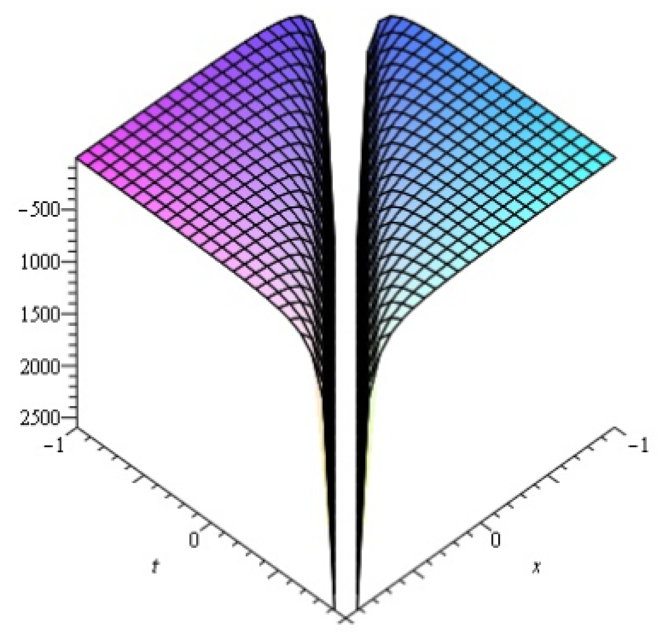
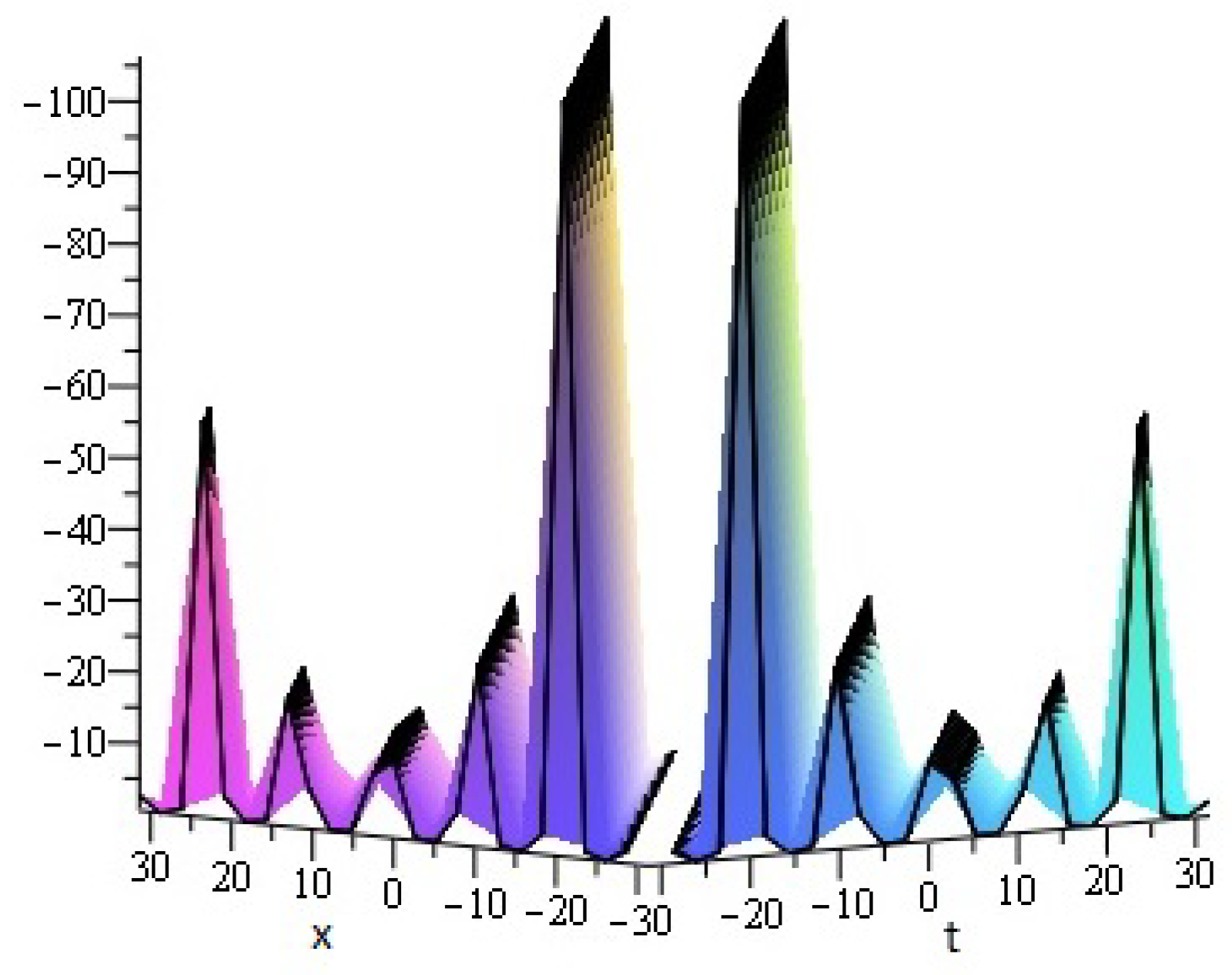
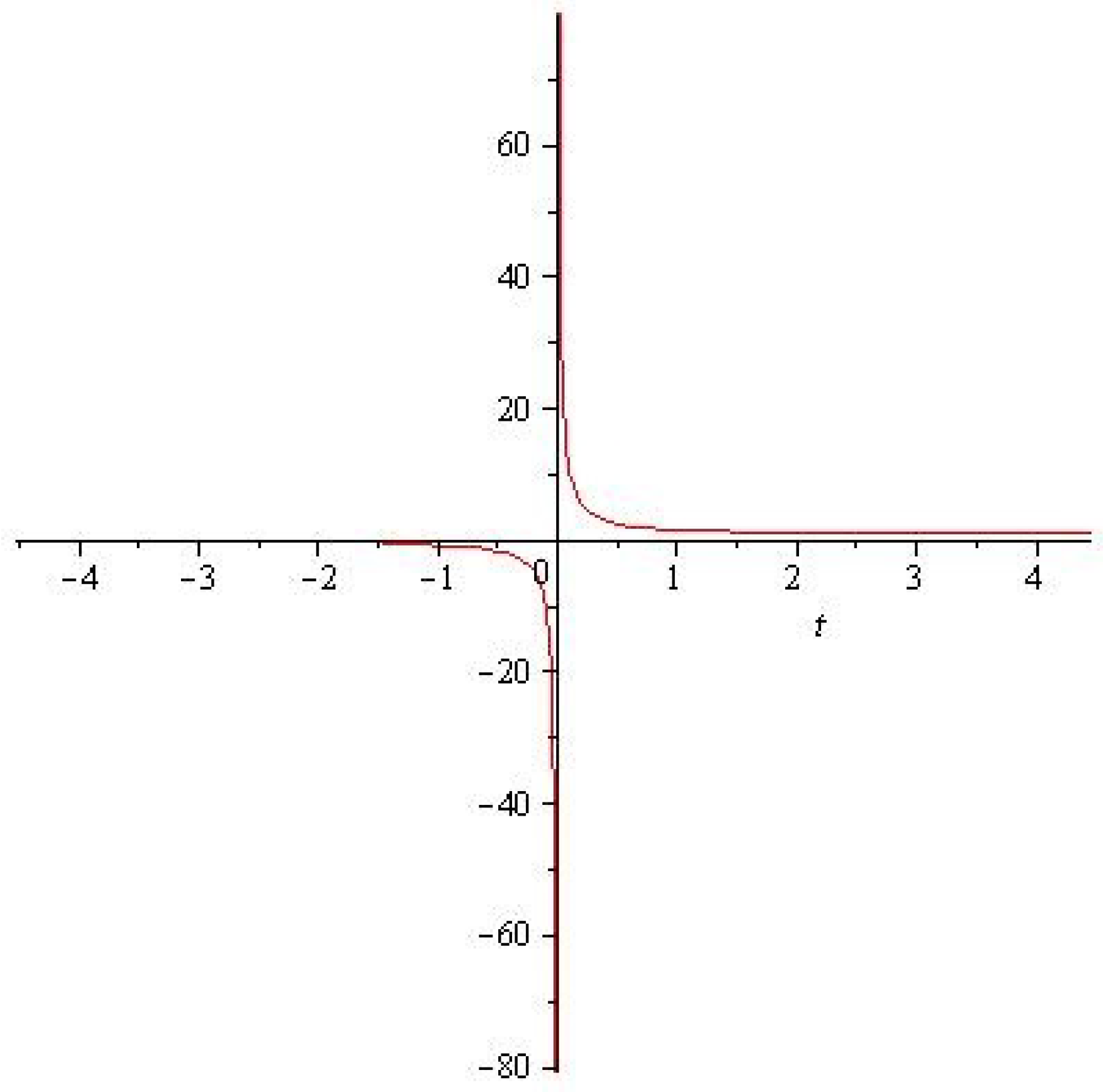
5. Description of Figures

Figure 1 represents a hyperbolic solitary wave solution for problem 1 graphically, corresponding to $\alpha =c=k=e=1$, $A=a=2$, $b=-1$ and $B=\frac{11}{12}$.

Figure 2 represents the graph of $V_4(x,t)$ which is a exact periodic travelling wave solution for the fixed values $\alpha =c=k=e=A=b=1$, $a=2$ and $B=\frac{1}{3}$ in problem 1. A periodic solution is a travelling wave solution that is periodic.

Figure 3 represents the graph of Equation (24) which is a exact hyperbolic travelling wave solution for the fixed values $\alpha =1$, $A=-1$, $c=0$ and $k=\frac{1}{2}$ in problem 2. The value $c=0$ vanishes x from the solution therefore, this figure shows a graph of hyperbola in two dimensions.

6. Conclusions

In this research article, the $(G^{{}^{\prime }}/G)$-expansion method is applied for the analytical solutions of fractional Klein-Gordon and Gas Dynamics equations. The fractional derivative is described in Jumarie’s sense. The complex transformation is used to reduced the given FPDEs into ODEs. The $(G^{{}^{\prime }}/G)$-expansion method is implemented in series form with some unknown coefficients, which provide the system of algebraic equations containing these unknowns. The system of equations is solved by Maple software to determine these unknown. Thus the $(G^{{}^{\prime }}/G)$ solution is obtained for the given problems in hyperbolic, trigonometric and rational families. The proposed method is an efficient analytical technique as compared to other analytical methods because it provides several periodic and solitary travelling wave solutions with some parameters. The results obtained by the proposed method play a vital role in exposing the inner mechanism of physical phenomena and provide distinct solutions of different physical structures in non-linear science. Besides physical applications, the series forms solutions of method help the numerical solvers to compare the accuracy of their results and assist them in stability analysis.

The procedure of $(G^{{}^{\prime }}/G)$-expansion method is easy and accurate for solving the given problems. Therefore, the proposed method can be extended to other FPDEs.

References

1. Almeida, R.; Bastos, N.R.O.; Teresa, M.; Monteiro, T. Modeling some real phenomena by fractional differential equationsh. Math. Methods Appl. Sci. 2016, 39, 4846–4855. [Google Scholar] [CrossRef]
2. Sun, H.; Zhang, Y.; Baleanu, D.; Chen, W.; Chen, Y. A new collection of real world applications of fractional calculus in science and engineering. Commun. Nonlinear Sci. Numer. Simul. 2018, 64, 213–231. [Google Scholar] [CrossRef]
3. Tarasov, V. Generalized memory: Fractional calculus approach. Fractal Fract. 2018, 2, 23. [Google Scholar] [CrossRef]
4. El-Misiery, A.E.M.; Ahmed, E. On a fractional model for earthquakes. Appl. Math. Comput. 2006, 178, 207–211. [Google Scholar] [CrossRef]
5. Wu, J. A wavelet operational method for solving fractional partial differential equations numerically. Appl. Math. Comput. 2009, 214, 31–40. [Google Scholar] [CrossRef]
6. Zhang, W.; Li, J.; Yang, Y. A fractional diffusion-wave equation with non-local regularization for image denoising. Signal Process. 2014, 103, 6–15. [Google Scholar] [CrossRef]
7. Hu, Y.; Øksendal, B. Fractional white noise calculus and applications to finance. Infin. Dimens. Anal. Quantum Probab. Relat. Top. 2003, 6, 1–32. [Google Scholar] [CrossRef]
8. Nagy, A.M. Numerical solution of time fractional nonlinear Klein-Gordon equation using Sinc-Chebyshev collocation method. Appl. Math. Comput. 2017, 310, 139–148. [Google Scholar] [CrossRef]
9. Garrappa, R. Numerical solution of fractional differential equations: A survey and a software tutorial. Mathematics 2018, 6, 16. [Google Scholar] [CrossRef]
10. Jiang, J.; Feng, Y.; Li, S. Exact Solutions to the Fractional Differential Equations with Mixed Partial Derivatives. Axioms 2018, 7, 10. [Google Scholar] [CrossRef]
11. Song, J.; Yin, F.; Cao, X.; Lu, F. Fractional variational iteration method versus Adomian’s decomposition method in some fractional partial differential equations. J. Appl. Math. 2013, 2013, 392567. [Google Scholar] [CrossRef]
12. Duan, J.; Rach, R.; Baleanu, D.; Wazwaz, A. A review of the Adomian decomposition method and its applications to fractional differential equations. Commun. Fract. Calc. 2012, 3, 73–99. [Google Scholar]
13. Mahmood, S.; Shah, R.; Arif, M. Laplace Adomian Decomposition Method for Multi Dimensional Time Fractional Model of Navier-Stokes Equation. Symmetry 2019, 11, 149. [Google Scholar] [CrossRef]
14. Wang, Q. Homotopy perturbation method for fractional KdV-Burgers equation. Chaos Solitons Fractals 2008, 35, 843–850. [Google Scholar] [CrossRef]
15. Raslan, K.R.; Ali, K.K.; Shallal, M.A. The modified extended tanh method with the Riccati equation for solving the space-time fractional EW and MEW equations. Chaos Solitons Fractals 2017, 103, 404–409. [Google Scholar] [CrossRef]
16. Alzaidy, J.F. Fractional sub-equation method and its applications to the space-time fractional differential equations in mathematical physics. Br. J. Math. Comput. Sci. 2013, 3, 153. [Google Scholar] [CrossRef]
17. Tasbozan, O.; Çenesiz, Y.; Kurt, A. New solutions for conformable fractional Boussinesq and combined KdV-mKdV equations using Jacobi elliptic function expansion method. Eur. Phys. J. Plus 2016, 131, 244. [Google Scholar] [CrossRef]
18. Meerschaert, M.M.; Tadjeran, C. Finite difference approximations for fractional advection–dispersion flow equations. J. Comput. Appl. Math. 2004, 172, 65–77. [Google Scholar] [CrossRef] [Green Version]
19. Jiang, Y.; Ma, J. High-order finite element methods for time-fractional partial differential equations. J. Comput. Appl. Math. 2011, 235, 3285–3290. [Google Scholar] [CrossRef] [Green Version]
20. Zheng, B. Exp-function method for solving fractional partial differential equations. Sci. World J. 2013, 2013, 465723. [Google Scholar] [CrossRef]
21. Shang, N.; Zheng, B. Exact solutions for three fractional partial differential equations by the ( G G )-expansion method. Int. J. Appl. Math. 2013, 43, 114–119. [Google Scholar]
22. Zhang, Y. Solving STO and KD equations with modified Riemann–Liouville derivative using improved ( G G )-expansion function method. Int. J. Appl. Math. 2015, 45, 16–22. [Google Scholar]
23. Shakeel, M.; Mohyud-Din, S.T. New ( G G )-expansion method and its application to the zakharov-kuznetsov-benjamin-bona-mahony (ZK–BBM) equation. J. Assoc. Arab Univ. Basic Appl. Sci. 2015, 18, 66–81. [Google Scholar] [CrossRef]
24. Zheng, B. ( G G )-expansion method for solving fractional partial differential equations in the theory of mathematical physics. Commun. Theor. Phys. 2012, 58, 623. [Google Scholar] [CrossRef]
25. Zayed, E.M.E.; Amer, Y.A.; Shohib, R.M.A. Exact traveling wave solutions for nonlinear fractional partial differential equations using the improved ( G G )-expansion method. Int. J. Eng. 2014, 4, 8269. [Google Scholar]
26. Abuteen, E.; Freihat, A.; Al-Smadi, M.; Khalil, H.; Khan, R.A. Approximate series solution of nonlinear, fractional Klein-Gordon equations using fractional reduced differential transform method. arXiv 2017, arXiv:1704.06982. [Google Scholar] [CrossRef]
27. Acan, O.; Baleanu, D. A new numerical technique for solving fractional partial differential equations. arXiv 2017, arXiv:1704.02575. [Google Scholar] [CrossRef]
28. Chowdhury, M.S.H.; Hashim, I. Application of homotopy-perturbation method to Klein–Gordon and sine-Gordon equations. Chaos Solitons Fractals 2009, 39, 1928–1935. [Google Scholar] [CrossRef]
29. Kheiri, H.; Shahi, S.; Mojaver, A. Analytical solutions for the fractional Klein-Gordon equation. Comput. Methods Differ. Equ. 2014, 2, 99–114. [Google Scholar]
30. Singh, J.; Kumar, D.; Kılıçman, A. Homotopy perturbation method for fractional gas dynamics equation using Sumudu transform. Abst. Appl. Anal. 2013, 2013, 934060. [Google Scholar] [CrossRef]
31. Tamsir, M.; Srivastava, V.K. Revisiting the approximate analytical solution of fractional-order gas dynamics equation. Alex. Eng. J. 2016, 55, 867–874. [Google Scholar] [CrossRef]
32. Alam, M.; Rahman, M.; Islam, R.; Roshid, H. Application of the new extended (G’/G)-expansion method to find exact solutions for nonlinear partial differential equation. Comput. Methods Differ. Equ. 2015, 3, 59–69. [Google Scholar]
33. Ozis, T.; Aslan, I. Symbolic computation and construction of new exact traveling wave solutions to Fitzhugh-Nagumo and Klein-Gordon equations. Z. Naturforschung A 2009, 64, 15. [Google Scholar]
Figure 1. For problem 1, the graph of V 2 ( x , t ) for the values α = c = k = e = 1 , A = a = 2 , b = 1 and B = 11 12 shows the hyperbolic solitary wave solution.
Symmetry 11 00566 g001
Figure 2. For problem 1, the graph of V 4 ( x , t ) for the values α = c = k = e = A = b = 1 , a = 2 and B = 1 3 shows the periodic solitary wave solution.
Symmetry 11 00566 g002
Figure 3. For problem 2, the graph of V 4 ( x , t ) for the values α = 1 , A = 1 , c = 0 and k = 1 2 shows the hyperbolic solitary wave solution.
Symmetry 11 00566 g003