System Identification Based on Tensor Decompositions: A Trilinear Approach

Abstract

The theory of nonlinear systems can currently be encountered in many important fields, while the nonlinear behavior of electronic systems and devices has been studied for a long time. However, a global approach for dealing with nonlinear systems does not exist and the methods to address this problem differ depending on the application and on the types of nonlinearities. An interesting category of nonlinear systems is one that can be regarded as an ensemble of (approximately) linear systems. Some popular examples in this context are nonlinear electronic devices (such as acoustic echo cancellers, which are used in applications for two-party or multi-party voice communications, e.g., videoconferencing), which can be modeled as a cascade of linear and nonlinear systems, similar to the Hammerstein model. Multiple-input/single-output (MISO) systems can also be regarded as separable multilinear systems and be treated using the appropriate methods. The high dimension of the parameter space in such problems can be addressed with methods based on tensor decompositions and modelling. In recent work, we focused on a particular type of multilinear structure—namely the bilinear form (i.e., two-dimensional decompositions)—in the framework of identifying spatiotemporal models. In this paper, we extend the work to the decomposition of more complex systems and we propose an iterative Wiener filter tailored for the identification of trilinear forms (where third-order tensors are involved), which can then be further extended to higher order multilinear structures. In addition, we derive the least-mean-square (LMS) and normalized LMS (NLMS) algorithms tailored for such trilinear forms. Simulations performed in the context of system identification (based on the MISO system approach) indicate the good performance of the proposed solution, as compared to conventional approaches.

1. Introduction

The approximation of nonlinear systems can be performed using a finite sum of the Volterra series expansion that relates the system’s inputs and outputs. This method has been studied since the 1960s [1,2,3] and used in different applications, for example, Reference [4,5,6], among others. In this context, bilinear forms have been used to approximate a large class of nonlinear systems, where the bilinear component is interpreted in terms of an input-output relation (meaning that it is defined with respect to the data). Consequently, the bilinear system may be regarded as one of the simplest recursive nonlinear systems.

More recently, a new approach was introduced in Reference [7], where the bilinear term is considered within the framework of a multiple-input/single-output (MISO) system, and it is defined with respect to the spatiotemporal model’s impulse responses. A particular case of this type of system is the Hammerstein model [8]; in this scenario, a single-input signal passes through a nonlinear block and a linear system, which are cascaded. Recently, adaptive solutions were proposed for the study of such bilinear forms in the context of system identification [9,10,11]. The bilinear approach is suitable for a particular form of the decomposition, which involves only two terms (i.e., two systems). In some cases, it would be useful to exploit a higher-order decomposition, which could improve the overall performance in terms of both complexity and efficiency.

Motivated by the good performance of these approaches in the study of bilinear forms, we aim to further extend this approach to higher-order multilinear in parameters’ systems. Applications, such as multichannel equalization [12], nonlinear acoustic devices for echo cancellation [13], multiple-input/multiple-output (MIMO) communication systems [14,15] and others, can be addressed within the framework of multilinear systems. Because many of these applications can be formulated in terms of system identification problems [16], it is of interest to estimate a model based on the available and observed data, which are usually the input and the output of the system. The challenges that usually occur in such system identification tasks may be represented by a high length of the finite impulse response filter [17,18], which may employ hundreds or even thousands of coefficients. Moreover, another possible issue is the large parameter space [19,20]. Nowadays, such scenarios are related to very important topics, for example, big data [21], machine learning [22], and source separation [23]. Usually, they are addressed based on tensor decompositions and modelling [24,25,26,27]. These techniques mainly exploit the Kronecker product decomposition [28], which further allows the reformulation of a high-dimension problem as low-dimension models, which can be tensorized together.

In this paper, we propose an iterative Wiener filter tailored for third-order systems (i.e., trilinear forms), together with adaptive solutions for such problems—namely the least-mean-square (LMS) and normalized LMS (NLMS) algorithms. Following this development, the solution can then be extended to higher-order multilinear systems. The proposed approach presents an advantage from the perspective of exploiting the decomposition of the global impulse response. One potential limitation of such a method is related to the particular form of the global impulse response to be identified, which is a result of separable systems. In perspective, it would be useful to extend this approach to identify more general forms of impulse responses. Recently, we developed such ideas in References [29,30], based on the Wiener filter and the recursive least-squares (RLS) algorithm, by exploiting the nearest Kronecker product decomposition and the related low-rank approximation.

The rest of this paper is organized as follows: In Section 2, a brief theory of tensors is provided, which is necessary for the following developments; next, in Section 3, the iterative Wiener filter tailored for the identification of trilinear forms is proposed; Section 4 contains the derivation of the trilinear forms for the LMS and NLMS adaptive algorithms; simulation results are provided in Section 5, while Section 6 concludes the paper.

2. Background on Tensors

A tensor is a multidimensional array of data the entries of which are referred by using multiple indices [31,32]. A tensor, a matrix, a vector, and a scalar can be denoted by $\mathcal{A}$, $\mathbf{A}$, $\mathbf{a}$, and a, respectively. In this paper, we are only interested in the third-order tensor $\mathcal{A}\in {\mathbb{R}}^{L_1\times L_2\times L_3}$, meaning that its elements are real-valued and its dimension is $L_1\times L_2\times L_3$. For a third-order tensor, the first and second indices $l_1$ and $l_2$ correspond to the row and column, respectively—as in a matrix—while the third index $l_3$ corresponds to the tube and describes its depth. These three indices describe the three different modes. The entries of the different order tensors are denoted by ${\left(\mathcal{A}\right)}_{l_1{l}_2{l}_3}=a_{l_1{l}_2{l}_3}$, ${\left(\mathbf{A}\right)}_{l_1{l}_2}=a_{l_1{l}_2}$, and ${\left(\mathbf{a}\right)}_{l_1}=a_{l_1}$, for $l_1=1,2,\dots ,L_1$, $l_2=1,2,\dots ,L_2$, and $l_3=1,2,\dots ,L_3$.

The notion of vectorization, consisting of transforming a matrix into a vector, is very well known. Matricization does somewhat the same thing but from a third-order tensor into a large matrix. Depending on which index’s elements are considered first, we have matricization along three different modes [24,25]:

$$\begin{array}{cc}{\mathbf{A}}_{\left[1\right]}\hfill & ={\mathbf{A}}_{:,1:L_2,1:L_3}\hfill \\ & =\left[\begin{array}{ccc}{\mathbf{A}}_{::1}& \cdots & {\mathbf{A}}_{::L_3}\end{array}\right],{\mathbf{A}}_{\left[1\right]}\in {\mathbb{R}}^{L_1\times L_2{L}_3},\hfill \\ {\mathbf{A}}_{\left[2\right]}\hfill & ={\mathbf{A}}_{1:L_1,:,1:L_3},{\mathbf{A}}_{\left[2\right]}\in {\mathbb{R}}^{L_2\times L_1{L}_3},\hfill \\ {\mathbf{A}}_{\left[3\right]}\hfill & ={\mathbf{A}}_{1:L_1,1:L_2,:},{\mathbf{A}}_{\left[3\right]}\in {\mathbb{R}}^{L_3\times L_1{L}_2},\hfill \end{array}$$

where ${\mathbf{A}}_{::l_3}\in {\mathbb{R}}^{L_1\times L_2},l_3=1,2,\dots ,L_3$ are the frontal slices. Hence, the vectorization of a tensor is

$$\begin{array}{cc}\mathrm{vec}\left(\mathcal{A}\right)\hfill & =\mathrm{vec}\left({\mathbf{A}}_{\left[1\right]}\right)=\left[\begin{array}{c}\mathrm{vec}\left({\mathbf{A}}_{::1}\right)\\ ⋮\\ \mathrm{vec}\left({\mathbf{A}}_{::L_3}\right)\end{array}\right]\in {\mathbb{R}}^{L_1{L}_2{L}_3}.\hfill \end{array}$$

Let ${\mathbf{b}}_1$, ${\mathbf{b}}_2$, and ${\mathbf{b}}_3$ be vectors of length $L_1$, $L_2$, and $L_3$, respectively, whose elements are $b_{1l_1}$, $b_{2l_2}$, and $b_{3l_3}$. A rank-1 tensor (of dimension $L_1\times L_2\times L_3$) is defined as

$$\begin{array}{cc}\mathcal{B}\hfill & ={\mathbf{b}}_1\circ {\mathbf{b}}_2\circ {\mathbf{b}}_3,\hfill \end{array}$$

(1)

where ∘ is the vector outer product and the elements of $\mathcal{B}$ are given by ${\left(\mathcal{B}\right)}_{l_1{l}_2{l}_3}=b_{1l_1}{b}_{2l_2}{b}_{3l_3}$. The frontal slices of $\mathcal{B}$ in Equation (1) are ${\mathbf{B}}_{::l_3}={\mathbf{b}}_1{\mathbf{b}}_2^T{b}_{3l_3}\in {\mathbb{R}}^{L_1\times L_2},l_3=1,2,\dots ,L_3$. In particular, we have $\mathbf{B}={\mathbf{b}}_1\circ {\mathbf{b}}_2={\mathbf{b}}_1{\mathbf{b}}_2^T$, where ${}^T$ is the transpose operator. Therefore, the rank of a tensor $\mathcal{A}$, denoted $\mathrm{rank}\left(\mathcal{A}\right)$, is defined as the minimum number of rank-1 tensors that generate $\mathcal{A}$ as their sum.

The inner product between two tensors $\mathcal{A}$ and $\mathcal{B}$ of the same dimension is

$$\begin{array}{c}\langle \mathcal{A},\mathcal{B}\rangle =\sum _{l_1=1}^{L_1}\sum _{l_2=1}^{L_2}\sum _{l_3=1}^{L_3}{a}_{l_1{l}_2{l}_3}{b}_{l_1{l}_2{l}_3}={\mathrm{vec}}^T\left(\mathcal{B}\right)\mathrm{vec}\left(\mathcal{A}\right).\hfill \end{array}$$

It is important to be able to multiply a tensor with a matrix [26,27]. Let the tensor be $\mathcal{A}\in {\mathbb{R}}^{L_1\times L_2\times L_3}$ and the matrix be ${\mathbf{M}}_1\in {\mathbb{R}}^{M_1\times L_1}$. The mode-1 product between the tensor $\mathcal{A}$ and the matrix ${\mathbf{M}}_1$ gives the tensor:

$$\begin{array}{cc}\mathcal{U}\hfill & =\mathcal{A}{\times }_1{\mathbf{M}}_1,\mathcal{U}\in {\mathbb{R}}^{M_1\times L_2\times L_3},\hfill \end{array}$$

(2)

whose entries are $u_{m_1{l}_2{l}_3}={\sum }_{l_1=1}^{L_1}{a}_{l_1{l}_2{l}_3}{m}_{m_1{l}_1}$, for $m_1=1,2,\dots ,M_1$, and ${\mathbf{U}}_{\left[1\right]}={\mathbf{M}}_1{\mathbf{A}}_{\left[1\right]}$. In the same way, with the matrix ${\mathbf{M}}_2\in {\mathbb{R}}^{M_2\times L_2}$, the mode-2 product between the tensor $\mathcal{A}$ and the matrix ${\mathbf{M}}_2$ gives the tensor:

$$\begin{array}{cc}\mathcal{U}\hfill & =\mathcal{A}{\times }_2{\mathbf{M}}_2,\mathcal{U}\in {\mathbb{R}}^{L_1\times M_2\times L_3},\hfill \end{array}$$

(3)

whose entries are $u_{l_1{m}_2{l}_3}={\sum }_{l_2=1}^{L_2}{a}_{l_1{l}_2{l}_3}{m}_{m_2{l}_2}$, for $m_2=1,2,\dots ,M_2$, and ${\mathbf{U}}_{\left[2\right]}={\mathbf{M}}_2{\mathbf{A}}_{\left[2\right]}$. Finally, with the matrix ${\mathbf{M}}_3\in {\mathbb{R}}^{M_3\times L_3}$, the mode-3 product between the tensor $\mathcal{A}$ and the matrix ${\mathbf{M}}_3$ gives the tensor:

$$\begin{array}{cc}\mathcal{U}\hfill & =\mathcal{A}{\times }_3{\mathbf{M}}_3,\mathcal{U}\in {\mathbb{R}}^{L_1\times L_2\times M_3},\hfill \end{array}$$

(4)

whose entries are $u_{l_1{l}_2{m}_3}={\sum }_{l_3=1}^{L_3}{a}_{l_1{l}_2{l}_3}{m}_{m_3{l}_3}$, for $m_3=1,2,\dots ,M_3$, and ${\mathbf{U}}_{\left[3\right]}={\mathbf{M}}_3{\mathbf{A}}_{\left[3\right]}$.

The multiplication of $\mathcal{A}$ with the row vectors ${\mathbf{b}}_1^T$, ${\mathbf{b}}_2^T$, and ${\mathbf{b}}_3^T$ (see the components of $\mathcal{B}$ in Equation (1)) gives the scalar:

$$\begin{array}{cc}c\hfill & =\mathcal{A}{\times }_1{\mathbf{b}}_1^T{\times }_2{\mathbf{b}}_2^T{\times }_3{\mathbf{b}}_3^T=\sum _{l_1=1}^{L_1}\sum _{l_2=1}^{L_2}\sum _{l_3=1}^{L_3}{a}_{l_1{l}_2{l}_3}{b}_{1l_1}{b}_{2l_2}{b}_{3l_3}.\hfill \end{array}$$

(5)

In particular, we have

$$\begin{array}{cc}c\hfill & =\mathbf{A}{\times }_1{\mathbf{b}}_1^T{\times }_2{\mathbf{b}}_2^T=\sum _{l_1=1}^{L_1}\sum _{l_2=1}^{L_2}{a}_{l_1{l}_2}{b}_{1l_1}{b}_{2l_2}={\mathbf{b}}_1^T\mathbf{A}{\mathbf{b}}_2\hfill \end{array}$$

(6)

and

$$\begin{array}{cc}c\hfill & =\mathbf{a}{\times }_1{\mathbf{b}}_1^T=\sum _{l_1=1}^{L_1}{a}_{l_1}{b}_{1l_1}={\mathbf{b}}_1^T\mathbf{a}.\hfill \end{array}$$

(7)

It is easy to check that Equations (5)–(7) are trilinear (with respect to ${\mathbf{b}}_1$, ${\mathbf{b}}_2$, and ${\mathbf{b}}_3$), bilinear (with respect to ${\mathbf{b}}_1$ and ${\mathbf{b}}_2$), and linear (with respect to ${\mathbf{b}}_1$) forms, respectively.

We can express Equation (6) as

$$\begin{array}{cc}c\hfill & =\mathrm{tr}\left({\mathbf{b}}_2{\mathbf{b}}_1^T\mathbf{A}\right)=\mathrm{tr}\left[{\left({\mathbf{b}}_1{\mathbf{b}}_2^T\right)}^T\mathbf{A}\right]={\mathrm{vec}}^T\left({\mathbf{b}}_1{\mathbf{b}}_2^T\right)\mathrm{vec}\left(\mathbf{A}\right)\hfill \\ & ={\left({\mathbf{b}}_2\otimes {\mathbf{b}}_1\right)}^T\mathrm{vec}\left(\mathbf{A}\right),\hfill \end{array}$$

(8)

where $\mathrm{tr}(·)$ represents the trace of a square matrix and ⊗ denotes the Kronecker product. Expression (5) can also be written in a more convenient way. Indeed, we have

$$\begin{array}{cc}c\hfill & =\langle \mathcal{A},\mathcal{B}\rangle ={\mathrm{vec}}^T\left(\mathcal{B}\right)\mathrm{vec}\left(\mathcal{A}\right)\hfill \\ & ={\mathrm{vec}}^T\left({\mathbf{b}}_1\circ {\mathbf{b}}_2\circ {\mathbf{b}}_3\right)\mathrm{vec}\left(\mathcal{A}\right)\hfill \\ & ={\left({\mathbf{b}}_3\otimes {\mathbf{b}}_2\otimes {\mathbf{b}}_1\right)}^T\mathrm{vec}\left(\mathcal{A}\right),\hfill \end{array}$$

(9)

where $\mathcal{B}$ is defined in Equation (1).

3. Trilinear Wiener Filter

Let us consider the following signal model, which is used in system identification tasks:

$$\begin{array}{cc}d\left(t\right)\hfill & =y\left(t\right)+v\left(t\right)\hfill \\ & =\mathcal{X}\left(t\right){\times }_1{\mathbf{h}}_1^T{\times }_2{\mathbf{h}}_2^T{\times }_3{\mathbf{h}}_3^T+v\left(t\right)\hfill \\ & =\sum _{l_1=1}^{L_1}\sum _{l_2=1}^{L_2}\sum _{l_3=1}^{L_3}{x}_{l_1{l}_2{l}_3}\left(t\right)h_{1l_1}{h}_{2l_2}{h}_{3l_3}+v\left(t\right),\hfill \end{array}$$

(10)

where $d\left(t\right)$ is the desired (also known as reference) signal at time index t, $y\left(t\right)$ is the output signal of a MISO system and $v\left(t\right)$ is a zero-mean additive noise, uncorrelated with the input signals. The zero-mean input signals can be described in a tensorial form $\mathcal{X}\left(t\right)\in {\mathbb{R}}^{L_1\times L_2\times L_3}$:

$$\begin{array}{cc}{\left(\mathcal{X}\right)}_{l_1{l}_2{l}_3}\left(t\right)\hfill & =x_{l_1{l}_2{l}_3}\left(t\right),l_k=1,2,\dots ,L_k,k=1,2,3,\hfill \end{array}$$

and the three impulse responses ${\mathbf{h}}_k,k=1,2,3$, of lengths $L_1$, $L_2$, and $L_3$, respectively, can be written as

$$\begin{array}{c}{\mathbf{h}}_k={\left[\begin{array}{cccc}{h}_{k1}& h_{k2}& \cdots & h_{k{L}_k}\end{array}\right]}^T,k=1,2,3.\hfill \end{array}$$

It can be seen that $y\left(t\right)$ represents a trilinear form because it is a linear function of each of the vectors ${\mathbf{h}}_k,k=1,2,3$, if the other two are kept fixed. The trilinear form can be regarded as an extension of the bilinear form [7].

Starting from the three impulse responses of the MISO system, a rank-1 tensor of dimension $L_1\times L_2\times L_3$ can be constructed in the following way:

$$\begin{array}{cc}\mathcal{H}\hfill & ={\mathbf{h}}_1\circ {\mathbf{h}}_2\circ {\mathbf{h}}_3,\hfill \end{array}$$

(11)

where

$$\begin{array}{cc}{\left(\mathcal{H}\right)}_{l_1{l}_2{l}_3}\hfill & =h_{1l_1}{h}_{2l_2}{h}_{3l_3},l_k=1,2,\dots ,L_k,k=1,2,3.\hfill \end{array}$$

Consequently, the output signal becomes

$$\begin{array}{c}y\left(t\right)={\mathrm{vec}}^T\left(\mathcal{H}\right)\mathrm{vec}\left[\mathcal{X}\left(t\right)\right],\hfill \end{array}$$

(12)

where

$$\begin{array}{cc}\mathrm{vec}\left(\mathcal{H}\right)\hfill & =\left[\begin{array}{c}\mathrm{vec}\left({\mathbf{H}}_{::1}\right)\\ ⋮\\ \mathrm{vec}\left({\mathbf{H}}_{::L_3}\right)\end{array}\right]={\mathbf{h}}_3\otimes {\mathbf{h}}_2\otimes {\mathbf{h}}_1\triangleq \mathbf{h},\hfill \end{array}$$

(13)

$$\begin{array}{cc}\mathrm{vec}\left[\mathcal{X}\left(t\right)\right]\hfill & =\left[\begin{array}{c}\mathrm{vec}\left[{\mathbf{X}}_{::1}\left(t\right)\right]\\ ⋮\\ \mathrm{vec}\left[{\mathbf{X}}_{::L_3}\left(t\right)\right]\end{array}\right]\triangleq \mathbf{x}\left(t\right),\hfill \end{array}$$

(14)

${\mathbf{H}}_{::l_3}$ and ${\mathbf{X}}_{::l_3}\left(t\right)$ (with $l_3=1,2,\dots ,L_3$) are the frontal slices of $\mathcal{H}$ and $\mathcal{X}\left(t\right)$, respectively, while $\mathbf{h}$ and $\mathbf{x}\left(t\right)$ denote two long vectors, each of them having $L_1{L}_2{L}_3$ elements. Hence, the output signal can be expressed as

$$\begin{array}{c}y\left(t\right)={\mathbf{h}}^T\mathbf{x}\left(t\right).\hfill \end{array}$$

(15)

In this framework, the aim is to estimate the global impulse response $\mathbf{h}$. For that, first we define the error signal:

$$\begin{array}{c}e\left(t\right)=d\left(t\right)-\widehat{y}\left(t\right)=d\left(t\right)-{\widehat{\mathbf{h}}}^T\mathbf{x}\left(t\right),\hfill \end{array}$$

(16)

where $\widehat{y}\left(t\right)={\widehat{\mathbf{h}}}^T\mathbf{x}\left(t\right)$ represents the estimated signal, obtained using the impulse response $\widehat{\mathbf{h}}$ of length $L_1{L}_2{L}_3$.

Based on Equation (16), let us consider the mean-squared error (MSE) optimization criterion, that is, the minimization of the cost function:

$$\begin{array}{c}J\left(\widehat{\mathbf{h}}\right)=E\left[e^2\left(t\right)\right],\hfill \end{array}$$

(17)

where $E[·]$ denotes mathematical expectation. Using Equation (16) in Equation (17), together with the notation ${\sigma }_d^2=E\left[d^2\left(t\right)\right]$ (the variance of the reference signal), $\mathbf{p}=E\left[\mathbf{x}\left(t\right)d\left(t\right)\right]$ (the cross-correlation vector between the input and the reference signals) and $\mathbf{R}=E\left[\mathbf{x}\left(t\right){\mathbf{x}}^T\left(t\right)\right]$ (the covariance matrix of the input signal), the cost function can be developed as

$$\begin{array}{c}J\left(\widehat{\mathbf{h}}\right)={\sigma }_d^2-2{\widehat{\mathbf{h}}}^T\mathbf{p}+{\widehat{\mathbf{h}}}^T\mathbf{R}\widehat{\mathbf{h}}.\hfill \end{array}$$

(18)

By minimizing Equation (18), we obtain the well-known Wiener filter:

$$\begin{array}{c}{\widehat{\mathbf{h}}}_{\mathrm{W}}={\mathbf{R}}^{-1}\mathbf{p}.\hfill \end{array}$$

(19)

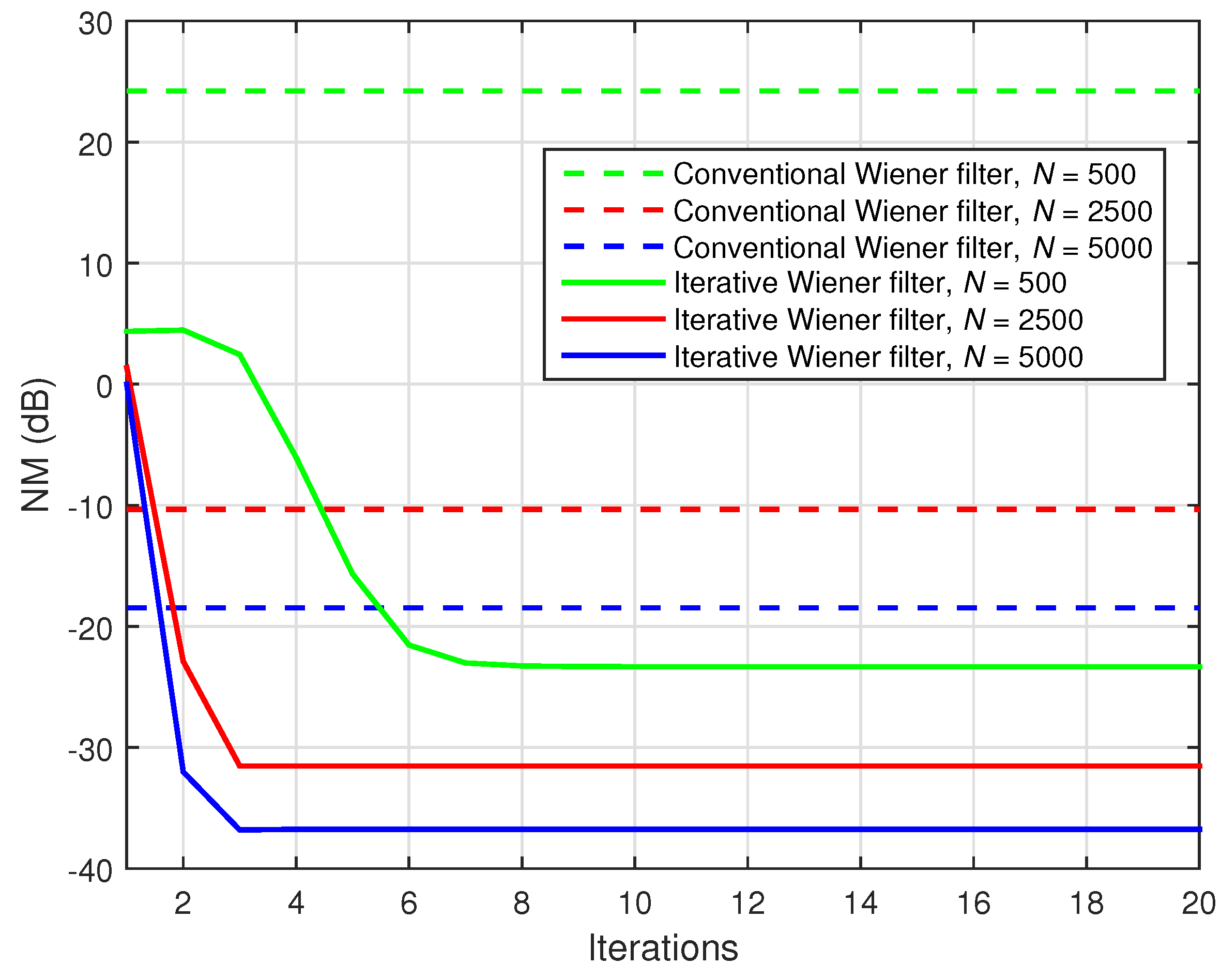
As we can see, the dimension of the covariance matrix is $L_1{L}_2{L}_3\times L_1{L}_2{L}_3$, thus requiring a large amount of data (much more than $L_1{L}_2{L}_3$ samples) to obtain a good estimate of it. Furthermore, $\mathbf{R}$ could be very ill-conditioned because of its huge size. As a result, the solution ${\widehat{\mathbf{h}}}_{\mathrm{W}}$ will be very inaccurate, to say the least, in practice.

On the other hand, as we notice from Equation (13), the global impulse response $\mathbf{h}$ (with $L_1{L}_2{L}_3$ coefficients) results based on a combination of the shorter impulse responses ${\mathbf{h}}_k,k=1,2,3$, with $L_1$, $L_2$, and $L_3$ coefficients, respectively. In fact, we only need $L_1+L_2+L_3$ different elements to form $\mathbf{h}$, even though this global impulse response is of length $L_1{L}_2{L}_3$. This represents the motivation behind an alternative approach to the conventional Wiener solution. Similar to Equation (13), the estimate of the global system can be decomposed as

$$\begin{array}{c}\widehat{\mathbf{h}}={\widehat{\mathbf{h}}}_3\otimes {\widehat{\mathbf{h}}}_2\otimes {\widehat{\mathbf{h}}}_1,\hfill \end{array}$$

(20)

where ${\widehat{\mathbf{h}}}_k,k=1,2,3$ are three impulse responses of lengths $L_1$, $L_2$, and $L_3$, respectively, which represent the estimates of the individual impulse responses ${\mathbf{h}}_k,k=1,2,3$. Nevertheless, we should note that there is no unique solution related to the decomposition in Equation (20), since for any constants ${\alpha }_1,{\alpha }_2$, and ${\alpha }_3$, with ${\alpha }_1{\alpha }_2{\alpha }_3=1$, we have $\widehat{\mathbf{h}}={\widehat{\mathbf{h}}}_3\otimes {\widehat{\mathbf{h}}}_2\otimes {\widehat{\mathbf{h}}}_1={\alpha }_3{\widehat{\mathbf{h}}}_3\otimes {\alpha }_2{\widehat{\mathbf{h}}}_2\otimes {\alpha }_1{\widehat{\mathbf{h}}}_1$. Consequently, ${\alpha }_k{\widehat{\mathbf{h}}}_k,k=1,2,3$ also represents a set of solutions for our problem. Nevertheless, the global system impulse response—$\mathbf{h}$—can be identified with no scaling ambiguity.

Next, we propose an iterative alternative to the conventional Wiener filter, following the decomposition from Equation (20). First, we can easily verify that

$$\begin{array}{}\mathrm{(21)}& \widehat{\mathbf{h}}\hfill & =\left({\widehat{\mathbf{h}}}_3\otimes {\widehat{\mathbf{h}}}_2\otimes {\mathbf{I}}_{L_1}\right){\widehat{\mathbf{h}}}_1\hfill \mathrm{(22)}& \hfill & =\left({\widehat{\mathbf{h}}}_3\otimes {\mathbf{I}}_{L_2}\otimes {\widehat{\mathbf{h}}}_1\right){\widehat{\mathbf{h}}}_2\hfill \mathrm{(23)}& \hfill & =\left({\mathbf{I}}_{L_3}\otimes {\widehat{\mathbf{h}}}_2\otimes {\widehat{\mathbf{h}}}_1\right){\widehat{\mathbf{h}}}_3,\hfill \end{array}$$

where ${\mathbf{I}}_{L_k}$ is the identity matrix of size $L_k\times L_k$, for $k=1,2,3$. Based on the previous relations, the cost function from Equation (18) can be expressed in three different ways. For example, using Equation (21), we obtain

$$\begin{array}{cc}J\left({\widehat{\mathbf{h}}}_1,{\widehat{\mathbf{h}}}_2,{\widehat{\mathbf{h}}}_3\right)\hfill & ={\sigma }_d^2-2{\widehat{\mathbf{h}}}_1^T{\left({\widehat{\mathbf{h}}}_3\otimes {\widehat{\mathbf{h}}}_2\otimes {\mathbf{I}}_{L_1}\right)}^T\mathbf{p}\hfill \\ & +{\widehat{\mathbf{h}}}_1^T{\left({\widehat{\mathbf{h}}}_3\otimes {\widehat{\mathbf{h}}}_2\otimes {\mathbf{I}}_{L_1}\right)}^T\mathbf{R}\left({\widehat{\mathbf{h}}}_3\otimes {\widehat{\mathbf{h}}}_2\otimes {\mathbf{I}}_{L_1}\right){\widehat{\mathbf{h}}}_1.\hfill \end{array}$$

(24)

When ${\widehat{\mathbf{h}}}_2$ and ${\widehat{\mathbf{h}}}_3$ are fixed, we can rewrite Equation (24) as

$$\begin{array}{cc}{J}_{{\widehat{\mathbf{h}}}_2,{\widehat{\mathbf{h}}}_3}\left({\widehat{\mathbf{h}}}_1\right)\hfill & ={\sigma }_d^2-2{\widehat{\mathbf{h}}}_1^T{\mathbf{p}}_1+{\widehat{\mathbf{h}}}_1^T{\mathbf{R}}_1{\widehat{\mathbf{h}}}_1,\hfill \end{array}$$

(25)

where

$$\begin{array}{cc}{\mathbf{p}}_1\hfill & ={\left({\widehat{\mathbf{h}}}_3\otimes {\widehat{\mathbf{h}}}_2\otimes {\mathbf{I}}_{L_1}\right)}^T\mathbf{p},\hfill \end{array}$$

(26)

$$\begin{array}{cc}{\mathbf{R}}_1\hfill & ={\left({\widehat{\mathbf{h}}}_3\otimes {\widehat{\mathbf{h}}}_2\otimes {\mathbf{I}}_{L_1}\right)}^T\mathbf{R}\left({\widehat{\mathbf{h}}}_3\otimes {\widehat{\mathbf{h}}}_2\otimes {\mathbf{I}}_{L_1}\right).\hfill \end{array}$$

(27)

In this case, the partial cost function from Equation (25) is a convex one and can be minimized with respect to ${\widehat{\mathbf{h}}}_1$.

Similarly, using Equations (22) and (23), the cost function from Equation (18) becomes

$$\begin{array}{}\mathrm{(28)}& J\left({\widehat{\mathbf{h}}}_1,{\widehat{\mathbf{h}}}_2,{\widehat{\mathbf{h}}}_3\right)\hfill & ={\sigma }_d^2-2{\widehat{\mathbf{h}}}_2^T{\left({\widehat{\mathbf{h}}}_3\otimes {\mathbf{I}}_{L_2}\otimes {\widehat{\mathbf{h}}}_1\right)}^T\mathbf{p}+{\widehat{\mathbf{h}}}_2^T{\left({\widehat{\mathbf{h}}}_3\otimes {\mathbf{I}}_{L_2}\otimes {\widehat{\mathbf{h}}}_1\right)}^T\mathbf{R}\left({\widehat{\mathbf{h}}}_3\otimes {\mathbf{I}}_{L_2}\otimes {\widehat{\mathbf{h}}}_1\right){\widehat{\mathbf{h}}}_2\hfill \mathrm{(29)}& & ={\sigma }_d^2-2{\widehat{\mathbf{h}}}_3^T{\left({\mathbf{I}}_{L_3}\otimes {\widehat{\mathbf{h}}}_2\otimes {\widehat{\mathbf{h}}}_1\right)}^T\mathbf{p}+{\widehat{\mathbf{h}}}_3^T{\left({\mathbf{I}}_{L_3}\otimes {\widehat{\mathbf{h}}}_2\otimes {\widehat{\mathbf{h}}}_1\right)}^T\mathbf{R}\left({\mathbf{I}}_{L_3}\otimes {\widehat{\mathbf{h}}}_2\otimes {\widehat{\mathbf{h}}}_1\right){\widehat{\mathbf{h}}}_3.\hfill \end{array}$$

Also, when ${\widehat{\mathbf{h}}}_1$ and ${\widehat{\mathbf{h}}}_3$ are fixed, Equation (28) becomes

$$\begin{array}{cc}{J}_{{\widehat{\mathbf{h}}}_1,{\widehat{\mathbf{h}}}_3}\left({\widehat{\mathbf{h}}}_2\right)\hfill & ={\sigma }_d^2-2{\widehat{\mathbf{h}}}_2^T{\mathbf{p}}_2+{\widehat{\mathbf{h}}}_2^T{\mathbf{R}}_2{\widehat{\mathbf{h}}}_2,\hfill \end{array}$$

(30)

where

$$\begin{array}{cc}{\mathbf{p}}_2\hfill & ={\left({\widehat{\mathbf{h}}}_3\otimes {\mathbf{I}}_{L_2}\otimes {\widehat{\mathbf{h}}}_1\right)}^T\mathbf{p},\hfill \end{array}$$

(31)

$$\begin{array}{cc}{\mathbf{R}}_2\hfill & ={\left({\widehat{\mathbf{h}}}_3\otimes {\mathbf{I}}_{L_2}\otimes {\widehat{\mathbf{h}}}_1\right)}^T\mathbf{R}\left({\widehat{\mathbf{h}}}_3\otimes {\mathbf{I}}_{L_2}\otimes {\widehat{\mathbf{h}}}_1\right),\hfill \end{array}$$

(32)

while when ${\widehat{\mathbf{h}}}_1$ and ${\widehat{\mathbf{h}}}_2$ are fixed, the cost function from Equation (29) results in

$$\begin{array}{cc}{J}_{{\widehat{\mathbf{h}}}_1,{\widehat{\mathbf{h}}}_2}\left({\widehat{\mathbf{h}}}_3\right)\hfill & ={\sigma }_d^2-2{\widehat{\mathbf{h}}}_3^T{\mathbf{p}}_3+{\widehat{\mathbf{h}}}_3^T{\mathbf{R}}_3{\widehat{\mathbf{h}}}_3,\hfill \end{array}$$

(33)

where

$$\begin{array}{cc}{\mathbf{p}}_3\hfill & ={\left({\mathbf{I}}_{L_3}\otimes {\widehat{\mathbf{h}}}_2\otimes {\widehat{\mathbf{h}}}_1\right)}^T\mathbf{p},\hfill \end{array}$$

(34)

$$\begin{array}{cc}{\mathbf{R}}_3\hfill & ={\left({\mathbf{I}}_{L_3}\otimes {\widehat{\mathbf{h}}}_2\otimes {\widehat{\mathbf{h}}}_1\right)}^T\mathbf{R}\left({\mathbf{I}}_{L_3}\otimes {\widehat{\mathbf{h}}}_2\otimes {\widehat{\mathbf{h}}}_1\right).\hfill \end{array}$$

(35)

In both cases, the partial cost functions from Equations (30) and (33) can be minimized with respect to ${\widehat{\mathbf{h}}}_2$ and ${\widehat{\mathbf{h}}}_3$, respectively.

The previous procedure suggests an iterative approach. To start the algorithm, a set of initial values should be provided for two of the estimated impulse responses. For example, we can choose ${\widehat{\mathbf{h}}}_2^{\left(0\right)}=(1/L_2){\left[\begin{array}{cccc}1& 1& \cdots & 1\end{array}\right]}^T$ and ${\widehat{\mathbf{h}}}_3^{\left(0\right)}=(1/L_3){\left[\begin{array}{cccc}1& 1& \cdots & 1\end{array}\right]}^T$. Hence, based on Equations (26) and (27), one may compute

$$\begin{array}{cc}{\mathbf{p}}_1^{\left(0\right)}\hfill & ={\left({\widehat{\mathbf{h}}}_3^{\left(0\right)}\otimes {\widehat{\mathbf{h}}}_2^{\left(0\right)}\otimes {\mathbf{I}}_{L_1}\right)}^T\mathbf{p},\hfill \end{array}$$

(36)

$$\begin{array}{cc}{\mathbf{R}}_1^{\left(0\right)}\hfill & ={\left({\widehat{\mathbf{h}}}_3^{\left(0\right)}\otimes {\widehat{\mathbf{h}}}_2^{\left(0\right)}\otimes {\mathbf{I}}_{L_1}\right)}^T\mathbf{R}\left({\widehat{\mathbf{h}}}_3^{\left(0\right)}\otimes {\widehat{\mathbf{h}}}_2^{\left(0\right)}\otimes {\mathbf{I}}_{L_1}\right).\hfill \end{array}$$

(37)

In the first iteration, the first cost function to be minimized results from Equation (25) (using Equations (36) and (37)), that is,

$$\begin{array}{cc}{J}_{{\widehat{\mathbf{h}}}_2,{\widehat{\mathbf{h}}}_3}\left({\widehat{\mathbf{h}}}_1^{\left(1\right)}\right)\hfill & ={\sigma }_d^2-2{\left({\widehat{\mathbf{h}}}_1^{\left(1\right)}\right)}^T{\mathbf{p}}_1^{\left(0\right)}+{\left({\widehat{\mathbf{h}}}_1^{\left(1\right)}\right)}^T{\mathbf{R}}_1^{\left(0\right)}{\widehat{\mathbf{h}}}_1^{\left(1\right)},\hfill \end{array}$$

which leads to the solution ${\widehat{\mathbf{h}}}_1^{\left(1\right)}={\left({\mathbf{R}}_1^{\left(0\right)}\right)}^{-1}{\mathbf{p}}_1^{\left(0\right)}$. Also, since ${\widehat{\mathbf{h}}}_1^{\left(1\right)}$ and ${\widehat{\mathbf{h}}}_3^{\left(0\right)}$ are now available, we can evaluate (based on Equations (31) and (32))

$$\begin{array}{cc}{\mathbf{p}}_2^{\left(1\right)}\hfill & ={\left({\widehat{\mathbf{h}}}_3^{\left(0\right)}\otimes {\mathbf{I}}_{L_2}\otimes {\widehat{\mathbf{h}}}_1^{\left(1\right)}\right)}^T\mathbf{p},\hfill \end{array}$$

(38)

$$\begin{array}{cc}{\mathbf{R}}_2^{\left(1\right)}\hfill & ={\left({\widehat{\mathbf{h}}}_3^{\left(0\right)}\otimes {\mathbf{I}}_{L_2}\otimes {\widehat{\mathbf{h}}}_1^{\left(1\right)}\right)}^T\mathbf{R}\left({\widehat{\mathbf{h}}}_3^{\left(0\right)}\otimes {\mathbf{I}}_{L_2}\otimes {\widehat{\mathbf{h}}}_1^{\left(1\right)}\right),\hfill \end{array}$$

(39)

so that the cost function from Equation (30) becomes

$$\begin{array}{cc}{J}_{{\widehat{\mathbf{h}}}_1,{\widehat{\mathbf{h}}}_3}\left({\widehat{\mathbf{h}}}_2^{\left(1\right)}\right)\hfill & ={\sigma }_d^2-2{\left({\widehat{\mathbf{h}}}_2^{\left(1\right)}\right)}^T{\mathbf{p}}_2^{\left(1\right)}+{\left({\widehat{\mathbf{h}}}_2^{\left(1\right)}\right)}^T{\mathbf{R}}_2^{\left(1\right)}{\widehat{\mathbf{h}}}_2^{\left(1\right)},\hfill \end{array}$$

while its minimization leads to ${\widehat{\mathbf{h}}}_2^{\left(1\right)}={\left({\mathbf{R}}_2^{\left(1\right)}\right)}^{-1}{\mathbf{p}}_2^{\left(1\right)}$. Finally, using the solutions ${\widehat{\mathbf{h}}}_1^{\left(1\right)}$ and ${\widehat{\mathbf{h}}}_2^{\left(1\right)}$, we can find ${\widehat{\mathbf{h}}}_3^{\left(1\right)}$ in a similar manner. First, we evaluate (based on Equations (34) and (35))

$$\begin{array}{cc}{\mathbf{p}}_3^{\left(1\right)}\hfill & ={\left({\mathbf{I}}_{L_3}\otimes {\widehat{\mathbf{h}}}_2^{\left(1\right)}\otimes {\widehat{\mathbf{h}}}_1^{\left(1\right)}\right)}^T\mathbf{p},\hfill \end{array}$$

(40)

$$\begin{array}{cc}{\mathbf{R}}_3^{\left(1\right)}\hfill & ={\left({\mathbf{I}}_{L_3}\otimes {\widehat{\mathbf{h}}}_2^{\left(1\right)}\otimes {\widehat{\mathbf{h}}}_1^{\left(1\right)}\right)}^T\mathbf{R}\left({\mathbf{I}}_{L_3}\otimes {\widehat{\mathbf{h}}}_2^{\left(1\right)}\otimes {\widehat{\mathbf{h}}}_1^{\left(1\right)}\right).\hfill \end{array}$$

(41)

Then, we minimize the cost function (which results from Equation (33)):

$$\begin{array}{cc}{J}_{{\widehat{\mathbf{h}}}_1,{\widehat{\mathbf{h}}}_2}\left({\widehat{\mathbf{h}}}_3^{\left(1\right)}\right)\hfill & ={\sigma }_d^2-2{\left({\widehat{\mathbf{h}}}_3^{\left(1\right)}\right)}^T{\mathbf{p}}_3^{\left(1\right)}+{\left({\widehat{\mathbf{h}}}_3^{\left(1\right)}\right)}^T{\mathbf{R}}_3^{\left(1\right)}{\widehat{\mathbf{h}}}_3^{\left(1\right)},\hfill \end{array}$$

which leads to the solution ${\widehat{\mathbf{h}}}_3^{\left(1\right)}={\left({\mathbf{R}}_3^{\left(1\right)}\right)}^{-1}{\mathbf{p}}_3^{\left(1\right)}$. Continuing the iterative procedure, at iteration number n, we obtain the estimates of the impulse responses based on the following steps:

$$\begin{array}{cc}{\widehat{\mathbf{h}}}_1^{\left(n\right)}\hfill & ={\left({\mathbf{R}}_1^{(n-1)}\right)}^{-1}{\mathbf{p}}_1^{(n-1)},\hfill \\ {\mathbf{p}}_2^{\left(n\right)}\hfill & ={\left({\widehat{\mathbf{h}}}_3^{(n-1)}\otimes {\mathbf{I}}_{L_2}\otimes {\widehat{\mathbf{h}}}_1^{\left(n\right)}\right)}^T\mathbf{p},\hfill \\ {\mathbf{R}}_2^{\left(n\right)}\hfill & ={\left({\widehat{\mathbf{h}}}_3^{(n-1)}\otimes {\mathbf{I}}_{L_2}\otimes {\widehat{\mathbf{h}}}_1^{\left(n\right)}\right)}^T\mathbf{R}\left({\widehat{\mathbf{h}}}_3^{(n-1)}\otimes {\mathbf{I}}_{L_2}\otimes {\widehat{\mathbf{h}}}_1^{\left(n\right)}\right),\hfill \\ {\widehat{\mathbf{h}}}_2^{\left(n\right)}\hfill & ={\left({\mathbf{R}}_2^{\left(n\right)}\right)}^{-1}{\mathbf{p}}_2^{\left(n\right)},\hfill \\ {\mathbf{p}}_3^{\left(n\right)}\hfill & ={\left({\mathbf{I}}_{L_3}\otimes {\widehat{\mathbf{h}}}_2^{\left(n\right)}\otimes {\widehat{\mathbf{h}}}_1^{\left(n\right)}\right)}^T\mathbf{p},\hfill \\ {\mathbf{R}}_3^{\left(n\right)}\hfill & ={\left({\mathbf{I}}_{L_3}\otimes {\widehat{\mathbf{h}}}_2^{\left(n\right)}\otimes {\widehat{\mathbf{h}}}_1^{\left(n\right)}\right)}^T\mathbf{R}\left({\mathbf{I}}_{L_3}\otimes {\widehat{\mathbf{h}}}_2^{\left(n\right)}\otimes {\widehat{\mathbf{h}}}_1^{\left(n\right)}\right),\hfill \\ {\widehat{\mathbf{h}}}_3^{\left(n\right)}\hfill & ={\left({\mathbf{R}}_3^{\left(n\right)}\right)}^{-1}{\mathbf{p}}_3^{\left(n\right)}.\hfill \end{array}$$

Thus, the global impulse response at iteration n results in

$$\begin{array}{c}{\widehat{\mathbf{h}}}^{\left(n\right)}={\widehat{\mathbf{h}}}_3^{\left(n\right)}\otimes {\widehat{\mathbf{h}}}_2^{\left(n\right)}\otimes {\widehat{\mathbf{h}}}_1^{\left(n\right)}.\hfill \end{array}$$

(42)

The proposed iterative Wiener filter for trilinear forms represents an extension of the solution presented in Reference [7] (in the context of bilinear forms). However, when the MISO system identification problem results are based on Equation (10), it is more advantageous to use the algorithm tailored for trilinear forms instead of reformulating the problem in terms of multiple bilinear forms. The trilinear approach has some similarities (to some extent) with that introduced in Reference [33]. However, the batch Trilinear Wiener-Hopf (TriWH) algorithm from Reference [33] is more related to an adaptive approach, since the statistics are estimated within the algorithm. On the other hand, in the case of our iterative Wiener filter, the estimates of the statistics are considered to be a priori available (see also the related discussion in the next section), which is basically in the spirit of the Wiener filter.

4. LMS and NLMS Algorithms for Trilinear Forms

It is well-known that the Wiener filter presents several limitations that may make it unsuitable to be used in practice (e.g., the matrix inversion operation, the correlation matrix estimation, etc.). For this reason, a more convenient manner of treating the system identification problem is through adaptive filtering. One of the simplest types of adaptive algorithms is the LMS, which will be presented in the following, tailored for the new trilinear form approach.

First, let us consider the three estimated impulse responses ${\widehat{\mathbf{h}}}_k,k=1,2,3$, together with the corresponding a priori error signals:

$$\begin{array}{cc}{e}_{{\widehat{\mathbf{h}}}_2{\widehat{\mathbf{h}}}_3}\left(t\right)\hfill & =d\left(t\right)-{\widehat{\mathbf{h}}}_1^T(t-1){\mathbf{x}}_{{\widehat{\mathbf{h}}}_2{\widehat{\mathbf{h}}}_3}\left(t\right),\hfill \end{array}$$

(43)

$$\begin{array}{cc}{e}_{{\widehat{\mathbf{h}}}_1{\widehat{\mathbf{h}}}_3}\left(t\right)\hfill & =d\left(t\right)-{\widehat{\mathbf{h}}}_2^T(t-1){\mathbf{x}}_{{\widehat{\mathbf{h}}}_1{\widehat{\mathbf{h}}}_3}\left(t\right),\hfill \end{array}$$

(44)

$$\begin{array}{cc}{e}_{{\widehat{\mathbf{h}}}_1{\widehat{\mathbf{h}}}_2}\left(t\right)\hfill & =d\left(t\right)-{\widehat{\mathbf{h}}}_3^T(t-1){\mathbf{x}}_{{\widehat{\mathbf{h}}}_1{\widehat{\mathbf{h}}}_2}\left(t\right),\hfill \end{array}$$

(45)

where

$$\begin{array}{cc}{\mathbf{x}}_{{\widehat{\mathbf{h}}}_2{\widehat{\mathbf{h}}}_3}\left(t\right)\hfill & =\left[{\widehat{\mathbf{h}}}_3(t-1)\otimes {\widehat{\mathbf{h}}}_2(t-1)\otimes {\mathbf{I}}_{L_1}\right]\mathbf{x}\left(t\right),\hfill \end{array}$$

(46)

$$\begin{array}{cc}{\mathbf{x}}_{{\widehat{\mathbf{h}}}_1{\widehat{\mathbf{h}}}_3}\left(t\right)\hfill & =\left[{\widehat{\mathbf{h}}}_3(t-1)\otimes {\mathbf{I}}_{L_2}\otimes {\widehat{\mathbf{h}}}_1(t-1)\right]\mathbf{x}\left(t\right),\hfill \end{array}$$

(47)

$$\begin{array}{cc}{\mathbf{x}}_{{\widehat{\mathbf{h}}}_1{\widehat{\mathbf{h}}}_2}\left(t\right)\hfill & =\left[{\mathbf{I}}_{L_3}\otimes {\widehat{\mathbf{h}}}_2(t-1)\otimes {\widehat{\mathbf{h}}}_1(t-1)\right]\mathbf{x}\left(t\right).\hfill \end{array}$$

(48)

It can be checked that $e_{{\widehat{\mathbf{h}}}_2{\widehat{\mathbf{h}}}_3}\left(t\right)=e_{{\widehat{\mathbf{h}}}_1{\widehat{\mathbf{h}}}_3}\left(t\right)=e_{{\widehat{\mathbf{h}}}_1{\widehat{\mathbf{h}}}_2}\left(t\right)$. In this context, the LMS updates for the three filters are the following:

$$\begin{array}{cc}{\widehat{\mathbf{h}}}_1\left(t\right)\hfill & ={\widehat{\mathbf{h}}}_1(t-1)-\frac{{\mu }_{{\widehat{\mathbf{h}}}_1}}{2}\times \frac{\partial e_{{\widehat{\mathbf{h}}}_2{\widehat{\mathbf{h}}}_3}^2\left(t\right)}{\partial {\widehat{\mathbf{h}}}_1(t-1)}\hfill \\ \hfill & ={\widehat{\mathbf{h}}}_1(t-1)+{\mu }_{{\widehat{\mathbf{h}}}_1}{\mathbf{x}}_{{\widehat{\mathbf{h}}}_2{\widehat{\mathbf{h}}}_3}\left(t\right)e_{{\widehat{\mathbf{h}}}_2{\widehat{\mathbf{h}}}_3}\left(t\right),\hfill \end{array}$$

(49)

$$\begin{array}{cc}{\widehat{\mathbf{h}}}_2\left(t\right)\hfill & ={\widehat{\mathbf{h}}}_2(t-1)-\frac{{\mu }_{{\widehat{\mathbf{h}}}_2}}{2}\times \frac{\partial e_{{\widehat{\mathbf{h}}}_1{\widehat{\mathbf{h}}}_3}^2\left(t\right)}{\partial {\widehat{\mathbf{h}}}_2(t-1)}\hfill \\ \hfill & ={\widehat{\mathbf{h}}}_2(t-1)+{\mu }_{{\widehat{\mathbf{h}}}_2}{\mathbf{x}}_{{\widehat{\mathbf{h}}}_1{\widehat{\mathbf{h}}}_3}\left(t\right)e_{{\widehat{\mathbf{h}}}_1{\widehat{\mathbf{h}}}_3}\left(t\right),\hfill \end{array}$$

(50)

$$\begin{array}{cc}{\widehat{\mathbf{h}}}_3\left(t\right)\hfill & ={\widehat{\mathbf{h}}}_3(t-1)-\frac{{\mu }_{{\widehat{\mathbf{h}}}_3}}{2}\times \frac{\partial e_{{\widehat{\mathbf{h}}}_1{\widehat{\mathbf{h}}}_2}^2\left(t\right)}{\partial {\widehat{\mathbf{h}}}_3(t-1)}\hfill \\ \hfill & ={\widehat{\mathbf{h}}}_3(t-1)+{\mu }_{{\widehat{\mathbf{h}}}_3}{\mathbf{x}}_{{\widehat{\mathbf{h}}}_1{\widehat{\mathbf{h}}}_2}\left(t\right)e_{{\widehat{\mathbf{h}}}_1{\widehat{\mathbf{h}}}_2}\left(t\right),\hfill \end{array}$$

(51)

where ${\mu }_{{\widehat{\mathbf{h}}}_1}>0,{\mu }_{{\widehat{\mathbf{h}}}_2}>0,{\mu }_{{\widehat{\mathbf{h}}}_3}>0$ represent the step-size parameters. Relations (49)–(51) define the LMS algorithm for trilinear forms, namely LMS-TF.

For the initialization of the estimated impulse responses, we use

$$\begin{array}{cc}{\widehat{\mathbf{h}}}_1\left(0\right)\hfill & ={\left[10\cdots 0\right]}^T,\hfill \end{array}$$

(52)

$$\begin{array}{cc}{\widehat{\mathbf{h}}}_2\left(0\right)\hfill & =\frac{1}{L_2}{\left[11\cdots 1\right]}^T,\hfill \end{array}$$

(53)

$$\begin{array}{cc}{\widehat{\mathbf{h}}}_3\left(0\right)\hfill & =\frac{1}{L_3}{\left[11\cdots 1\right]}^T.\hfill \end{array}$$

(54)

In the end, we can obtain the global filter using Relation (20). Alternatively, this global impulse response may be identified directly with the regular LMS algorithm by using the following update:

$$\begin{array}{cc}\widehat{\mathbf{h}}\left(t\right)\hfill & =\widehat{\mathbf{h}}(t-1)+{\mu }_{\widehat{\mathbf{h}}}\mathbf{x}\left(t\right)e\left(t\right),\hfill \end{array}$$

(55)

where

$$e\left(t\right)=d\left(t\right)-\widehat{\mathbf{h}}(t-1)\mathbf{x}\left(t\right)$$

(56)

and ${\mu }_{\widehat{\mathbf{h}}}$ is the global step-size parameter.

However, an observation needs to be made regarding the update in Relation (55): this involves the presence of an adaptive filter of length $L_1{L}_2{L}_3$, whereas the LMS-TF algorithm, which is defined by the update Relations (49)–(51), uses three shorter filters of lengths $L_1$, $L_2$, and $L_3$, respectively. Basically, a system identification problem of size $L_1{L}_2{L}_3$ (as in the regular approach) was reformulated in terms of three shorter filters of lengths $L_1$, $L_2$, and $L_3$. Taking into account that we usually have $L_1+L_2+L_3\ll L_1{L}_2{L}_3$, the advantage of the trilinear approach (in terms of reducing the complexity) could be important. Therefore, the complexity of this new approach is lower and the convergence rate is expected to be faster.

The step-size parameters in Relations (49)–(51) take constant values, chosen such that they ensure the convergence of the algorithm and a good compromise between convergence speed and steady-state misadjustment. Nevertheless, when dealing with non-stationary signals, it may be more appropriate to use time-dependent step-sizes, which lead to the following update relations:

$$\begin{array}{cc}{\widehat{\mathbf{h}}}_1\left(t\right)\hfill & ={\widehat{\mathbf{h}}}_1(t-1)+{\mu }_{{\widehat{\mathbf{h}}}_1}\left(t\right){\mathbf{x}}_{{\widehat{\mathbf{h}}}_2{\widehat{\mathbf{h}}}_3}\left(t\right)e_{{\widehat{\mathbf{h}}}_2{\widehat{\mathbf{h}}}_3}\left(t\right),\hfill \end{array}$$

(57)

$$\begin{array}{cc}{\widehat{\mathbf{h}}}_2\left(t\right)\hfill & ={\widehat{\mathbf{h}}}_2(t-1)+{\mu }_{{\widehat{\mathbf{h}}}_2}\left(t\right){\mathbf{x}}_{{\widehat{\mathbf{h}}}_1{\widehat{\mathbf{h}}}_3}\left(t\right)e_{{\widehat{\mathbf{h}}}_1{\widehat{\mathbf{h}}}_3}\left(t\right),\hfill \end{array}$$

(58)

$$\begin{array}{cc}{\widehat{\mathbf{h}}}_3\left(t\right)\hfill & ={\widehat{\mathbf{h}}}_3(t-1)+{\mu }_{{\widehat{\mathbf{h}}}_3}\left(t\right){\mathbf{x}}_{{\widehat{\mathbf{h}}}_1{\widehat{\mathbf{h}}}_2}\left(t\right)e_{{\widehat{\mathbf{h}}}_1{\widehat{\mathbf{h}}}_2}\left(t\right).\hfill \end{array}$$

(59)

For deriving the expressions of the step-size parameters, we take into consideration the stability conditions and we target to cancel the following expressions, which represent the a posteriori error signals [34]:

$$\begin{array}{cc}{\epsilon }_{{\widehat{\mathbf{h}}}_2{\widehat{\mathbf{h}}}_3}\left(t\right)\hfill & =d\left(t\right)-{\widehat{\mathbf{h}}}_1^T\left(t\right){\mathbf{x}}_{{\widehat{\mathbf{h}}}_2{\widehat{\mathbf{h}}}_3}\left(t\right),\hfill \end{array}$$

(60)

$$\begin{array}{cc}{\epsilon }_{{\widehat{\mathbf{h}}}_1{\widehat{\mathbf{h}}}_3}\left(t\right)\hfill & =d\left(t\right)-{\widehat{\mathbf{h}}}_2^T\left(t\right){\mathbf{x}}_{{\widehat{\mathbf{h}}}_1{\widehat{\mathbf{h}}}_3}\left(t\right),\hfill \end{array}$$

(61)

$$\begin{array}{cc}{\epsilon }_{{\widehat{\mathbf{h}}}_1{\widehat{\mathbf{h}}}_2}\left(t\right)\hfill & =d\left(t\right)-{\widehat{\mathbf{h}}}_3^T\left(t\right){\mathbf{x}}_{{\widehat{\mathbf{h}}}_1{\widehat{\mathbf{h}}}_2}\left(t\right).\hfill \end{array}$$

(62)

By replacing Relation (49) in (60), Relation (50) in (61), and Relation (51) in (62), respectively, and by imposing the conditions ${\epsilon }_{{\widehat{\mathbf{h}}}_2{\widehat{\mathbf{h}}}_3}\left(t\right)=0$, ${\epsilon }_{{\widehat{\mathbf{h}}}_1{\widehat{\mathbf{h}}}_3}\left(t\right)=0$, and ${\epsilon }_{{\widehat{\mathbf{h}}}_1{\widehat{\mathbf{h}}}_2}\left(t\right)=0$, we obtain that

$$\begin{array}{cc}{\epsilon }_{{\widehat{\mathbf{h}}}_2{\widehat{\mathbf{h}}}_3}\left(t\right)\hfill & =e_{{\widehat{\mathbf{h}}}_2{\widehat{\mathbf{h}}}_3}\left(t\right)\left[1-{\mu }_{{\widehat{\mathbf{h}}}_1}\left(t\right){\mathbf{x}}_{{\widehat{\mathbf{h}}}_2{\widehat{\mathbf{h}}}_3}^T\left(t\right){\mathbf{x}}_{{\widehat{\mathbf{h}}}_2{\widehat{\mathbf{h}}}_3}\left(t\right)\right]=0,\hfill \end{array}$$

(63)

$$\begin{array}{cc}{\epsilon }_{{\widehat{\mathbf{h}}}_1{\widehat{\mathbf{h}}}_3}\left(t\right)\hfill & =e_{{\widehat{\mathbf{h}}}_1{\widehat{\mathbf{h}}}_3}\left(t\right)\left[1-{\mu }_{{\widehat{\mathbf{h}}}_2}\left(t\right){\mathbf{x}}_{{\widehat{\mathbf{h}}}_1{\widehat{\mathbf{h}}}_3}^T\left(t\right){\mathbf{x}}_{{\widehat{\mathbf{h}}}_1{\widehat{\mathbf{h}}}_3}\left(t\right)\right]=0,\hfill \end{array}$$

(64)

$$\begin{array}{cc}{\epsilon }_{{\widehat{\mathbf{h}}}_1{\widehat{\mathbf{h}}}_2}\left(t\right)\hfill & =e_{{\widehat{\mathbf{h}}}_1{\widehat{\mathbf{h}}}_2}\left(t\right)\left[1-{\mu }_{{\widehat{\mathbf{h}}}_3}\left(t\right){\mathbf{x}}_{{\widehat{\mathbf{h}}}_1{\widehat{\mathbf{h}}}_2}^T\left(t\right){\mathbf{x}}_{{\widehat{\mathbf{h}}}_1{\widehat{\mathbf{h}}}_2}\left(t\right)\right]=0.\hfill \end{array}$$

(65)

Consequently, assuming that $e_{{\widehat{\mathbf{h}}}_2{\widehat{\mathbf{h}}}_3}\left(t\right)\ne 0$, $e_{{\widehat{\mathbf{h}}}_1{\widehat{\mathbf{h}}}_3}\left(t\right)\ne 0$, and $e_{{\widehat{\mathbf{h}}}_1{\widehat{\mathbf{h}}}_2}\left(t\right)\ne 0$, the following expressions for the step-size parameters result:

$$\begin{array}{cc}{\mu }_{{\widehat{\mathbf{h}}}_1}\left(t\right)\hfill & =\frac{1}{{\mathbf{x}}_{{\widehat{\mathbf{h}}}_2{\widehat{\mathbf{h}}}_3}^T\left(t\right){\mathbf{x}}_{{\widehat{\mathbf{h}}}_2{\widehat{\mathbf{h}}}_3}\left(t\right)},\hfill \end{array}$$

(66)

$$\begin{array}{cc}{\mu }_{{\widehat{\mathbf{h}}}_2}\left(t\right)\hfill & =\frac{1}{{\mathbf{x}}_{{\widehat{\mathbf{h}}}_1{\widehat{\mathbf{h}}}_3}^T\left(t\right){\mathbf{x}}_{{\widehat{\mathbf{h}}}_1{\widehat{\mathbf{h}}}_3}\left(t\right)},\hfill \end{array}$$

(67)

$$\begin{array}{cc}{\mu }_{{\widehat{\mathbf{h}}}_3}\left(t\right)\hfill & =\frac{1}{{\mathbf{x}}_{{\widehat{\mathbf{h}}}_1{\widehat{\mathbf{h}}}_2}^T\left(t\right){\mathbf{x}}_{{\widehat{\mathbf{h}}}_1{\widehat{\mathbf{h}}}_2}\left(t\right)}.\hfill \end{array}$$

(68)

In order to obtain a good balance between convergence rate and misadjustment, three positive constants, $0<{\alpha }_{{\widehat{\mathbf{h}}}_1}<1$, $0<{\alpha }_{{\widehat{\mathbf{h}}}_2}<1$, and $0<{\alpha }_{{\widehat{\mathbf{h}}}_3}<1$, are employed [35]. In addition, three regularization constants ${\delta }_{{\widehat{\mathbf{h}}}_1}>0$, ${\delta }_{{\widehat{\mathbf{h}}}_2}>0$, and ${\delta }_{{\widehat{\mathbf{h}}}_3}>0$, usually chosen to be proportional to the variance of the input signal [36], are added to the denominators of the step-size parameters. Finally, the updates of the NLMS algorithm for trilinear forms (NLMS-TF) become

$$\begin{array}{cc}{\widehat{\mathbf{h}}}_1\left(t\right)\hfill & ={\widehat{\mathbf{h}}}_1(t-1)+\frac{{\alpha }_{{\widehat{\mathbf{h}}}_1}\left(t\right){\mathbf{x}}_{{\widehat{\mathbf{h}}}_2{\widehat{\mathbf{h}}}_3}\left(t\right)e_{{\widehat{\mathbf{h}}}_2{\widehat{\mathbf{h}}}_3}\left(t\right)}{{\mathbf{x}}_{{\widehat{\mathbf{h}}}_2{\widehat{\mathbf{h}}}_3}^T\left(t\right){\mathbf{x}}_{{\widehat{\mathbf{h}}}_2{\widehat{\mathbf{h}}}_3}\left(t\right)+{\delta }_{{\widehat{\mathbf{h}}}_1}},\hfill \end{array}$$

(69)

$$\begin{array}{cc}{\widehat{\mathbf{h}}}_2\left(t\right)\hfill & ={\widehat{\mathbf{h}}}_2(t-1)+\frac{{\alpha }_{{\widehat{\mathbf{h}}}_2}\left(t\right){\mathbf{x}}_{{\widehat{\mathbf{h}}}_1{\widehat{\mathbf{h}}}_3}\left(t\right)e_{{\widehat{\mathbf{h}}}_1{\widehat{\mathbf{h}}}_3}\left(t\right)}{{\mathbf{x}}_{{\widehat{\mathbf{h}}}_1{\widehat{\mathbf{h}}}_3}^T\left(t\right){\mathbf{x}}_{{\widehat{\mathbf{h}}}_1{\widehat{\mathbf{h}}}_3}\left(t\right)+{\delta }_{{\widehat{\mathbf{h}}}_2}},\hfill \end{array}$$

(70)

$$\begin{array}{cc}{\widehat{\mathbf{h}}}_3\left(t\right)\hfill & ={\widehat{\mathbf{h}}}_3(t-1)+\frac{{\alpha }_{{\widehat{\mathbf{h}}}_3}\left(t\right){\mathbf{x}}_{{\widehat{\mathbf{h}}}_1{\widehat{\mathbf{h}}}_2}\left(t\right)e_{{\widehat{\mathbf{h}}}_1{\widehat{\mathbf{h}}}_2}\left(t\right)}{{\mathbf{x}}_{{\widehat{\mathbf{h}}}_1{\widehat{\mathbf{h}}}_2}^T\left(t\right){\mathbf{x}}_{{\widehat{\mathbf{h}}}_1{\widehat{\mathbf{h}}}_2}\left(t\right)+{\delta }_{{\widehat{\mathbf{h}}}_3}}.\hfill \end{array}$$

(71)

The initializations of the estimated filters may be the same as Equations (52)–(54). In a similar way as for the LMS algorithm, the global impulse response can be identified using the regular NLMS:

$$\begin{array}{cc}\widehat{\mathbf{h}}\left(t\right)\hfill & =\widehat{\mathbf{h}}(t-1)+\frac{{\alpha }_{\widehat{\mathbf{h}}}\mathbf{x}\left(t\right)e\left(t\right)}{{\mathbf{x}}^T\left(t\right)\mathbf{x}\left(t\right)+{\delta }_{\widehat{\mathbf{h}}}},\hfill \end{array}$$

(72)

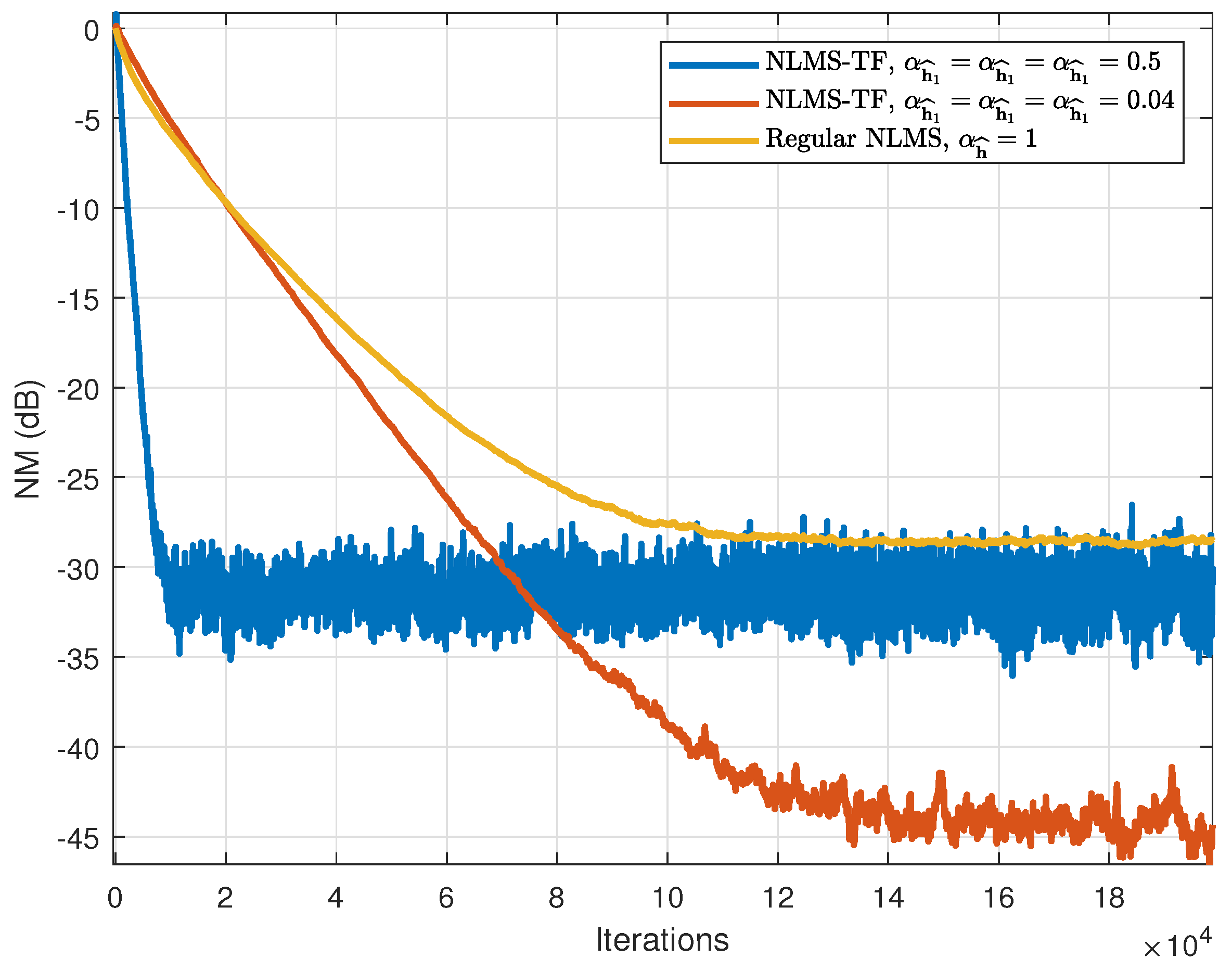
where $e\left(t\right)$ is given in Equation (56). The parameters ${\alpha }_{\widehat{\mathbf{h}}}$ and ${\delta }_{\widehat{\mathbf{h}}}$ represent the normalized step-size parameter and the regularization constant for the global filter, respectively. As previously shown in Reference [9] for bilinear forms, the global misalignment can be controlled by using a constraint on the sum of the normalized step-sizes, and this sum should be smaller than 1. In this way, for different values of ${\alpha }_{{\widehat{\mathbf{h}}}_1}$, ${\alpha }_{{\widehat{\mathbf{h}}}_2}$, ${\alpha }_{{\widehat{\mathbf{h}}}_3}$ fulfilling this condition, the misalignment of the global filter is the same. On the other hand, in the case when ${\alpha }_{{\widehat{\mathbf{h}}}_1}={\alpha }_{{\widehat{\mathbf{h}}}_2}={\alpha }_{{\widehat{\mathbf{h}}}_3}$, the three filters achieve the same level of the misalignment.

Again, we notice that the global impulse response identification involves the use of a filter of length $L_1{L}_2{L}_3$. Because the trilinear approach uses three much shorter impulse responses of lengths $L_1$, $L_2$, and $L_3$, respectively, it is expected that this new solution will yield a faster convergence. This will be shown through simulations.

The NLMS-TF algorithm proposed here is similar to that presented in Reference [19]. However, our choice of the system impulse responses used in simulations is different from that in Reference [19]. On the contrary, we aim to show the performance of the algorithm in a scenario that includes a real echo path. In addition, we also study the tracking capability of the algorithm.

5. Simulation Results

In order to show the performance of our approach, we perform simulations in which we compare the trilinear forms of the proposed algorithms with their regular counterparts.

5.1. Iterative Wiener Filter

In this section, the performance of the proposed iterative Wiener filter for trilinear forms is evaluated in the context of system identification. The input signals that form $\mathcal{X}$$\left(t\right)$ are AR(1) processes, which are obtained by generating white Gaussian noises and then filtering them through a first-order system $1/\left(1-0.9z^{-1}\right)$. The additive noise $v\left(t\right)$, corrupting the output signal $y\left(t\right)$, is white and Gaussian, with the variance set to ${\sigma }_v^2=0.01$. The impulse responses used in simulations are depicted in Figure 1. The impulse response ${\mathbf{h}}_1$ is the first impulse response from the G168 Recommendation [37], of length $L_1=64$ (see Figure 1a). Next, ${\mathbf{h}}_2$ is a random impulse response (with Gaussian distribution) of length $L_2=8$ (as shown in Figure 1b). Finally, the coefficients of the impulse response ${\mathbf{h}}_3$ (depicted in Figure 1c) are evaluated as $h_{3l_3}={0.5}^{l_3-1},l_3=1,2,\dots ,L_3$, using $L_3=4$. Therefore, the global impulse response from Figure 1d results in $\mathbf{h}={\mathbf{h}}_3\otimes {\mathbf{h}}_2\otimes {\mathbf{h}}_1$ and its length is $L=L_1{L}_2{L}_3=2048$. As we can see, this global impulse response is similar (to some extent) to a channel with echoes, similar to an acoustic echo path.

In order to evaluate the identification of the individual filters ${\mathbf{h}}_k,k=1,2,3$, we should use the normalized projection misalignment (NPM) [38]:

$$\begin{array}{ccc}\mathrm{NPM}\left({\mathbf{h}}_k,{\widehat{\mathbf{h}}}_k\right)\hfill & =\hfill & 1-{\left(\frac{{\mathbf{h}}_k^T{\widehat{\mathbf{h}}}_k}{\parallel {\mathbf{h}}_k\parallel \parallel {\widehat{\mathbf{h}}}_k\parallel }\right)}^2,\hfill \end{array}$$

(73)

where $\parallel ·\parallel$ denotes the Euclidean norm. For the identification of the global impulse response, $\mathbf{h}\left(t\right)$, we use the normalized misalignment (NM):

$$\mathrm{NM}\left(\mathbf{h},\widehat{\mathbf{h}}\right)=\frac{\parallel \mathbf{h}-\widehat{\mathbf{h}}{\parallel }^2}{{\parallel \mathbf{h}\parallel }^2}.$$

(74)

We consider that the covariance matrix $\mathbf{R}$ and the cross-correlation vector $\mathbf{p}$ are estimated based on N data samples:

$$\begin{array}{cc}\widehat{\mathbf{R}}\hfill & =\frac{1}{N}\sum _{t=1}^N\mathbf{x}\left(t\right){\mathbf{x}}^T\left(t\right),\hfill \end{array}$$

(75)

$$\begin{array}{cc}\widehat{\mathbf{p}}\hfill & =\frac{1}{N}\sum _{t=1}^N\mathbf{x}\left(t\right)d\left(t\right).\hfill \end{array}$$

(76)

These two terms are a priori computed and they are used afterwards (instead of $\mathbf{R}$ and $\mathbf{p}$) for both the conventional and iterative Wiener filters.

The matrix involved in the linear system, to be solved in the case of the conventional Wiener filter from Equation (19), is of size $L\times L$; hence, a number of data samples larger than L are needed to estimate the statistics in Equations (75) and (76), in order to obtain a good solution. This is shown in Figure 2, where different values of N (that is, the available amount of data in Equations (75) and (76)) are used and the solution provided by the conventional Wiener filter is evaluated for each of these values. Similar to Equation (74), the performance measure in Figure 2 is the NM (in dB), which is defined as $10{\log }_{10}\left({∥\mathbf{h}-{\widehat{\mathbf{h}}}_{\mathrm{W}}∥}^2/{∥\mathbf{h}∥}^2\right)$; in this case, the conventional Wiener solution ${\widehat{\mathbf{h}}}_{\mathrm{W}}$ results from Equation (19) (using Equations (75) and (76)). As we can see, the conventional Wiener filter achieves a reasonable decrease in misalignment only when a large amount of data (i.e., $N>L$) are used to estimate the statistics in Equations (75) and (76).

The main advantage provided by the iterative Wiener filter is that it operates with much shorter filters (due to the decomposition in Equation (20)) and, consequently, the dimensions of the linear systems of equations to be solved are significantly reduced. Therefore, even with a small amount of data (i.e., $N<L$), the iterative Wiener filter is able to obtain a reliable estimation. This advantage is outlined in Figure 3, where the solution provided by the conventional Wiener filter (based on Equation (19) and using Equations (75) and (76)) is compared to the iterative Wiener filter from Equation (42). The performance measure is the NM (in dB), which is evaluated based on Equation (74), for the identification of the global system $\mathbf{h}$. Three amounts of data are considered in this experiment, that is, $N=500,2500,$ and 5000. Clearly, in the first case ($N=500$), the conventional Wiener filter leads to an inaccurate solution due to the small amount of data (as compared to $L=2048$). When the amount of data slightly exceeds the value of L (e.g., $N=2500$), the conventional Wiener filter provides a more reliable solution, that is, the misalignment attenuation is approximately $-10$ dB. Finally, for a large amount of data ($N=5000$), this conventional solution is improved in terms of accuracy (e.g., the misalignment is close to $-20$ dB). On the other hand, in all the previous cases, the proposed iterative Wiener filter achieves a much more accurate solution (with only a few iterations), which outperforms by far the conventional one (even in the case when a small amount of data are available, e.g., $N=500$). For example, the iterative Wiener filter which uses $N=500$ yields a lower misalignment level with respect to the conventional Wiener filter with $N=5000$.

In Figure 4, the performance of the iterative Wiener filter is also illustrated using the NPMs (in dB), based on Equation (73), for the identification of the individual impulse responses from Figure 1a–c. Basically, the same conclusion applies, that is, only a few iterations are required by the iterative Wiener filter to achieve a reliable solution (even for a small amount of data).

5.2. LMS-TF and NLMS-TF

For the second set of simulations, the setup is the same as in the previous experiments. First, we aim to show the influence of the constant step-size values on the performance of the LMS-TF algorithm. The performance in terms of the NM (in dB) is shown in Figure 5.

It can be seen that if the step-sizes take large values, the LMS-TF algorithm reaches convergence after less than ${10}^4$ iterations. Then, as these values decrease, the convergence becomes slower but the steady-state value of the NM also decreases, highlighting the compromise between convergence rate and NM value.

Next, we illustrate the improvement brought by the proposed solution, by comparing the LMS-TF algorithm to its regular counterpart, applied for the identification of the global filter. Figure 6 shows the values of the NM for the regular LMS filter and the LMS-TF. The first observation is that, in order to reach the same steady-state value of the NM, the regular LMS algorithm needs many more iterations. On the other hand, for a similar convergence speed, the final NM provided by the LMS-TF is much lower than that offered by its regular counterpart. This proves that the proposed solution offers a significant improvement with respect to the classical approach.

The next step is to study the behavior of the NLMS-TF filter. First, the performance of the NLMS-TF algorithm is depicted in Figure 7, for different values of the normalized step-sizes. The regularization constants are ${\delta }_{{\widehat{\mathbf{h}}}_1}={\delta }_{{\widehat{\mathbf{h}}}_2}={\delta }_{{\widehat{\mathbf{h}}}_3}=0.001$. The same conclusion as for the LMS-TF case is valid, namely that the decrease in the normalized step-sizes leads to a smaller value of the final NM but at the cost of a slower convergence rate. When the step-size values decrease 10 times, the number of iterations needed to reach convergence increases almost 10 times, while the steady-state NM value decreases by a bit more than 10 dB.

We then compare the NLMS-TF algorithm with its regular counterpart (applied on the global filter) in Figure 8. Again, we observe that the NLMS-TF behaves better than the regular NLMS algorithm, from the perspective of both convergence rate and final NM value.

Finally, the tracking capability of the NLMS-TF algorithm is of interest, that is, the capability of the algorithm to react to abrupt changes to the impulse responses. In order to study this characteristic, we simulated a sudden change of the random impulse response ${\mathbf{h}}_2$ in the middle of the experiment. The results are presented in Figure 9. The improvement brought by the NLMS-TF algorithm is clear. The algorithm tracks faster after the change of the system, while the value of the NM is smaller, as compared to the regular NLMS filter. This proves that even if the environment changes, the proposed approach exhibits good behavior.

6. Conclusions

In this paper, we addressed the problem of multilinear system identification, focusing in particular on trilinear forms in the framework of MISO systems. Trilinear forms are defined with respect to the impulse responses of the system and are treated using third-order tensors. In this context, we derived the corresponding Wiener filter, as well as the LMS and NLMS adaptive algorithms, tailored for such trilinear forms (LMS-TF and NLMS-TF). We have shown through simulations that the proposed algorithms lead to better solutions as compared to their regular counterparts, due to the reformulation of the system identification problem of high dimension in lower dimension problems. Experimental results support the theoretical analysis and highlight the good performance of the proposed solutions for the problem of system identification. Future work can focus on extending the approach to higher-order multilinear systems.

References

1. Roy, R.; Sherman, J. A learning technique for Volterra series representation. IEEE Trans. Autom. Control 1967, 12, 761–764. [Google Scholar] [CrossRef]
2. Barker, H.A.; Obidegwu, S.N.; Pradisthayon, T. Performance of antisymmetric pseudorandom signals in the measurement of 2nd-order Volterra kernels by crosscorrelation. Proc. IEEE 1972, 119, 353–362. [Google Scholar]
3. Annabestani, M.; Naghavi, N.; Nejad, M.M. Nonautoregressive nonlinear identification of IPMC in large deformation situations using generalized Volterra-based approach. IEEE Trans. Instrum. Meas. 2016, 65, 2866–2872. [Google Scholar] [CrossRef]
4. Zhang, Z.; Ma, Y. Modeling of rate-dependent hysteresis using a GPO-based adaptive filter. Sensors 2016, 16, 205. [Google Scholar] [CrossRef]
5. Rugh, W.J. Nonlinear System Theory: The Volterra/Wiener Approach; Johns Hopkins University Press: Baltimore, MD, USA, 1981. [Google Scholar]
6. Carassale, L.; Kareem, A. Modeling nonlinear systems by Volterra series. J. Eng. Mech. 2010, 136, 801–818. [Google Scholar] [CrossRef]
7. Benesty, J.; Paleologu, C.; Ciochină, S. On the identification of bilinear forms with the Wiener filter. IEEE Signal Process. Lett. 2017, 24, 653–657. [Google Scholar] [CrossRef]
8. Bai, E.-W.; Li, D. Convergence of the iterative Hammerstein system identification algorithm. IEEE Trans. Autom. Control 2004, 49, 1929–1940. [Google Scholar] [CrossRef]
9. Paleologu, C.; Benesty, J.; Ciochină, S. Adaptive filtering for the identification of bilinear forms. Digit. Signal Process. 2018, 75, 153–167. [Google Scholar] [CrossRef]
10. Dogariu, L.; Paleologu, C.; Ciochină, S.; Benesty, J.; Piantanida, P. Identification of bilinear forms with the Kalman filter. In Proceedings of the 2018 IEEE International Conference on Acoustics, Speech and Signal Processing (ICASSP), Calgary, AB, Canada, 15–20 April 2018; pp. 4134–4138. [Google Scholar]
11. Dogariu, L.-M.; Ciochină, S.; Paleologu, C.; Benesty, J. A connection between the Kalman filter and an optimized LMS algorithm for bilinear forms. Algorithms 2018, 11, 211. [Google Scholar] [CrossRef]
12. Gesbert, D.; Duhamel, P. Robust blind joint data/channel estimation based on bilinear optimization. In Proceedings of the 8th Workshop on Statistical Signal and Array Processing, Corfu, Greece, 24–26 June 1996; pp. 168–171. [Google Scholar]
13. Stenger, A.; Kellermann, W. Adaptation of a memoryless preprocessor for nonlinear acoustic echo cancelling. Signal Process. 2000, 80, 1747–1760. [Google Scholar] [CrossRef] [Green Version]
14. Ribeiro, L.N.; Schwarz, S.; Rupp, M.; de Almeida, A.L.F.; Mota, J.C.M. A low-complexity equalizer for massive MIMO systems based on array separability. In Proceedings of the 2017 25th European Signal Processing Conference (EUSIPCO), Kos, Greece, 28 August–2 September 2017; pp. 2522–2526. [Google Scholar]
15. Da Costa, M.N.; Favier, G.; Romano, J.M.T. Tensor modelling of MIMO communication systems with performance analysis and Kronecker receivers. Signal Process. 2018, 145, 304–316. [Google Scholar] [CrossRef]
16. Ljung, L. System Identification: Theory for the User, 2nd ed.; Prentice-Hall: Upper Saddle River, NJ, USA, 1999. [Google Scholar]
17. Gay, S.L.; Benesty, J. (Eds.) Acoustic Signal Processing for Telecommunication; Kluwer Academic Publisher: Boston, MA, USA, 2000. [Google Scholar]
18. Benesty, J.; Gaensler, T.; Morgan, D.R.; Sondhi, M.M.; Gay, S.L. Advances in Network and Acoustic Echo Cancellation; Springer: Berlin, Germany, 2001. [Google Scholar]
19. Rupp, M.; Schwarz, S. A tensor LMS algorithm. In Proceedings of the 2015 IEEE International Conference on Acoustics, Speech and Signal Processing (ICASSP), Brisbane, Australia, 19–24 April 2015; pp. 3347–3351. [Google Scholar]
20. Rupp, M.; Schwarz, S. Gradient-based approaches to learn tensor products. In Proceedings of the 2015 23rd European Signal Processing Conference (EUSIPCO), Nice, France, 31 August–4 September 2015; pp. 2486–2490. [Google Scholar]
21. Vervliet, N.; Debals, O.; Sorber, L.; Lathauwer, L.D. Breaking the curse of dimensionality using decompositions of incomplete tensors: Tensor-based scientific computing in big data analysis. IEEE Signal Process. Mag. 2014, 31, 71–79. [Google Scholar] [CrossRef]
22. Sidiropoulos, N.; Lathauwer, L.D.; Fu, X.; Huang, K.; Papalexakis, E.; Faloutsos, C. Tensor decomposition for signal processing and machine learning. IEEE Trans. Signal Process. 2017, 65, 3551–3582. [Google Scholar] [CrossRef]
23. Boussé, M.; Debals, O.; Lathauwer, L.D. A tensor-based method for large-scale blind source separation using segmentation. IEEE Trans. Signal Process. 2017, 65, 346–358. [Google Scholar] [CrossRef]
24. Lathauwer, L.D. Signal Processing Based on Multilinear Algebra. Ph.D. Thesis, Katholieke Universiteit Leuven, Leuven, Belgium, 1997. [Google Scholar]
25. Kolda, T.G.; Bader, B.W. Tensor decompositions and applications. SIAM Rev. 2009, 51, 455–500. [Google Scholar] [CrossRef]
26. Comon, P. Tensors: A brief introduction. IEEE Signal Process. Mag. 2014, 31, 44–53. [Google Scholar] [CrossRef]
27. Cichocki, A.; Mandic, D.P.; Phan, A.H.; Caiafa, C.F.; Zhou, G.; Zhao, Q.; Lathauwer, L.D. Tensor decompositions for signal processing applications. IEEE Signal Process. Mag. 2015, 32, 145–163. [Google Scholar] [CrossRef]
28. Loan, C.F.V. The ubiquitous Kronecker product. J. Comput. Appl. Math. 2000, 123, 85–100. [Google Scholar] [CrossRef] [Green Version]
29. Paleologu, C.; Benesty, J.; Ciochină, S. Linear system identification based on a Kronecker product decomposition. IEEE/ACM Trans. Audio Speech Lang. Process. 2018, 26, 1793–1808. [Google Scholar] [CrossRef]
30. Elisei-Iliescu, C.; Paleologu, C.; Benesty, J.; Stanciu, C.; Anghel, C.; Ciochină, S. Recursive least-squares algorithms for the identification of low-rank systems. IEEE/ACM Trans. Audio Speech Lang. Process. 2019, 27, 903–918. [Google Scholar] [CrossRef]
31. Kiers, H.A.L. Towards a standardized notation and terminology in multiway analysis. J. Chemom. 2000, 14, 105–122. [Google Scholar] [CrossRef]
32. Kroonenberg, P. Applied Multiway Data Analysis; Wiley: Hoboken, NJ, USA, 2008. [Google Scholar]
33. Ribeiro, L.N.; de Almeida, A.L.F.; Mota, J.C.M. Identification of separable systems using trilinear filtering. In Proceedings of the 2015 IEEE 6th International Workshop on Computational Advances in Multi-Sensor Adaptive Processing (CAMSAP), Cancun, Mexico, 13–16 December 2015; pp. 189–192. [Google Scholar]
34. Morgan, D.R.; Kratzer, S.G. On a class of computationally efficient, rapidly converging, generalized NLMS algorithms. IEEE Signal Process. Lett. 1996, 3, 245–247. [Google Scholar] [CrossRef]
35. Haykin, S. Adaptive Filter Theory, 4th ed.; Prentice-Hall: Upper Saddle River, NJ, USA, 2002. [Google Scholar]
36. Benesty, J.; Paleologu, C.; Ciochină, S. On regularization in adaptive filtering. IEEE Trans. Audio Speech Lang. Process. 2011, 19, 1734–1742. [Google Scholar] [CrossRef]
37. Digital Network Echo Cancellers; ITU-T Recommendations G.168; 2002. Available online: https://www.itu.int/rec/T-REC-G.168/en (accessed on 16 April 2019).
38. Morgan, D.R.; Benesty, J.; Sondhi, M.M. On the evaluation of estimated impulse responses. IEEE Signal Process. Lett. 1998, 5, 174–176. [Google Scholar] [CrossRef]
Figure 1. Impulse responses used in simulations: (a) h 1 of length L 1 = 64 (the first impulse response from G168 Recommendation [37]), (b) h 2 of length L 2 = 8 (random impulse response with Gaussian distribution), (c) h 3 of length L 3 = 4 (its elements are evaluated as h 3 l 3 = 0.5 l 3 1 , l 3 = 1 , , L 3 ), and (d) the global impulse response h = h 3 h 2 h 1 of length L = L 1 L 2 L 3 = 2048 .
Symmetry 11 00556 g001
Figure 2. NM of the conventional Wiener filter as a function of the number of available data samples used to estimate the statistics (N), for the identification of the global impulse response from Figure 1d. The input signals are AR(1) processes, L = 2048 , and σ v 2 = 0.01 .
Symmetry 11 00556 g002
Figure 3. NM of the conventional and iterative Wiener filters, for different values of the number of available data samples used to estimate the statistics (N), for the identification of the global impulse response from Figure 1d. The input signals are AR(1) processes, L = 2048 , and σ v 2 = 0.01 .
Symmetry 11 00556 g003
Figure 4. NPM of the iterative Wiener filter, for different values of the number of available data samples used to estimate the statistics (N), for the identification of the individual impulse responses from Figure 1a–c: (a) NPM h 1 , h ^ 1 ( n ) , (b) NPM h 2 , h ^ 2 ( n ) , and (c) NPM h 3 , h ^ 3 ( n ) . The input signals are AR(1) processes, L 1 = 64 , L 2 = 8 , L 3 = 4 , and σ v 2 = 0.01 .
Symmetry 11 00556 g004
Figure 5. NM of the LMS-TF algorithm using different values of the step-size parameters.
Symmetry 11 00556 g005
Figure 6. NM of the LMS-TF and regular LMS algorithms.
Symmetry 11 00556 g006
Figure 7. NM of the NLMS-TF algorithm using different values of the step-size parameters.
Symmetry 11 00556 g007
Figure 8. NM of the NLMS-TF and regular NLMS algorithms.
Symmetry 11 00556 g008
Figure 9. NM of the NLMS-TF and regular NLMS algorithms. The impulse response h 2 changes in the middle of the experiment.
Symmetry 11 00556 g009