Abstract
Shale gas energy is the most prominent and dominating source of power across the globe. The processes for the extraction of shale gas from shale rocks are very complex. In this study, a multiobjective optimization framework is presented for an overall water management system that includes the allocation of freshwater for hydraulic fracturing and optimal management of the resulting wastewater with different techniques. The generated wastewater from the shale fracking process contains highly toxic chemicals. The optimal control of a massive amount of contaminated water is quite a challenging task. Therefore, an on-site treatment plant, underground disposal facility, and treatment plant with expansion capacity were designed to overcome environmental issues. A multiobjective trade-off between socio-economic and environmental concerns was established under a set of conflicting constraints. A solution method—the neutrosophic goal programming approach—is suggested, inspired by independent, neutral/indeterminacy thoughts of the decision-maker(s). A theoretical computational study is presented to show the validity and applicability of the proposed multiobjective shale gas water management optimization model and solution procedure. The obtained results and conclusions, along with the significant contributions, are discussed in the context of shale gas supply chain planning policies over different time horizons.
1. Introduction
Energy sources play a dynamic role in the development, nourishment, and enrichment reputation of any country. Presently, many conventional sources of energy are being used for energy production, but shale gas energy is booming among different energy sources [1,2,3]. Apart from conventional sources of energy, shale gas—which is located within shale rocks—is the most promising source of natural gas. Recently, shale gas has become an emerging source of natural gas across the world [4,5]. The United States is the second-richest country after China in terms of the abundance of shale gas resources. Since the start of this century, significant interest has been shown in the potential extraction of shale gas across the world [6,7,8]. In 2000, only 1% of the US natural gas production was contributed by shale gas energy; by 2010, it was more than 20%, and according to predictions of the US government’s Energy Information Administration (EIA), by 2035 more than 46% of the US’ natural gas supply will be from shale gas [9]. The first extraction of shale gas from shale rocks was done in Fredonia (New York) in 1821 by using shallow and low-pressure fractures. However, horizontal drilling started in the 1930s, and the first well was fractured in the US in 1947. Presently, shale gas potential extraction and enriched abundance in many nations are being investigated. According to Sieminski et al. [10], in 2013, only a few countries (e.g., the US, Canada, and China) have sufficient shale gas enrichment, and future production is planned at commercial scale [10]. China has an apparent strategy to dramatically grow its shale gas production and investment, which has been restricted by its insufficient approach to water, land, and the latest technology. Shale hosts rocks trapping potential shale gas quantities that have numerous common properties, namely, being composed of organic material, a mature petroleum source, containing a high amount of natural gas in the thermogenic gas window spread inside the Earth’s crust where there is high heat and pressure being applied to convert petroleum into natural gas. Most commonly, hydraulic fracturing (also known as fracking) and horizontal drilling are two dominant methods that are being used in the process of shale gas extraction across the world. The high concentration of released toxic and contaminated wastewater from the extraction and use of shale gas affects the environment. A challenge in the shale gas extraction process is preventing environmental pollution. This depends on drilling wells and their capacity, which varies with shale use. Water cannot be reused until a well is fractured and the water starts to withdraw from the well. A study was published by Kerr [11] in May 2011 that strongly suggested shale gas wells contain a rigorous abundance of toxic surface groundwater flows with flammable methane in North-Eastern Pennsylvania. Although the presented study was confined to the contamination of water, the impact in other areas that would be dug out for shale extraction purposes was not discussed.
Over the past few years, various research works have been published suggesting, in the context of optimal production policies, a selection area, supply chain network, and socio-economic balancing during shale gas extraction at the commercial level. Lutz et al. [12] presented a theoretical overview of shale gas development in the context of a more prominent resource-producing country such as the United States. The quantification of shale gas energy and wastewater generation throughout Pennsylvania was revealed with consolidated data obtained from 2189 wells. The concluding remarks were contrary to the current perception regarding the shale gas extraction-to-wastewater evulsion ratio, transportation, disposal facilities, treatment strategies, and the associated factors in the shale gas extraction processes. Yang et al. [13] presented the optimum usage of the water life cycle for drilled well-peds through a discontinuous-time bi-stage stochastic mixed-integer linear programming (SMILP) optimization framework under uncertainty. The model was optimized with a set of long-term historical data. The discussed approach was applied to two Marcellus shale gas uses, which showed the effectiveness of the addressed study. Yang et al. [14] discussed the optimal usage of water in the fracking and drilling mechanism during shale gas extraction processes at commercial scale, and also formulated a new mixed-integer linear programming (MILP) problem that inherently optimizes the capital investment for an optimal shale gas yielding scheme. A case study was implemented in the proposed optimization scenario. Li and Peng [15] investigated a new solution scheme based on interval-valued hesitant fuzzy information for the selection of promising shale gas areas, and discussed the applicability of the proposed approach by selecting the shale gas areas using multi-criteria decision making (MCDM). Although shale gas extraction has been done for over 100 years in two different prominent basins of the United States (i.e., the Appalachian Basin and the Illinois Basin), the wells seldom result in profitable production. The current shale gas extraction process, consisting of horizontal drilling and hydraulic fracturing, has made shale gas synthesis more advantageous.
In April 2012 [16], the cost of extraction incurred over shale gas in different coastal parts of the UK was approximated to be much higher than $200 per barrel, which was compared to oil prices of about $120 per barrel in the UK North Sea. North America has emerged as one of the potential leaders in developing and producing shale energy. In the US and Canada, after the successful economic accomplishment of the Barnett Shale use in Texas, the exploration of promising new sources of shale gas is being made. Gao and You [17] designed an active water cycle configuration for the shale gas extraction process and re-formulated it as a mixed-integer linear fractional programming (MILFP) optimization model under different objectives and sets of constraints. The models were globally optimized using various approaches such as the parametric method, a reformulation linearization approach, the branch and bound method, and the Charnes–Cooper transformation technique. The addressed mathematical models were applied to two case studies based on Marcellus shale play, in which on-site treatment techniques of wastewater gained importance in generating freshwater storage. Sang et al. [18] discussed a numerical optimization model of desorption and adsorption processes for hydraulic fracturing stimulations that was optimized by assuming polar co-ordinate and balance space, respectively. To estimate the receptacle volume of drilled horizontal shale well reservoirs, Gao and You [19] addressed a practical framework for the optimal flow of shale energy networks. The designed configuration comprises various coherent components such as freshwater, shale energy, wastewater management, transportation, and disposal facility with treatment plant options. The formulated models were built in the form of a mixed-integer nonlinear programming (MINLP) problem. The obtained results revealed the trade-off between economic and environmental objectives. Furthermore, Guerra et al. [20] also discussed the mathematical formulation and implementation of a comprehensive shale gas production framework with the integration of the water supply chain management system. The proposed optimization framework was illustrated with two case studies with different leading components of the shale gas production systems. Bartholomew and Mauter [21] also developed a multiobjective mixed-integer linear programming framework to highlight the trade-off between financial cost and human health & environment (HHE) costs in the overall shale gas water management system. The system’s objectives were defined effectively, inherently representing different financial aspects of the shale gas production planning problem. Zhang et al. [22] presented a specific study on shale gas wastewater management systems under uncertainty. The presented optimization framework for shale gas wastewater management system corresponds to the disposal and treatment facilities under the expansion of treatment capacity. The proposed model has been designed by considering fuzzy and stochastic parameters with feasibility degree and probability distribution function at the different significance level. The concluding remarks revealed the optimal wastewater management in cases where underground disposal capacity is scarce. The uncertainty involved in the parameter reduced the reliability risk factor in shale gas production. In the present competitive epoch, different shale-gas-producing countries have motivated the wholesome and challenging study of shale gas production policies and the optimal supply chain network configuration. Lira-Barragán et al. [23] investigated a mathematical programming formulation for integrating water networks consumed for hydraulic fracturing processes in shale gas extraction. The proposed uncertainty pertained to the use of water for a different purpose and highlighted probabilistic aspects. Moreover, the developed models also cover the scheduling problem associated with the whole modeling framework for shale gas extraction. The different expected objective functions were incorporated, which led to the existence of uncertainty in the modeling approach. Interested researchers can find recent publications on shale gas development and future research scope in Chen et al. [24], Knee and Masker [25], Lan et al. [26], Ren et al. [27], Zhang et al. [28], Denham et al. [29], Al-Aboosi and El-Halwagi [30], Jin et al. [31], Ren and Zhang [32], and Wang et al. [33].
Research Gaps and Contribution
Shale gas extraction planning models and optimal strategic implementation inherently depend on various parametric factors that are actively indulged in the decision-making process. The requirement of a tremendous amount of freshwater for hydraulic fracturing (i.e., between 7000 and 40,000 m per well) becomes challenging. The assessment of different freshwater sources is somewhat uneconomic, but other extractions can fulfill freshwater demand. The produced wastewater management system is also an indispensable issue and is very important in shale gas production planning models.
Many recent publications, such as Guo et al. [34], Gao et al. [35], Chebeir et al. [36], Chen et al. [37], Drouven and Grossmann [38], He et al. [39], and Wang et al. [40] have discussed different optimal modeling approaches for shale gas water management systems with socio-economic and environmental concerns. All of the above studies are confined to only uncertain modeling approaches, and have not discussed uncertainty among parameters’ values; however, Zhang et al. [22] incorporated vagueness among parameters and represented it by fuzzy and stochastic quantification methodology. However, the study proposed by Zhang et al. [22] is lagging in two more practical aspects. First, it may not always be possible to have historical data for to the stochastic technique can be applied; additionally, due to some hesitation regarding imprecise parameters, the fuzzy number may not be an appropriate representative of uncertain parameters. Hence, better representation of the degree of hesitation under vagueness or imprecision can be made by using the intuitionistic fuzzy number, which considers the degree of belongingness as well as non-belongingness of the element in the possible set. Second, Zhang et al. [22] only designed the optimization framework for the optimal management of wastewater throughout the shale gas extraction processes, and did not consider the management of freshwater, which is also an integrated part of the whole shale gas extraction over time horizons. Thus, in this study we propose the unification of the two aspects discussed above. The proposed multiobjective shale gas water management system optimization model was designed after considering the most critical aspects of overall water management planning and optimization epoch. Furthermore, the concept of a neutrosophic goal programming approach is new and has not yet been applied in the field of such an emerging source of energy. The proposed model also ensures the trade-off between the socio-economic and environmental effects of shale gas production policies more realistically. The proposed shale gas optimization model also provides an opportunity to adopt the available on-site treatment technology along with the option of expanding the treatment plant, which would be beneficial for Pennsylvania because underground disposal facilities are scarce and most often wastewater is supplied to nearby cities in Ohio. The rest of the paper is summarized as follows:
In Section 2, the methodologies and technical definitions regarding intuitionistic fuzzy parameters and the neutrosophic goal programming approach (NGPA) are discussed, while Section 3 represents the multiobjective shale gas water management optimization model and implementation of the NGPA algorithm. A hypothetical case study is examined in Section 4 that shows the applicability and validity of the proposed approach. Finally, concluding remarks and findings are highlighted based on the present work in Section 5.
2. Methodology
The shale gas optimization and modeling framework discussed in this paper enviably involve significant work-flow procedures. The involvement of various critical terminological aspects in the proposed modeling and computational approach makes the shale gas optimization problem more pervasive. In order to represent these aspects, we have used some technical terminology which is able to define each and every aspect of the proposed model effectively and efficiently. The mathematical technical terminologies used in this study are intuitionistic fuzzy parameters [41,42,43] and those from multiobjective optimization problems [44,45,46] and the neutrosophic goal programming approach, which is based on the neutrosophic decision set (see [47,48,49]). On the basis of these mathematical technical terminologies, we developed an effective modeling and optimization framework for a shale gas water management system that dynamically characterizes the freshwater requirement and the dispensation of the generated wastewater from shale gas wells. The proposed model for shale gas water management systems contemplates different kinds of cost parameters (e.g., acquisition cost, transportation cost, treatment cost, disposal cost, and capital investment) involved in the accumulation process of freshwater and the dispensation of the generated wastewater from the shale gas extraction process. Apart from the cost, different parameters such as the freshwater storage capacity, underground injection disposal capacity of wastewater, wastewater treatment capacity, and the capacity for the expansion of wastewater treatment plants were considered in this study. Moreover, these parameters are not always in deterministic/crisp form, despite containing some kind of ambiguity and vagueness. This ambiguousness and vagueness can be represented by different uncertain parameters, such as fuzzy Zhang et al. [22], intuitionistic fuzzy, stochastic Zhang et al. [22], and other uncertain forms. The fuzzy parameters are only concerned with the maximization of membership degree (belongingness), whereas an intuitionistic fuzzy set is based on more intuition than a fuzzy set, as it deals with the maximization of membership (belongingness) and the minimization of non-membership degree (non-belongingness) of the element in the set. A stochastic parameter involves a probability distribution function with known mean and variances based on the randomly occurring events.
Furthermore, the proposed modeling approach was designed and incorporated with socio-economic and environmental facts. The potential production and distribution of shale gas energy at the commercial level is not a boon unless and until the proper pertinent initiatives are undertaken in order to overcome the by-products released by the shale gas extraction processes. Therefore, the proposed modeling and optimization approach inherently involves more than one objective (known as a multiobjective optimization problem), which is sufficient to justify the trade-off among different critical socio-economic and environmental aspects of shale gas energy. The mathematical formulation of multiple objectives ensures the economic and environmental aspects of shale gas extraction procedures. To deal with the proposed multiobjective shale gas water management optimization model, a neutrosophic goal programming approach was developed that reveals the actual situation more appropriately. The proposed NGPA considers the independent indeterminacy/neutral degree, which is the area of incognizance of a proposition’s value. The selection of the proposed NGPA technique is quite effective, explanatory, and a good representative of real-life situations.
2.1. Intuitionistic Fuzzy Set
Definition 1
([50]). (Intuitionistic fuzzy set (IFS)) Let there be a universal set Y; then, an IFS in Y is given by the ordered triplets as follows:
where
with conditions
where and denote the membership and non-membership functions of the element into the set .
Definition 2
([51] (Intuitionistic fuzzy number)). An intuitionistic fuzzy set of the real number R is said to be an intuitionistic fuzzy number if the following condition holds:
- (i)
- should be intuitionistic fuzzy normal and convex.
- (ii)
- and should be upper and lower semi-continuous functions.
- (iii)
- should be bounded.
Definition 3
([43]). (Triangular intuitionistic fuzzy number) An intuitionistic fuzzy number is said to be a triangular intuitionistic fuzzy number if the membership function and non-membership function are given by:
and
where and is denoted by .
Definition 4
([42]). (Expected interval for intuitionistic fuzzy number) Let us consider that there exists an intuitionistic fuzzy number which belongs to the set of real numbers R with such that . The four functions such that and are non-decreasing and and are non-increasing functions, then the intuitionistic fuzzy number can be represented by membership and non-membership functions stated as follows:
and
Furthermore, Grzegrorzewski [52] discussed the expected interval for the intuitionistic fuzzy number as a crisp interval and presented it as follows:
The lower and upper values of the expected interval for the intuitionistic fuzzy number is defined as given below:
where
Definition 5
([42]). (Expected interval and value for triangular intuitionistic fuzzy number) Suppose that is a triangular intuitionistic fuzzy number with membership and non-membership functions and ; then, the expected interval of the triangular intuitionistic fuzzy number by using the above definition can be obtained as follows:
and
Grzegrorzewski [52] also suggested the expected value for the intuitionistic fuzzy number with the help of lower and upper values of the expected interval. Therefore, the expected value for the triangular intuitionistic fuzzy number is obtained as follows:
Definition 6.
The general mathematical programming formulation of a multiobjective optimization problem with k objectives, j constraints, and q variables can be stated as follows:
where are a set of k different conflicting objectives, are real-valued functions, and are real numbers. is a q-dimensional decision variable vector and X is a feasible solution set.
2.2. Neutrosophic Goal Programming Approach (NGPA)
In the past few decades, the extended version of the fuzzy set (FS) and intuitionistic fuzzy set (IFS) have been introduced. In order to reflect the insightful concept of indeterminacy or neutral thoughts in decision making, a new set called the neutrosophic set was introduced by Smarandache [47]. The technical erm neutrosophic holds two different words, which are neutre derived from French and meaning “neutral”, and sophia, adopted from Greek and meaning “skill” or “wisdom”. Therefore, the word “neutrosophic” concretely means “knowledge of neutral thoughts”. The FS is mainly concerned with the maximization of the degree of belongingness (membership function) of an element in the set, whereas the IFS deals with two aspects, namely, the degree of belongingness (membership function) and the degree of non-belongingness (non-membership function) of the element in the set. The incorporation of the independent neutral/indeterminacy concept in the neutrosophic set differentiates itself from FS and IFS, providing more strength to decision-making processes.
Moreover, many real-life circumstances may not be easy to tackle with only the degree of belongingness and non-belongingness of the element in the set. However, the degree up to some level of belongingness and non-belongingness would be a significant touchstone in the decision-making process. For example, if we take the opinion about the victory of team X in a cricket match, and supposing they have the possible chance of winning equalling 0.8, the chance team X has of losing would be 0.4 and the chance that match would be a tie would be 0.5 (see [53]). All the possibilities are independent of each other and can take any value between 0 and 1. Therefore, this sort of decision-making problem is outside of the domain of FS and IFS, and consequently beyond the periphery of fuzzy programming and intuitionistic fuzzy programming approaches, respectively. Hence, independent indeterminacy conditions under the uncertainty domain are a more technical perspective in real-life optimization problems (see [48,49,53]).
An efficient approach called the neutrosophic goal programming approach (NGPA) based on the neutrosophic decision set [47] was designed in order to reach the best compromise solution of multiobjective optimization problems. The NGPA inherently comprises three membership functions, namely, the maximization of truth and indeterminacy degrees and the minimization of the falsity degree present in any optimization problem. It permits policymakers to manifest independent neutral inferences about decision-making processes and provides an opportunity to effectively reach goals using the NGPA technique.
Definition 7
([47] (Neutrosophic Set)). Let there be a universal discourse Y such that , then a neutrosophic set W in Y is defined by three membership functions, namely, truth , indeterminacy , and falsity , denoted by the following form:
where , and are real standard or non-standard subsets belonging to , also given as, , , and . There is no restriction on the sum of and , so we have
Definition 8
([47]). Let there be two single-valued neutrosophic sets A and B, then with truth , indeterminacy , and falsity membership functions are given by:
- ,
- ,
- for each .
Definition 9
([47]). Let there be two single-valued neutrosophic sets A and B, then with truth , indeterminacy , and falsity membership functions are given by
- ,
- ,
- for each .
The concept of fuzzy decision (D), fuzzy goal (G), and fuzzy constraint (C) was first discussed by [44] and extensively used in many real-life decision-making problems under fuzziness. Therefore, a fuzzy decision set can be defined as follows:
Equivalently, the neutrosophic decision set , with the set of neutrosophic goals and constraints, can be defined as:
where
where , and are the truth, indeterminacy, and falsity membership functions of neutrosophic decision set , respectively.
In order to formulate the different membership functions for multiobjective optimization problems (MOOPs), we defined the bounds for each objective function. The lower and upper bounds for each objective function are represented by and which can be obtained as follows:
First, we solved each objective function as a single objective under the given constraints of the problem. After solving k objectives individually, we have the k solutions set, . After that, the obtained solutions are substituted for each objective function to provide the lower and upper bounds for each objective, as given below:
The bounds for k objective functions under the neutrosophic environment can be obtained as follows:
where and are predetermined real numbers assigned by decision maker(s) (DM(s)). By using the above lower and upper bounds, we defined the linear membership functions under a neutrosophic environment:
In the above case, for all k objective functions. If for any membership , then the value of these memberships will be equal to 1. The diagrammatic representation of the objective function with different components of membership functions under a neutrosophic environment is shown in Figure 1.
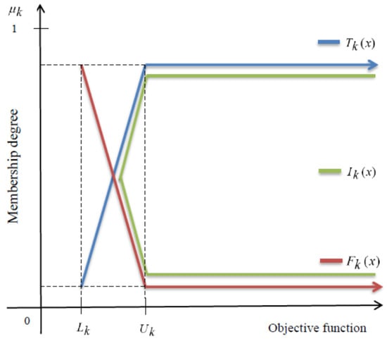
Figure 1.
Diagrammatic representation of truth, indeterminacy, and falsity membership degree for the objective function.
Moreover all the above three discussed membership degrees can be transformed into membership goals according to their respective degrees of attainment. The highest degree of truth membership function that can be achieved is unity (1), the indeterminacy membership function is neutral and independent with the highest attainment degree half (0.5), and the falsity membership function can be achieved with the highest attainment degree zero (0). Now the transformed membership goals under a neutrosophic environment can be expressed as follows:
where , and are the over and under deviations such that , , and for truth membership, indeterminacy membership, and falsity membership goals under a neutrosophic environment.
Intuitionally, the aims are to maximize the truth and indeterminacy membership degrees of neutrosophic objectives and constraints, and minimize the falsity membership degree of neutrosophic objectives and constraints. The general formulation of the neutrosophic goal programming (NGP) model for multiobjective optimization problem (5) is represented as follows:
where , , and are the weights assigned to deviations of the truth, indeterminacy, and falsity membership goals of each objective function, respectively. Now the assignment of corresponding weighting schemes of different weights can be obtained as follows:
, , and .
Hence, the optimum evaluation of multiobjective optimization problems by using the NGP approach is a very useful technique as it involves the degree of indeterminacy, which is independent and certainly ensures the achievement of marginal evaluation of each membership goal by reducing the deviational values under a neutrosophic environment.
3. Shale Gas Water Management System: Modeling and Optimization under Uncertainty
Shale gas is a rapidly emerging and unconventional source of energy found trapped in shale rocks. The extraction process at the wholesale level is very complicated. Since shales usually possess low permeability to permit significant fluid inflow to a well-bore, most shale wells are not adequate sources of natural gas for commercial production. Other sources of natural gases include coal bed methane, methane hydrates, and tight sandstones. Most commonly, the area in which shale gases are trapped are known as resource plays. Shale has comparatively low matrix permeability, which affects gas production at the commercial level and requires the fracturing process to supply permeability. In the past few decades, shale gas has been produced from shale rocks with natural fractures. Shale gas production seems to be booming in recent years due to the latest potential technology in hydraulic fracturing (fracking), which has led in the direction of pervasive artificial fractures around good bores. Horizontal drilling is often used in the shale gas extraction process. Lateral lengths up to 10,000 feet (3000 m) within shale wells are dug out to create maximum borehole surface area in contact with the shale. While injecting water with high pressure into shale rocks, chemicals are added to facilitate the underground fracturing process, which releases natural gas. The fracturing fluid is primarily water and contains approximately 0.5% chemical additives that are fully dissolved into the water. Depending on the size of the area, millions of liters of water are used for fracking, which signifies that thousands of liters of chemicals are injected into the subsurface.
The massive amount of contaminated surface water and groundwater with fracking fluids has emerged as a problematic issue. Generally, accrued shale gas is usually trapped several thousand feet below ground. Different challenging environmental concerns are often observed. For example, methane migration, improper treatment of produced wastewater, and lack of an underground injection disposal site. About 50% to 70% of the injected volume of contaminated water is generated after fracking, and sufficient storage capacity for wastewater management is required. The remaining volume of water remains in the subsurface. The hydraulic fracturing process leads to the perception that it can lead to the contamination of groundwater aquifers. However, foul odors and very toxic local water supply above-ground are also unavoidable truths about shale gas. Acid mine wastewater can be released into groundwater, but it might cause significant contamination of underground freshwater. Usually, the harmful impact and water pollution associated with wastewater and coal production can be reduced to a certain extent in shale gas production. Apart from using water and industrial chemicals, it may also be feasible to frack shale gas with only liquefied propane gas. This extraction option simultaneously reduces water and environmental degradation. It can be implemented in regions like Pennsylvania that have experienced a marginal increment in the freshwater requirement for energy production. More explicitly, shale gas development in the United States represents less than half a percent of total domestic freshwater consumption, although this quantity can reach as high as 25% in particularly arid regions.
Therefore, the proposed shale gas water management strategy has been designed to optimize the allocation of water requirement for different purposes. The designed water supply chain network configuration contains various components, such as the acquisition of freshwater and its transportation, on-site treatment with different technology, underground injection disposal sites, and treatment plants for wastewater with an option for expansion with a to and fro transportation network. Different potential objectives addressing the project planning strategy were also considered in this present study. A well-defined set of dynamic constraints were imposed to represent the modeling approach more realistically. The integrated water flow supply chain network within shale gas planning periods is shown in Figure 2. In Figure 2, the different echelons are presented to highlight the proposed shale gas water management design. The flow of freshwater initiates from different freshwater sources S and is then shipped to various shale sites I. After fracking processes, a possible part of the generated toxic water would be treated by on-site treatment technology O, and the remaining wastewater would be used to dispatch for further management to different treatment plants or disposal sites J, respectively. To enhance the treatment capacity of sewage treatment plants, an opportunity to adopt the different expansion options M was incorporated along with the associated capital investment. Hence, the treated wastewater can be reused for household purposes and in turn can yield significant revenues from the reuse of water. The whole integrated water cycle continues to flow over different time horizons T. Therefore, to assure the optimal flow of water among different echelons, the proposed water flow network captures the actual behavior of flow-back and produced water during shale gas extraction processes. The shale gas project planning model explicitly includes different indices’ set, decision variables, and values of parameters shown in Table 1, which presents the significant characteristic features during the shale gas synthesis process.
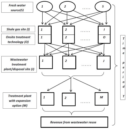
Figure 2.
Representation of shale gas integrated water flow optimization network over time.

Table 1.
Notions and descriptions.
The proposed shale gas water flow network configuration is based on the following assumptions:
- There is no scope for the transportation of water using pipelines throughout the planning horizons.
- The expansion options of underground injection disposal sites have not been considered due to the financial crisis or uneconomic aspects throughout the planning horizons.
- The expansion of the treatment plant has been considered in order to avoid excess wastewater at the subsurface level of underground water during all the planning periods.
- An absolute option of on-site treatment technology has been included that enables the reuse of wastewater within the shale sites throughout the planning horizons.
- The restrictive margin was designed for the minimum and maximum capacity of wastewater treatment by using different on-site treatment technologies throughout the planning horizons.
- The overall produced wastewater volume was successfully managed by the proposed system during all the planning horizons.
3.1. Objective Function
The first objective function is concerned with a different kind of cost incurred over the freshwater. It is quite a challenging task to collect the optimal amount of freshwater directly from natural freshwater sources; however, the option exists to acquire the freshwater from nearby the shale gas plant, which results in a lower acquisition cost. The transportation of freshwater is also required, which again appears as a transportation cost from source s to shale site i over period t, and both are of minimization type. Therefore, the cost function (14) related to freshwater can be furnished as follows:
The second objective mainly focuses on a different kinds of cost levied over the wastewater. It is crucial to manage the huge amount of contaminated or toxic wastewater released during the shale gas energy generation process. The produced amount of wastewater can be handled by either sending it to the treatment plants or by dumping into underground wastewater disposal sites. Both techniques are associated with some cost known as treatment and disposal facility costs, respectively. The transportation of wastewater from shale sites to different treatment plants and disposal sites results in additional transportation costs associated with the wastewater. The total revenues from the reuse of wastewater with some reuse rate are also associated with wastewater from shale site i to disposal and treatment plant j over period t. Therefore, the cost function (15) related to wastewater can be presented as follows:
The third objective function provides the facility of proliferation at treatment plants and underground disposal sites with some predetermined expansion option. The different expansion options require capital investment, which is to be minimized with binary variable taking value 1 if the expansion option m is adopted at treatment plant j over time period t; otherwise 0. Therefore the total capital investment (16) for the expansion of wastewater treatment plant capacity can be summarized as follows:
3.2. Constraints
The constraint given by (17) is related to freshwater demand at shale sites:
At each shale site, a certain quantity of freshwater is required for the hydraulic fracturing process. The total amount of freshwater obtained from different sources is not sufficient to meet the demand at shale sites, but it is indispensable to build up the other sources or by developing other techniques to obtain the freshwater. Therefore on-site treatment technology with a recovery factor for treating wastewater is also an important option to fulfill the demand of such a tremendous amount of freshwater. Hence, the sum of the total amount freshwater acquired from different freshwater sources s and freshwater obtained from various on-site treatment technologies o with the recovery factor for treating wastewater must be greater than or equal to its total requirement at each shale site i over period t:
The constraint has given in (18) is related to the freshwater capacity at each source:
The total amount of freshwater obtained from different sources has some limitations in terms of storage capacity at different sources. The optimal stock of freshwater at different sources may differ marginally. It is necessary to ensure that the total amount of freshwater can be obtained without substantially affecting the storage capacity of each freshwater source. Therefore, the total amount of freshwater acquired from different sources s with the consumption at each shale site i must be less than or equal to its storage capacity at source s over period t:
The constraint given in (19) is related to wastewater capacity at underground disposal sites:
The amount of wastewater generated after the fracturing process contains various toxic chemicals dissolved in it. A proper disposal system with its associated available capacity must be built to overcome fatal environmental effects. Therefore, it must be assured that the amount of wastewater received at different disposal sites can be fully tackled. Thus, the amount of wastewater released from shale site i and received at each disposal site j must be less than or equal to the presumable capacity of each disposal site j over period t:
The constraint given in (20) is related to the wastewater capacity at each treatment plant with its prevalence:
The wastewater treatment facility leads to the option of reusing wastewater. The amount of wastewater liberated from different shale sites restrains the tremendous amount of harmful chemicals that must be treated at the water treatment plant to ensure its reuse for different household purposes. Thus, the amount of wastewater released from different shale sites i and dispatched to different treatment plants j must be less than or equal to the sum of the total capacity of each treatment plant with its several expansion options m over period t:
The constraint given in (21) is related to the overall wastewater capacity at the treatment plant and disposal site:
The total amount of wastewater generated during the shale gas extraction process must be confronted with proper cautionary measures. The option of the treatment plant and disposal site for dealing with wastewater must be sufficient to conquer its harmful effects. Therefore it must be ensured that the total amount of wastewater generated from the hydraulic fracturing process at shale site i is less than or equal to its total capacity at the treatment plant and disposal site j over period t:
The constraint given in (22) is related to different wastewater capacities at the treatment plant and disposal site:
This constraint ensures that regardless of what the excess amount of wastewater released from shale sites is, it must be fully managed by expanding the treatment plant capacity. Therefore, the different treatment plants have a potential storage capacity increment option within the investment costs. Thus, the sum of total wastewater capacity enhanced by expanding treatment plant j with expansion option m, the total capacity of underground disposal and treatment plant j must be less than or equal to the assorted capacity of disposal site and treatment plant j over time period t:
The constraint given in (23) is related to the different wastewater capacities at the treatment plant and disposal site:
The necessity and utilization of a huge amount of freshwater in the whole process of shale gas extraction requires thought regarding its acquisition. Various techniques are used to recycle freshwater. Therefore, one of the most trending techniques is on-site treatment with different technologies. Thus, the reuse specification for hydraulic fracturing with the blending ratio of freshwater to wastewater after the treatment of on-site treatment technology o must be less than or equal to the total amount of freshwater acquired at source s transported to shale site i over period t:
The constraint given in (24) is related to the minimum capacity of the ton-site treatment of wastewater:
This restriction was imposed with the fact that a minimal amount of freshwater must be obtained by using on-site treatment technology. The capital investment towards the setup of on-site treatment plant steers the utilization of on-site treatment technology. Thus, the minimum capacity of on-site wastewater treatment with technology o along with the binary variable taking value one if the certain technology is used (and otherwise 0) at shale site i must be less than or equal to the amount of wastewater treated by on-site treatment technology o over period t:
The constraint given in (25) is related to the maximum capacity of on-site wastewater treatment:
This restriction ensures that the maximal amount of freshwater is acquired by using on-site treatment technology. The upper limit for the on-site treatment of wastewater restricts the excessive holding of wastewater at the on-site treatment plant. Thus, this constraint provides the surety that the minimum capacity of on-site treatment of wastewater with technology o along with the binary variable taking value 1 if the certain technology is used (otherwise 0) at shale site i is greater than or equal to the amount of wastewater treated by on-site treatment technology o over time period t:
The constraint given in (26) is related to the total wastewater produced during the shale gas extraction process:
It must be ensured that the total amount of wastewater generated during the fracking procedures is strictly equal to the sum of different amounts of wastewater distributed to the treatment plant and disposal site. Therefore, the sum of the total amount of wastewater at the treatment plant and disposal site j dispatched from shale site i must be equal to the assorted wastewater capacity at disposal site and treatment plant j over time period t:
The proposed multiobjective shale gas optimization model under uncertainty is presented in model with the fact that parameter values inherently contain vagueness and ambiguousness in the real-life decision-making process. The decision maker(s) or policy maker(s) is(are) not very sure about the exact parameter values due to a lack of proper information, relatively little experience, environmental issues, and other humanitarian logical perception. To overcome these issues, the settings are taken as the triangular intuitionistic fuzzy number and are more elaborately discussed in Section 3.3.
subject to:
where the notation () over different parameters represents the triangular intuitionistic fuzzy number for the indices’ whole set.
3.3. Intuitionistic Fuzzy Parameters
The proposed multiobjective shale gas water management optimization model discussed in Section 3 inherently involves uncertainty or impreciseness. The existence of ambiguity among parameters makes it uncertain. It is not always feasible for decision maker(s) or project manager(s) to assign crisp/exact parameter values. Actual perceptions behind the uncertainty involve a lack of proper information, environmental conditions, the condition of roads, natural calamities, abrupt changes in the prices of fuel, different routes of transportation, shortages of freshwater on sunny days, etc. In such cases, only some vague and inconsistent pieces of information are available regarding the parameter values. Therefore, uncertainty can take different forms, such as fuzzy numbers, stochastic random variables, and other forms of change. Based on this confluent information, one may assume imprecise parameters and easily overcome uncertainty by applying the different techniques to obtain the best estimates of the parameters. In brief, we may distinguish between stochastic and fuzzy methods while dealing with the uncertain dataset. The uncertainty involved in the data due to randomness can be handled with a stochastic programming approach while it can be dealt with using fuzzy techniques due to vagueness or ambiguousness. In the present study, all the parameters were assumed to be triangular intuitionistic fuzzy numbers, which is more realistic as compared to fuzzy numbers as it simultaneously reveals both the degree of belongingness and the degree of non-belongingness. The defuzzification/ranking method of triangular intuitionistic fuzzy parameters is based on the expected interval and expected values of a lower and upper member of the set. Imprecise parameters involved in the different objective functions were converted to their crisp forms by using expected values, whereas uncertain parameters present in constraints were transformed into their deterministic forms using expected intervals. All the pieces of information regarding triangular intuitionistic fuzzy settings used in THE shale gas optimization model are summarized in Table 2.
Table 2.
Information regarding the triangular intuitionistic fuzzy parameters of the shale gas model.
Therefore, the crisp/deterministic version of the proposed multiobjective shale gas water management system optimization model based on the different crisp values of the parameters can be represented in the model as follows:
subject to:
where , , and are the expected value and lower and upper intervals of triangular intuitionistic fuzzy numbers for the entire indices’ set, respectively.
The discussed solution technique (i.e., the neutrosophic goal programming approach (NGPA)) is based on the neutrosophic decision set, which ensures the efficient implementation of the independent neutral thoughts of the decision maker(s). The obtained crisp model can be transformed into to achieve the globally optimal solution of the proposed multiobjective shale gas water management system optimization model.
where , and are the parameter weights assigned to different deviational variables of the neutrosophic membership goals.
3.4. Solution Algorithm
To reformulate the shale gas water management optimization model into the neutrosophic goal programming model, one needs to solve each objective function individually and has to determine the maximum and minimum values of each objective. With the help of these values, the upper and lower bounds for each membership function under a neutrosophic environment were obtained. Then, the truth, indeterminacy, and falsity membership functions for each objective were constructed. The transformation of membership functions into membership goals can be done by using the different deviational variables. The weighting scheme of each aim was designed based on the difference between the best and worst values of the respective objective function. The developed framework for the optimal shale gas water management computational model was transmuted under a neutrosophic environment. The stepwise solution procedures for the proposed neutrosophic goal programming approach can be summarized as follows:
- Step 1.
- Design the proposed multiobjective shale gas water management optimization model as given in .
- Step 2.
- Convert each intuitionistic fuzzy parameter involved in model into its crisp form by using the expected interval and values method as given in Equations (2)–(4) or presented in Table 2.
- Step 3.
- Modify model into and solve model for each objective function individually in order to obtain the best and worst solutions.
- Step 4.
- Determine the upper and lower bounds for each objective function by using Equation (6). Using and , define the upper and lower bounds for truth, indeterminacy, and falsity membership as given in Equations (7)–(9).
- Step 5.
- Transform the truth, indeterminacy, and falsity membership degrees into their respective membership goals and deviational variables as defined in Equations (10)–(12).
- Step 6.
- Formulate the neutrosophic goal programming model defined in and solve the multiobjective shale gas water management optimization model in order to obtain the compromise solution using suitable techniques or some optimization software packages.
4. A Computational Study
The integrated framework representative of the multiobjective shale gas water management optimization model is presented based on a real-life scenario, hypothetical proposition, data, information, and a quick review of the published research (Lutz et al. [12], Rahm and Riha [54], Rahm et al. [55], Zhang et al. [22], Alawattegama [56]). The unified optimal shale gas water planning model was structured to manifest the real-life scenario in the current and future characteristic features of shale gas extraction processes. The proposed model includes the optimal acquisition of freshwater, on-site treatment of wastewater, expansion of treatment plant facility, underground injection disposal site, treatment plant facility, and primary socio-economic concerns and environmental issues with the technical and potential aspects in major shale gas plays in the United States. The acquisition of freshwater from different sources and the inventory holding of freshwater to a certain level for the smooth operation of the shale gas extraction processes is quite a challenging task. Therefore, the acquisition of freshwater is allowed some predetermined budget allocation at the different freshwater sources. The flow-back-produced water from shale play is a matter of grave concern. The privilege of an on-site wastewater treatment facility for reuse purposes at a moderate scale is also feasible and laid down as a base of future technologies. Various burning socio-environmental issues are being raised against the contaminated wastewater generated from shale wells after fracturing processes at the national and international political levels. To overcome these issues, the orientation of wastewater underground disposal sites and treatment facilities with their expansion options have been taken under consideration. There is no scope for pipelines to any extent throughout the shale gas extraction process. All sorts of to and fro flow of freshwater and wastewater have been depicted with roadways. The planning periods are designed in such a way that shale gas production turnover results in an economically profitable scenario.
In this study, the shale gas water management system optimization model comprises one freshwater source, five shale sites with one drilled well at each shale site, and three on-site wastewater treatment facilities. The toxic wastewater management system includes one wastewater underground injection disposal site, two wastewater treatment plants with three expansion options for each treatment plant facility over three planning periods of 5 years each which are capable of representing the whole shale gas production process more realisticallyy. All the summarized parameters were assumed to be a triangular intuitionistic fuzzy number, and their defuzzified version can be obtained from Table 2. The acquisition costs (in $/bbl) of freshwater at source and transportation cost (in $/bbl) of freshwater by road over three planning periods are presented in Table 3. The various costs incurred on account of wastewater, such as transportation cost (in $/bbl) from different shale sites to disposal site and treatment plants, underground injection disposal cost (in $/bbl), and wastewater operational cost at different treatment plants (in $/bbl) over three planning periods are summarized in Table 4. The capital investment costs(in $/bbl) for alternative options for the expansion of treatment plant capacity with the respective enhanced potential volume (in bbl/day) over three planning periods are presented in Table 4. The crisp parameters which include revenues/profits from the reuse of wastewater (in $), reuse rate (in bbl/day), recovery factor for treating wastewater with different treatment technology, and the required ratio of freshwater to sewer for blending after on-site treatment technology, along with the minimum and maximum capacities for on-site treatment with conflicting technology over three time periods are summarized in Table 5. The different restrictive intuitionistic fuzzy parameters (for freshwater and wastewater) were introduced for the optimal allocation of freshwater and wastewater according to their speculated destination. The freshwater acquisition capacity at the source, the requirement of freshwater at different shale sites, the underground wastewater disposal capacity, the wastewater treatment plant capacity, and the overall generated wastewater permitted for managerial purposes are summarized in Table 5. Throughout the project planning scheme, the decision maker(s) or project manager(s) intend to adopt the certainly feasible strategy that ensures the optimal allocation of freshwater and wastewater to their predetermined consumption points. However, during the whole planning periods, the decision maker(s) are confronted with the different multiple conflicting objectives which are to be optimized in order to achieve the global benefits from the production of shale gas energy as well as its commercial distribution. Hence, the proposed multiobjective shale gas water management optimization model experiments with these hypothetical datasets and was applied to tackle the project planning scheme.
Table 3.
Acquisition and transportation costs of freshwater ($/bbl).
Table 4.
Different costs related to wastewater and capital investment for treatment plant expansions ($/bbl).
Table 5.
Capacity restrictions on freshwater and wastewater ( bbl/day).
Results Analyses
The multiobjective shale gas water management optimization model was written in the AMPL language and solved using the BARON solver through NEOS server version 5.0 in the on-line facility provided by Wisconsin Institutes for Discovery at the University of Wisconsin in Madison for solving optimization problems, see Dolan [57], Drud [58], Server [59], and Gropp, W. Moré [60]. The technical description of the problem is presented as follows: The final multiobjective shale gas water management optimization model along with a set of well-defined multiple objectives comprised 219 variables including 42 binary variables, 27 non-linear variables, 150 linear variables, and 336 constraints, including 15 non-linear constraints and 321 linear constraints, 66 equality, and 270 inequality constraints. The total computational time for obtaining the final solution was 0.095 s (CPU time). The proposed multiobjective shale gas water management optimization model was solved with three weight parameters assigned to deviational variables of each membership goal with respect to their marginal membership degree. The first weight parameter was assigned to the truth deviational variable of each membership goal. The second weight parameter was assigned to the indeterminacy deviational variable of each membership goal, and the third weight parameter was assigned to the falsity deviational variable of each membership goal included in all three objective functions. The obtained optimal results were categorized into five main parts: (i) the optimal acquisition of freshwater from various sources to different shale sites in order to ensure smooth operation of the shale gas energy generation system; (ii) prominent emerging technologies for the on-site treatment of wastewater; (iii) the optimal wastewater management system strategy, which is challenging from the environmental point of view; (iv) the optimal expansion plan to enhance the treatment plant capacity; and (v) the optimal values of different conflicting objectives with their corresponding assigned weights. The optimal amounts of freshwater from source to different shale sites are summarized in Table 6. In planning period 1, the amount of freshwater requirements from source to five shale sites were 700.000, 186.765, 700.000, 300.480, and 74.100 bbl/day, respectively. In planning period 2, the requirements of freshwater at each shale site were obtained as 1125.000, 1125.000, 654.419, 131.542 and 212.553 bbl/day, respectively. In planning period 3, the consumption of freshwater at each shale site was 1275.000, 187.613, 528.153, 131.542, and 212.553 bbl/day in order to ensure smooth operation of the shale gas extraction processes. However, with the exception of shale sites 1 and 5, the requirements for freshwater increased for each planning horizon. The maximum requirement of freshwater was in shale site 5 with a volume 1275.000 bbl/day, whereas the minimum freshwater requirement was observed at shale site 1 during planning period 3, with 74.100 bbl/day due to the low and high cost of acquisition and transportation incurred over the amount of freshwater, respectively.
Table 6.
Optimal amount of freshwater and value of objective functions.
The most promising characteristic features of on-site wastewater treatment are the different technologies which are being used to reutilize the wastewater within candidate shale sites. The optimal allocation of wastewater for on-site treatment is summarized in Table 7. The on-site treatment of wastewater by different technologies are emerging options for generating freshwater, which was included in the proposed modeling and optimization framework. At shale site 1, the amount of freshwater after treatment by technology 1 was 150 bbl/day in all three planning horizons; the generation of freshwater after treatment by using technology 2 was 200 bbl/day in each planning period; and by applying technology 3 the values were 1551.71, 2401.65, and 2701.62 bbl/day, which was consistently increasing and ensuring the reuse of wastewater in these three planning horizons. At shale site 2, the amount of freshwater generated by the on-site treatment facility using technology 1 was 127.352 bbl/day in each planning period; the generation of freshwater after treatment using technology 2 was 200, 6250, and 200 bbl/day each; and by applying on-site treatment technology 3 they were 525.313, 4554.66, and 527.01 bbl/day in each planning horizon, respectively. At shale site 3, the amount of freshwater after treatment by technology 1 was 150 bbl/day in all three planning horizons; the generation of freshwater after treatment by using technology 2 was 200 bbl/day in the first and second planning periods, which were the same as shale site 1; whereas it was 2865.32 bbl/day in the third planning slot, and unlike by applying technology 3 the obtained amounts were 1551.71, 2060.51, and 2208.04 in all planning horizons, resulting in a significant increase in the freshwater generation pattern by on-site treatment. At shale site 4, the generation of freshwater using on-site treatment technology 1 was 147.779, 2023.26, and 147.779 bbl/day; by implementing on-site treatment technology 2 they were 200, 272.266, and 730.788 bbl/day, revealing the significant increment in the regenerated wastewater volumes in three planning slots. The amount of freshwater by using on-site treatment technology 3 was 751.275, 300.000, and 300.000 bbl/day in each planning horizon respectively. At shale site 5, the generation of freshwater using on-site treatment technology 1 was 150 bbl/day in each planning slot; by applying on-site treatment technology 2 it was 342.801, 861.73, and 861.73 bbl/day; and after implementing on-site treatment technology 3 it was 300, 860.539, and 860.539 bbl/day in each planning horizon, respectively. Therefore, the optimal regeneration of freshwater at each shale sites was effectively designed by implementing the on-site treatment technology component in the proposed shale gas water management study and could be potentially achieved using these technologies in an efficient manner under many adverse circumstances, especially where wastewater managerial issues are often encountered at the political level.
Table 7.
Optimal amount of wastewater allocation and treatment plant expansion strategy.
The presented wastewater managerial study includes one underground injection disposal site and two treatment plants with its three expansion options which are capable of representing the wastewater management system for the shale plays. Optimal distribution of total wastewater for underground injection disposal and treatment facility is summarized in Table 7. The toxic wastewater produced at shale site 1 was 6.75, 17.25, and 13.25 bbl/day, which is directly transported to the underground injection disposal site; whereas the total volume shipped to the treatment plant was 645, 842.50, and 0 bbl/day in all three time horizons. At shale site 2, the whole volume of wastewater was directly sent to the underground injection disposal site and it was not feasible to facilitate the usage of a treatment plant facility. At shale site 3, a certain volume of wastewater was delivered to an underground injection disposal site and treatment plant 2 without allocating any volume to treatment plant 1. The amount of wastewater shipped to the underground injection disposal site was 6.75, 17.25, and 13.25 bbl/day, and the optimal allocations to treatment plant 1 were 137.71, 675, and 850 bbl/day in the three planning periods. At shale sites 4 and 5, the overall volume of produced wastewater that would be delivered from both shale sites were the same and found to be 6.75, 17.25, and 13.25 bbl/day for underground injection disposal purposes: 645, 842.50, and 937.50 bbl/day towards treatment plant 1 whereas the optimal shipment volumes of wastewater from both shale sites to treatment plant 2 were 137.71, 675, and 850 bbl/day in all three planning horizons, respectively. The optimal allocation strategy for the total wastewater volumes was described in such a fashion that the optimal contribution of each wastewater management system components had equal significance. At all five shale sites, the generated amount of wastewater sent from each shale site to the underground injection disposal site were 6.75, 17.25, and 13.25 bbl/day over the three planning horizons, respectively, revealing the maximum permitted amount at the underground injection disposal site and restraining the subsurface water for a certain period. More elaborately, it could be concluded that during the various time horizons it was not found optimal and feasible to flow the wastewater towards the underground injection disposal site due to the significant cost of transportation and the underground injection disposal facility. At shale site 1, the amount of wastewater that would be shipped to treatment plant 1 was 645 and 842.50 bbl/day for planning horizons 1 and 2, respectively. The shipment of wastewater from shale site 1 to treatment plant 2 was not found to be feasible due to the significant increase in the transportation cost incurred over wastewater. At shale site 2, the allocation of any wastewater amount to treatment plants 1 and 2 was not found to be justified in all three planning periods. At shale site 3, it was not feasible to deliver any amount of wastewater to treatment plant 1 during all three planning periods, although the amount of wastewater that would be shipped to treatment plant 2 was 137.71, 675, and 850 bbl/day in the three planning horizons, respectively. At shale sites 4 and 5, the volume of wastewater that would be delivered from both shale sites were the same and found to be 645, 842.50, and 937.5 bbl/day towards treatment plant 1, whereas the optimal shipment volume of wastewater from both shale sites to treatment plant 2 were 137.71, 675, and 850 bbl/day in all three planning horizons respectively.
During all three planning horizons, treatment plant expansion options played a significant role in dealing with the excess volume of wastewater produced at different shale sites. The vital dominant characteristic of treatment plant expansion was mainly due to limited and rare existence of underground injection disposal site facilities in some places. The limitations imposed on underground injection disposal sites enabled the expanded scope of treatment plant expansions. The optimal strategy for the expansion of treatment plants is presented in Table 7. The optimal expansion results of treatment plant 1 during planning periods 1 and 3 by using expansion option 1 were 600 bbl/day each. By using expansion option 2 in planning periods 1 and 3, the optimal capacity was 750 bbl/day each; and by using expansion option 3 in planning periods 1 and 3, the optimal capacity was 850 bbl/day each. There was no need to expand the treatment capacity of treatment plant 1 in planning period 2. Moreover, the optimal expansion strategy for treatment plant 2 by using all three expansion options during planning horizon 1 were obtained as 550, 650, and 850 bbl/day, whereas in planning period 2, only expansion option 2 was suggested to enhance the treatment capacity. There was no more optimal strategy indicated for the rest of the expansion options. The compromise solution results obtained by solving the proposed multiobjective shale gas water management model are summarized in Table 6. The minimum total cost of acquisition and transportation of freshwater at the source and from different sources to shale sites was USD $525126.00, whereas the net cost incurred over the entire amount of wastewater management during the three planning periods was obtained as USD $4025940.00. The optimal strategy to expand the treatment plant capacity with the predetermined expansion option was presented efficiently and the total capital investment levied on the expansion of the wastewater treatment plant was USD $5548.97, which reveals that there is still adequate opportunity to expand the capacity of the treatment plant. Shale gas water management systems play an important role in the whole process of generating shale gas energy. The acquisition of a huge amount of freshwater for the fracturing process is a challenging task. The wastewater released from shale sites is toxic in nature and contains various harmful dissolved elements. Therefore, a well-organized wastewater management system includes disposal sites (underground injections) and the establishment of different treatment plants with expansion options.
The overall shale gas water modeling approach was presented, inevitably revealing more practical aspects of decision-making scenarios. Uncertainty among parameters due to vagueness and hesitation were addressed with the triangular intuitionistic fuzzy number, which complies over the degree of acceptance and non-acceptance simultaneously. For example, if the decision maker intends to quantify the value of freshwater requirement with some estimated value, such as each shale site requires approximately 54,800 bbl/day for fracking and horizontal drilling purposes, then the most likely estimated interval would be 54,750–54,850 bbl/day, along with some hesitation degree that may be given as 54,700–54900 bbl/day, which ensures less violation of risks with degree of acceptance and non-acceptance. The representation of different constraints imposed over various parameters also reflects the real scenario of Pennsylvania. In Pennsylvania, underground disposal facilities are very rare and most often wastewater is shipped to nearby cities in Ohio. The solution results have shown a similar situation, and less sewage has been allocated to a different underground disposal facility. Furthermore, the scope for on-site treatment technology and expansion capacity options of treatment plants have been optimally utilized. The resulting optimal allocation of wastewater for on-site treatment at different shale sites shows another advantage by reducing the transportation cost incurred over the treatment and disposal facilities. The opportunity for the expansion capacity option of the treatment plant—if needed—was propounded, and results show that some expansion option was adopted due to the lesser capital investment. The determination of the wastewater reuse rate at the treatment plant also yielded a significant amount of freshwater generation and ensured a lesser burden on the underground disposal facility, which again exhibits substantial characteristic features of the shale gas modeling approach of Pennsylvania. Thus, the proposed shale gas water management model can be easily applied to shale gas energy project planning problems that inherently involve uncertain parameters. The decision maker(s) or project manager(s) can conclusively determine the optimal allocation of each water component with a set of multiple conflicting objectives along with a profitable and economic strategy.
5. Conclusions
The multiobjective shale gas water management optimization model addressed within synthesizes the optimum allocation of water resources for shale gas extraction processes. It assures the optimal distribution of freshwater and wastewater, which are the complementary components of shale gas energy production problems. The proposed shale gas modeling outlook is reliable and provides a helpful tool to investigate and analyze the trade-off between socio-economic and environmental concerns globally. The different costs incurred over freshwater, charges levied on wastewater, and capital investment of expanding treatment plant capacity along with the set of shale gas water management system constraints were optimized simultaneously. Uncertainty measures were incorporated among different parameters to demonstrate the actual situations encountered in real-life shale gas optimization frameworks. The accumulation of freshwater from various sources is a crucial task to fulfill commercial needs. However, alternate options were suggested for the generation of freshwater by using on-site treatment technology, which simultaneously reduced the transportation costs for freshwater. Underground injection disposal sites and treatment plant facilities are two major consumption points of generated wastewater from shale sites. A critical factor in the reuse of water in shale gas is the detailed coordination of activities. For greater convenience, auxiliary options have also been introduced to tackle the excess amount of wastewater in the form of on-site treatment technology and different potential expansions of treatment plant capacity at each shale site during each planning horizon. Unlike the various existing conventional solution techniques, the neutrosophic goal programming approach was suggested, which also considers the independent neutral thoughts of decision makers in the decision-making process. Since the proposed approach was applied to a small-scale shale gas extraction process (see Figure 2), it resulted in the globally optimal solution for all objectives simultaneously. However, it may not always be possible to have a globally optimal solution when dealing with large-scale dataset problems. The discussed approach cannot capture the stochastic nature of parameters, which consequently cannot be applied to stochastic optimization problems.
The significant contributions of the proposed multiobjective shale gas water management system are summarized as follows:
- The proposed study considers the overall shale gas water management system which consists of freshwater acquisition at sources, on-site wastewater treatment facilities at each shale site, underground injection disposal sewage facilities, different treatment plant options for the reuse of wastewater and the total wastewater capacity which are feasible to handle without affecting the environmental issues. The decision maker(s) or project manager(s) may adopt the presented shale gas modeling framework, which has a magnetic orientation concerning the overall water management system. However, pipeline facilities have not been included throughout the shale gas energy extraction due to their uneconomic aspect.
- Uncertainty among the parameter values is commonly known in the decision-making process. In this shale gas optimization model, the different parameters (e.g., acquisition cost, transportation cost, treatment cost, disposal cost, and capital investment) are taken as the triangular intuitionistic fuzzy number, which is based on more intuition and leads to more realistic uncertainty modeling texture. It also ensures that the system costs the reliability of each component (costs related to freshwater and wastewater) more realistically. The crisp versions of uncertain parameters were determined in terms of expected interval and expected values.
- A neutrosophic-based computational decision-making algorithm for such a complex and dynamic multiobjective shale gas water management optimization model provides benefits while obtaining globally optimal solutions. The indeterminacy/neutral thought is the region of the propositions’ value uncertainly and originates from the independent and impartial thoughts. Therefore, the proposed NGPA is a dominating and suitable conventional optimization technique that is preferred over others due to the existence of its independent indeterminacy degree.
- The multiobjective shale gas project planning model was implemented with a possible dataset and the obtained optimal results were analyzed for each component of the shale gas system in a well-organized and efficient manner. Hence, it was concluded that the proposed optimal strategy for shale gas production could be adopted for more sophisticated and quite typical Marcellus shale plays in large-scale long-term scenarios.
Due to manuscript drafting constraints and space limitations, some important aspects remain untouched and may be explored as a future research scope. The presented shale gas water management modeling approach could be extended by considering different essential aspects such as the to and fro movement of water through the pipeline which was not considered in this paper. The presented computational study was demonstrated for small-scale shale-plays, which could be further explored for large-scale and long-term time horizons by enhancing the number of shale sites and different sources of freshwater and various destinations for wastewater.
Flow-back water does not exit instantaneously, but follows a decline curve. Most of the water exits in the first 3–4 weeks, but there is small and a continuous flow of produced water during all the shale-sites life. Therefore the presented modeling approach may be extended by capturing the above-discussed behavior of flow-back produced water. On-site treatment technology exerts less pressure on the underground disposal of wastewater and provides an opportunity to reuse the treated wastewater for fracking purposes within the shale sites itself. If there are no NORMs (normally occurring radioactive materials), the most costly part of water treatment is desalination. Therefore, the sort of on-site treatment technologies may be specified along with their actual cost, and the possibility of being used for on-site treatment purposes may be explored as a future study. Most of the water management system (e.g., the water treated in municipal wastewater treatment facilities that are usually not prepared to deal with hypersaline water) are presently forbidden and may be implemented and executed by including them under a good practices scheme in future work. From the decision-making point of view, hierarchical decision-making processes could be adopted, ensuring a decentralized decision-making scenario and providing more flexibility compared to multiobjective optimization techniques with a single decision maker. Apart from conventional solution techniques, some metaheuristic algorithms could be applied to solve such shale gas water management planning problems. Furthermore, the propounded neutrosophic modeling approach could be applied to real-life dataset problems such as supplier selection problems, inventory control problems, supply chain management, humanitarian logistic problems, etc. The proposed approach could be further extended by incorporating the multi-choice and stochastic parameters along with bi-level and multi-level decision-making scenarios.
Author Contributions
Conceptualization, F.A. and A.Y.A.; methodology, F.A.; formal analysis, A.Y.A.; writing—original draft preparation, F.A.; writing—review and editing, F.A.; supervision, A.Y.A.; project administration, F.S.; funding acquisition, F.S.
Funding
This research received no external funding.
Acknowledgments
All authors are deeply thankful to potential reviewers and editors for their valuable suggestions to improve the quality and readability of the manuscript.
Conflicts of Interest
The authors declare no conflict of interest.
References
- Zoback, M.D.; Arent, D.J. Shale gas: Development opportunities and challenges. In Proceedings of the 5th Asian Mining Congress, Kolkata, India, 13–15 February 2014; Volume 44. [Google Scholar]
- Moniz, E.J.; Jacoby, H.D.; Meggs, A.J.; Armtrong, R.; Cohn, D.; Connors, S.; Deutch, J.; Ejaz, Q.; Hezir, J.; Kaufman, G. The Future of Natural Gas; Massachusetts Institute of Technology: Cambridge, MA, USA, 2011. [Google Scholar]
- Shaffer, D.L.; Arias Chavez, L.H.; Ben-Sasson, M.; Romero-Vargas Castrillon, S.; Yip, N.Y.; Elimelech, M. Desalination and reuse of high-salinity shale gas produced water: drivers, technologies, and future directions. Environ. Sci. Technol. 2013, 47, 9569–9583. [Google Scholar] [CrossRef]
- Asche, F.; Oglend, A.; Osmundsen, P. Gas versus oil prices the impact of shale gas. Energy Policy 2012, 47, 117–124. [Google Scholar] [CrossRef]
- Wenzhi, Z.; Dazhong, D.; Jianzhong, L.; Guosheng, Z. The resource potential and future status in natural gas development of shale gas in China. Eng. Sci. 2012, 14, 46–52. [Google Scholar]
- Vengosh, A.; Jackson, R.B.; Warner, N.; Darrah, T.H.; Kondash, A. A critical review of the risks to water resources from unconventional shale gas development and hydraulic fracturing in the United States. Environ. Sci. Technol. 2014, 48, 8334–8348. [Google Scholar] [CrossRef]
- Vidic, R.D.; Brantley, S.L.; Vandenbossche, J.M.; Yoxtheimer, D.; Abad, J.D. Impact of shale gas development on regional water quality. Science 2013, 340, 1235009. [Google Scholar] [CrossRef]
- Warner, N.R.; Christie, C.A.; Jackson, R.B.; Vengosh, A. Impacts of shale gas wastewater disposal on water quality in western Pennsylvania. Environ. Sci. Technol. 2013, 47, 11849–11857. [Google Scholar] [CrossRef]
- Stevens, P. The Shale Gas Revolution: Developments and Changes; Chatham House: London, UK, 2012. [Google Scholar]
- Sieminski, A. International energy outlook. In Proceedings of the Deloitte Oil and Gas Conference, Houston, TX, USA, 18 November 2014. [Google Scholar]
- Kerr, R.A. Study: High-Tech Gas Drilling Is Fouling Drinking Water. Science 2011, 332, 775. [Google Scholar]
- Lutz, B.D.; Lewis, A.N.; Doyle, M.W. Generation, transport, and disposal of wastewater associated with Marcellus Shale gas development. Water Resour. Res. 2013, 49, 647–656. [Google Scholar] [CrossRef]
- Yang, L.; Grossmann, I.E.; Manno, J. Optimization models for shale gas water management. AIChE J. 2014, 60, 3490–3501. [Google Scholar] [CrossRef]
- Yang, L.; Grossmann, I.E.; Mauter, M.S.; Dilmore, R.M. Investment optimization model for freshwater acquisition and wastewater handling in shale gas production. AIChE J. 2015, 61, 1770–1782. [Google Scholar] [CrossRef]
- Li, L.G.; Peng, D.H. Interval-valued hesitant fuzzy Hamacher synergetic weighted aggregation operators and their application to shale gas areas selection. Math. Probl. Eng. 2014, 2014, 181050. [Google Scholar] [CrossRef]
- Gloyston, H.; Johnstone, C. UK Has Vast Shale Gas Reserves, Geologists Say. 2012. Available online: https://www.birmingham.ac.uk/Documents/research/SocialSciences/NuclearEnergyFullReport.pdf (accessed on 16 March 2019).
- Gao, J.; You, F. Optimal design and operations of supply chain networks for water management in shale gas production: MILFP model and algorithms for the water-energy nexus. AIChE J. 2015, 61, 1184–1208. [Google Scholar] [CrossRef]
- Sang, Y.; Chen, H.; Yang, S.; Guo, X.; Zhou, C.; Fang, B.; Zhou, F.; Yang, J. A new mathematical model considering adsorption and desorption process for productivity prediction of volume fractured horizontal wells in shale gas reservoirs. J. Nat. Gas Sci. Eng. 2014, 19, 228–236. [Google Scholar] [CrossRef]
- Gao, J.; You, F. Shale gas supply chain design and operations toward better economic and life cycle environmental performance: MINLP model and global optimization algorithm. ACS Sustain. Chem. Eng. 2015, 3, 1282–1291. [Google Scholar] [CrossRef]
- Guerra, O.J.; Calderón, A.J.; Papageorgiou, L.G.; Siirola, J.J.; Reklaitis, G.V. An optimization framework for the integration of water management and shale gas supply chain design. Comput. Chem. Eng. 2016, 92, 230–255. [Google Scholar] [CrossRef]
- Bartholomew, T.V.; Mauter, M.S. Multiobjective optimization model for minimizing cost and environmental impact in shale gas water and wastewater management. ACS Sustain. Chem. Eng. 2016, 4, 3728–3735. [Google Scholar] [CrossRef]
- Zhang, X.; Sun, A.Y.; Duncan, I.J. Shale gas wastewater management under uncertainty. J. Environ. Manag. 2016, 165, 188–198. [Google Scholar] [CrossRef] [PubMed]
- Lira-Barragán, L.F.; Ponce-Ortega, J.M.; Serna-González, M.; El-Halwagi, M.M. Optimal reuse of flowback wastewater in hydraulic fracturing including seasonal and environmental constraints. AIChE J. 2016, 62, 1634–1645. [Google Scholar] [CrossRef]
- Chen, Y.; He, L.; Guan, Y.; Lu, H.; Li, J. Life cycle assessment of greenhouse gas emissions and water-energy optimization for shale gas supply chain planning based on multi-level approach: Case study in Barnett, Marcellus, Fayetteville, and Haynesville shales. Energy Convers. Manag. 2017, 134, 382–398. [Google Scholar] [CrossRef]
- Knee, K.L.; Masker, A.E. Association between unconventional oil and gas (UOG) development and water quality in small streams overlying the Marcellus Shale. Freshw. Sci. 2019, 38, 113–130. [Google Scholar] [CrossRef]
- Lan, Y.; Yang, Z.; Wang, P.; Yan, Y.; Zhang, L.; Ran, J. A review of microscopic seepage mechanism for shale gas extracted by supercritical CO2 flooding. Fuel 2019, 238, 412–424. [Google Scholar] [CrossRef]
- Ren, K.; Tang, X.; Jin, Y.; Wang, J.; Feng, C.; Höök, M. Bi-objective optimization of water management in shale gas exploration with uncertainty: A case study from Sichuan, China. Resour. Conserv. Recycl. 2019, 143, 226–235. [Google Scholar] [CrossRef]
- Zhang, Y.; Clark, A.; Rupp, J.A.; Graham, J.D. How do incentives influence local public support for the siting of shale gas projects in China? J. Risk Res. 2019. [Google Scholar] [CrossRef]
- Denham, A.; Willis, M.; Zavez, A.; Hill, E. Unconventional natural gas development and hospitalizations: Evidence from Pennsylvania, United States, 2003–2014. Public Health 2019, 168, 17–25. [Google Scholar] [CrossRef]
- Al-Aboosi, F.; El-Halwagi, M. An integrated approach to water-energy nexus in shale-gas production. Processes 2018, 6, 52. [Google Scholar] [CrossRef]
- Jin, L.; Fu, H.; Kim, Y.; Wang, L.; Cheng, H.; Huang, G. The α-Representation Inexact T2 Fuzzy Sets Programming Model for Water Resources Management of the Southern Min River Basin under Uncertainty. Symmetry 2018, 10, 579. [Google Scholar] [CrossRef]
- Ren, C.; Zhang, H. A Fuzzy Max–Min Decision Bi-Level Fuzzy Programming Model for Water Resources Optimization Allocation under Uncertainty. Water 2018, 10, 488. [Google Scholar] [CrossRef]
- Wang, H.; Zhang, C.; Guo, P. An Interval Quadratic Fuzzy Dependent-Chance Programming Model for Optimal Irrigation Water Allocation under Uncertainty. Water 2018, 10, 684. [Google Scholar] [CrossRef]
- Guo, M.; Lu, X.; Nielsen, C.P.; McElroy, M.B.; Shi, W.; Chen, Y.; Xu, Y. Prospects for shale gas production in China: Implications for water demand. Renew. Sustain. Energy Rev. 2016, 66, 742–750. [Google Scholar] [CrossRef]
- Gao, J.; He, C.; You, F. Shale Gas Process and Supply Chain Optimization. In Advances in Energy Systems Engineering; Springer: Cham, Switzerland, 2017; pp. 21–46. [Google Scholar]
- Chebeir, J.; Geraili, A.; Romagnoli, J. Development of Shale Gas Supply Chain Network under Market Uncertainties. Energies 2017, 10, 246. [Google Scholar] [CrossRef]
- Chen, Y.; He, L.; Li, J.; Zhang, S. Multi-criteria design of shale-gas-water supply chains and production systems towards optimal life cycle economics and greenhouse gas emissions under uncertainty. Comput. Chem. Eng. 2018, 109, 216–235. [Google Scholar] [CrossRef]
- Drouven, M.G.; Grossmann, I.E. Mixed-integer programming models for line pressure optimization in shale gas gathering systems. J. Pet. Sci. Eng. 2017, 157, 1021–1032. [Google Scholar] [CrossRef]
- He, L.; Chen, Y.; Li, J. A three-level framework for balancing the tradeoffs among the energy, water, and air-emission implications within the life-cycle shale gas supply chains. Resour. Conserv. Recycl. 2018, 133, 206–228. [Google Scholar] [CrossRef]
- Wang, J.; Liu, M.; Bentley, Y.; Feng, L.; Zhang, C. Water use for shale gas extraction in the Sichuan Basin, China. J. Environ. Manag. 2018, 226, 13–21. [Google Scholar] [CrossRef] [PubMed]
- Ye, J. Expected value method for intuitionistic trapezoidal fuzzy multicriteria decision-making problems. Expert Syst. Appl. 2011, 38, 11730–11734. [Google Scholar] [CrossRef]
- Nishad, A.K.; Singh, S.R. Solving multi-objective decision making problem in intuitionistic fuzzy environment. Int. J. Syst. Assur. Eng. Manag. 2015, 6, 206–215. [Google Scholar] [CrossRef]
- Singh, S.K.; Yadav, S.P. Intuitionistic fuzzy non linear programming problem: Modeling and optimization in manufacturing systems. J. Intell. Fuzzy Syst. 2015, 28, 1421–1433. [Google Scholar]
- Bellman, R.E.; Zadeh, L.A. Decision-Making in a Fuzzy Environment. Manag. Sci. 1970, 17, B-141–B-146. [Google Scholar] [CrossRef]
- Zadeh, L. Fuzzy sets. Inf. Control 1965, 8, 338–353. [Google Scholar] [CrossRef]
- Zimmermann, H.J. Description and optimization of fuzzy systems. Int. J. Gen. Syst. 1976, 2, 209–215. [Google Scholar] [CrossRef]
- Smarandache, F. A Unifying Field in Logics: Neutrosophic Logic. In Philosophy; American Research Press(APP): Rehoboth, NM, USA, 1999; pp. 1–141. [Google Scholar]
- Ahmad, F.; Adhami, A.Y. Neutrosophic programming approach to multiobjective nonlinear transportation problem with fuzzy parameters. Int. J. Manag. Sci. Eng. Manag. 2018. [Google Scholar] [CrossRef]
- Ahmad, F.; Adhami, A.Y.; Smarandache, F. Single Valued Neutrosophic Hesitant Fuzzy Computational Algorithm for Multiobjective Nonlinear Optimization Problem. Neutrosophic Sets Syst. 2018, 22. [Google Scholar] [CrossRef]
- Atanassov, K.T. Intuitionistic fuzzy sets. Fuzzy Sets Syst. 1986, 20, 87–96. [Google Scholar] [CrossRef]
- Ebrahimnejad, A.; Verdegay, J.L. A new approach for solving fully intuitionistic fuzzy transportation problems. Fuzzy Optim. Decis. Mak. 2018, 17, 447–474. [Google Scholar] [CrossRef]
- Grzegrorzewski, P. The hamming distance between intuitionistic fuzzy sets. In Proceedings of the 10th IFSA world congress, Istanbul, Turkey, 30 June–2 July 2003; Volume 30, pp. 35–38. [Google Scholar]
- Rizk-Allah, R.M.; Hassanien, A.E.; Elhoseny, M. A multi-objective transportation model under neutrosophic environment. Comput. Electr. Eng. 2018, 69, 705–719. [Google Scholar] [CrossRef]
- Rahm, B.G.; Riha, S.J. Toward strategic management of shale gas development: Regional, collective impacts on water resources. Environ. Sci. Policy 2012, 17, 12–23. [Google Scholar] [CrossRef]
- Rahm, B.G.; Bates, J.T.; Bertoia, L.R.; Galford, A.E.; Yoxtheimer, D.A.; Riha, S.J. Wastewater management and Marcellus Shale gas development: Trends, drivers, and planning implications. J. Environ. Manag. 2013, 120, 105–113. [Google Scholar] [CrossRef]
- Alawattegama, S.K. Survey of Well Water Contamination in a Rural Southwestern Pennsylvania Community with Unconventional Shale Gas Drilling. Ph.D. Thesis, Duquesne University, Pittsburgh, PA, USA, 2013. [Google Scholar]
- Dolan, E. The Neos Server 4.0 Administrative Guide; Technical Report; Memorandum ANL/MCS-TM-250; Mathematics and Computer Science Division, Argonne National Laboratory: Argonne, IL, USA, 2001.
- Drud, A.S. CONOPT—A large-scale GRG code. ORSA J. Comput. 1994, 6, 207–216. [Google Scholar] [CrossRef]
- Server, N. State-of-the-Art Solvers for Numerical Optimization. 2016. Available online: https://neos-server.org/neos/ (accessed on 16 March 2019).
- Gropp, W.; Moré, J. Optimization environments and the NEOS server. In Approximation Theory and Optimization; Cambridge University Press: Cambridge, UK, 1997; pp. 167–182. [Google Scholar]
© 2019 by the authors. Licensee MDPI, Basel, Switzerland. This article is an open access article distributed under the terms and conditions of the Creative Commons Attribution (CC BY) license (http://creativecommons.org/licenses/by/4.0/).