NHPP Software Reliability Model with Inflection Factor of the Fault Detection Rate Considering the Uncertainty of Software Operating Environments and Predictive Analysis

Abstract
:1. Introduction
2. NHPP Software Reliability Modeling
2.1. A General NHPP Software Reliability Model
2.2. A New NHPP Software Reliability Model
3. Parameter Estimation and Criteria for Model Comparisons
3.1. Parameter Estimation and Models for Comparison
3.2. Criteria for Model Comparison
3.3. Confidence Interval
4. Numerical Examples
4.1. Data Information
4.2. Results of the Estimated Parameters
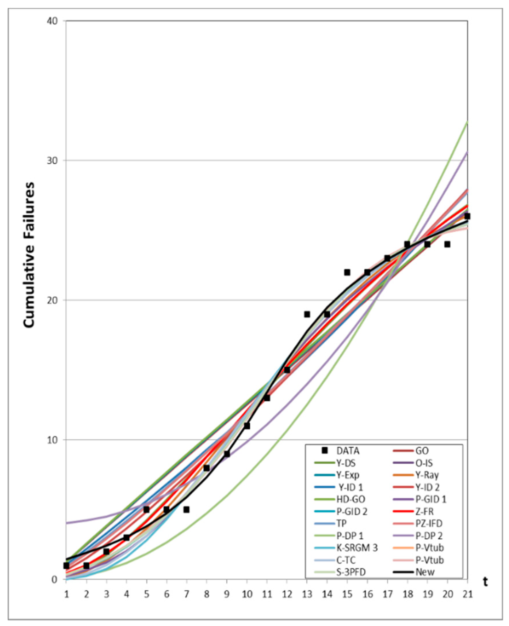
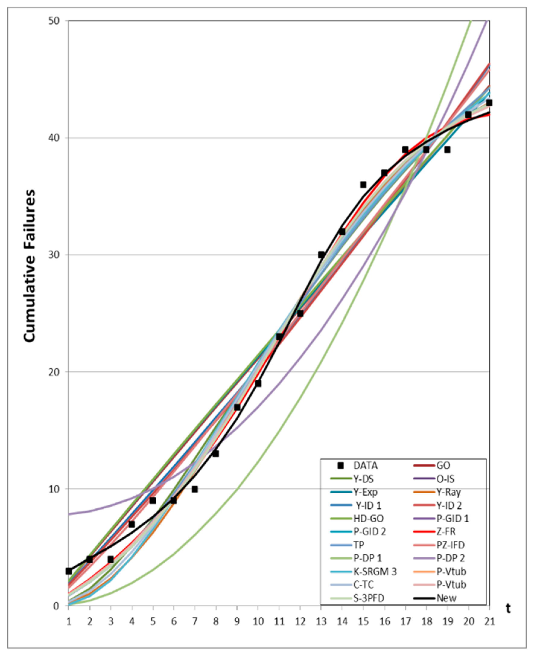
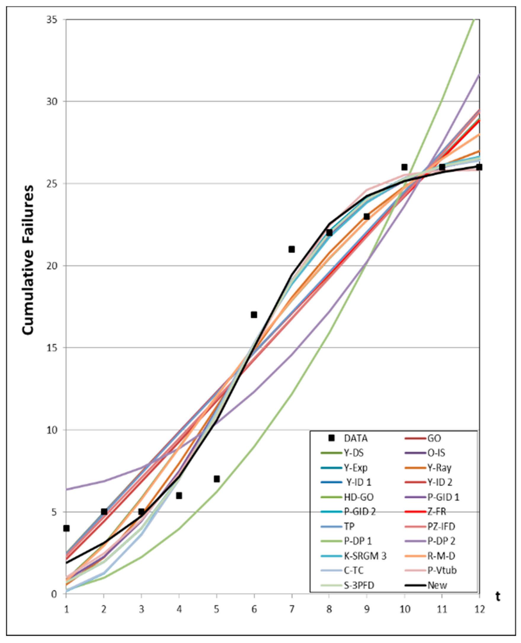
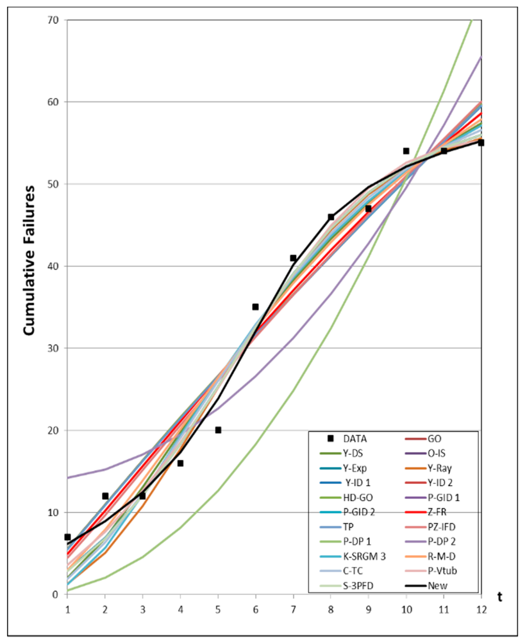
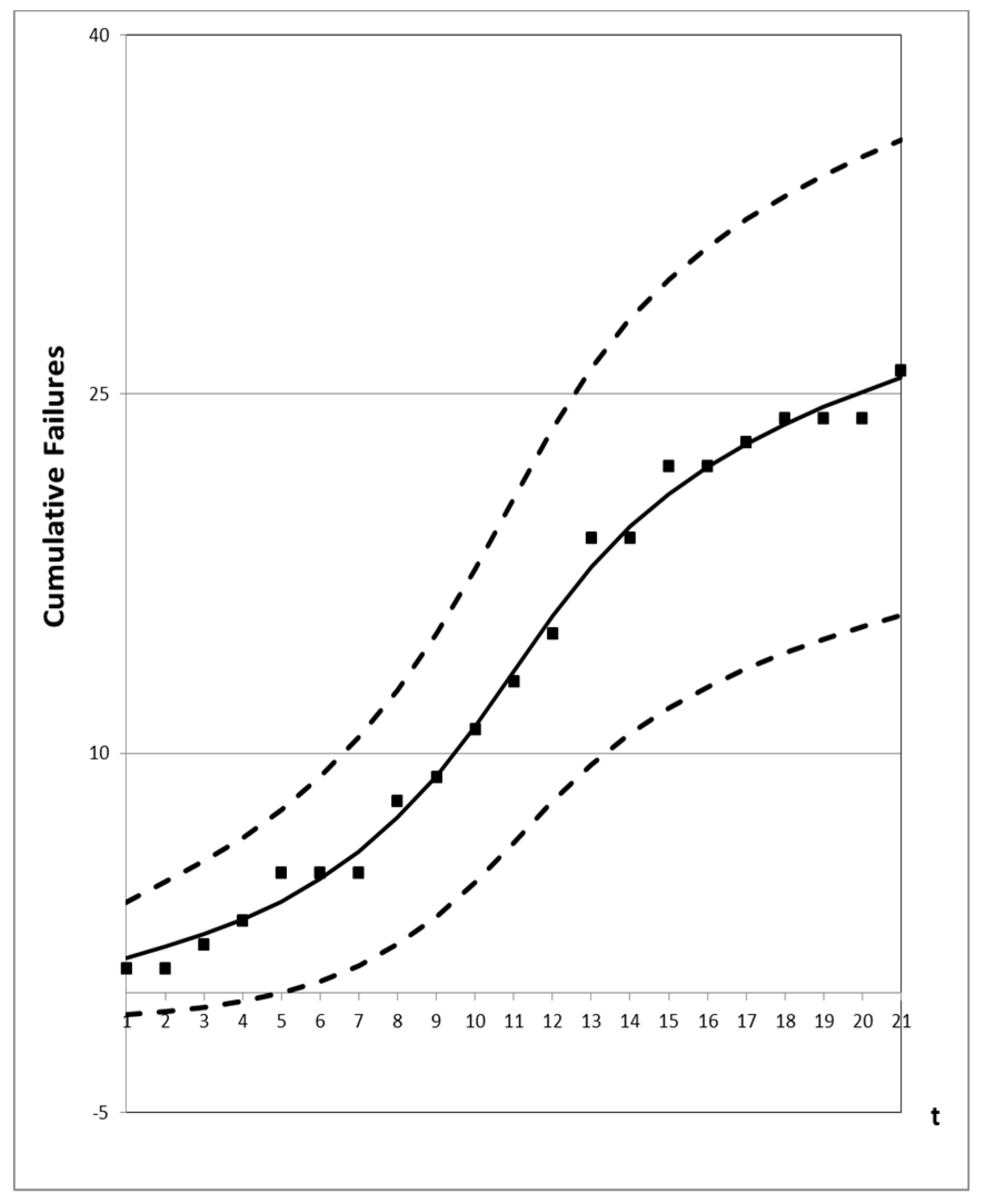
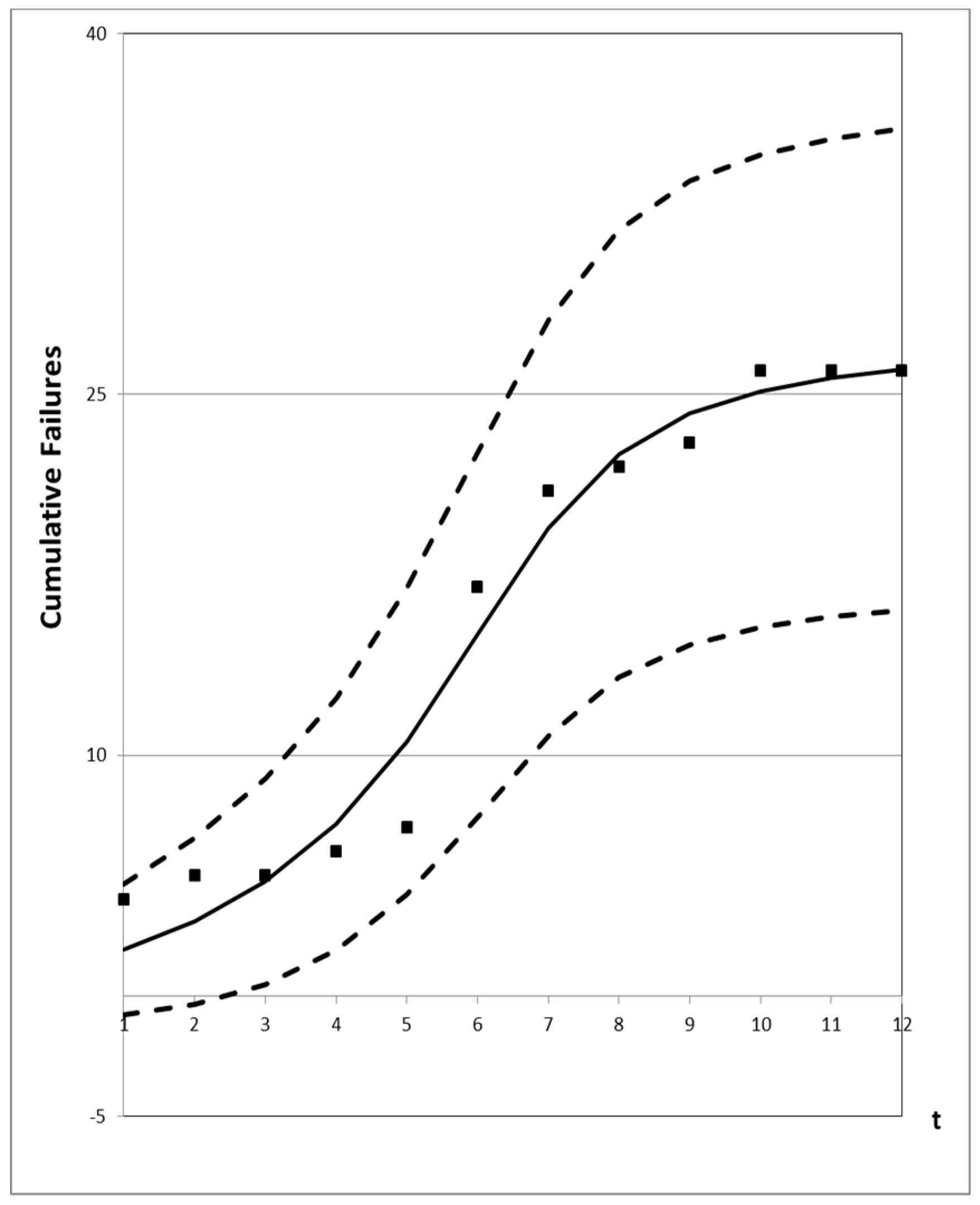
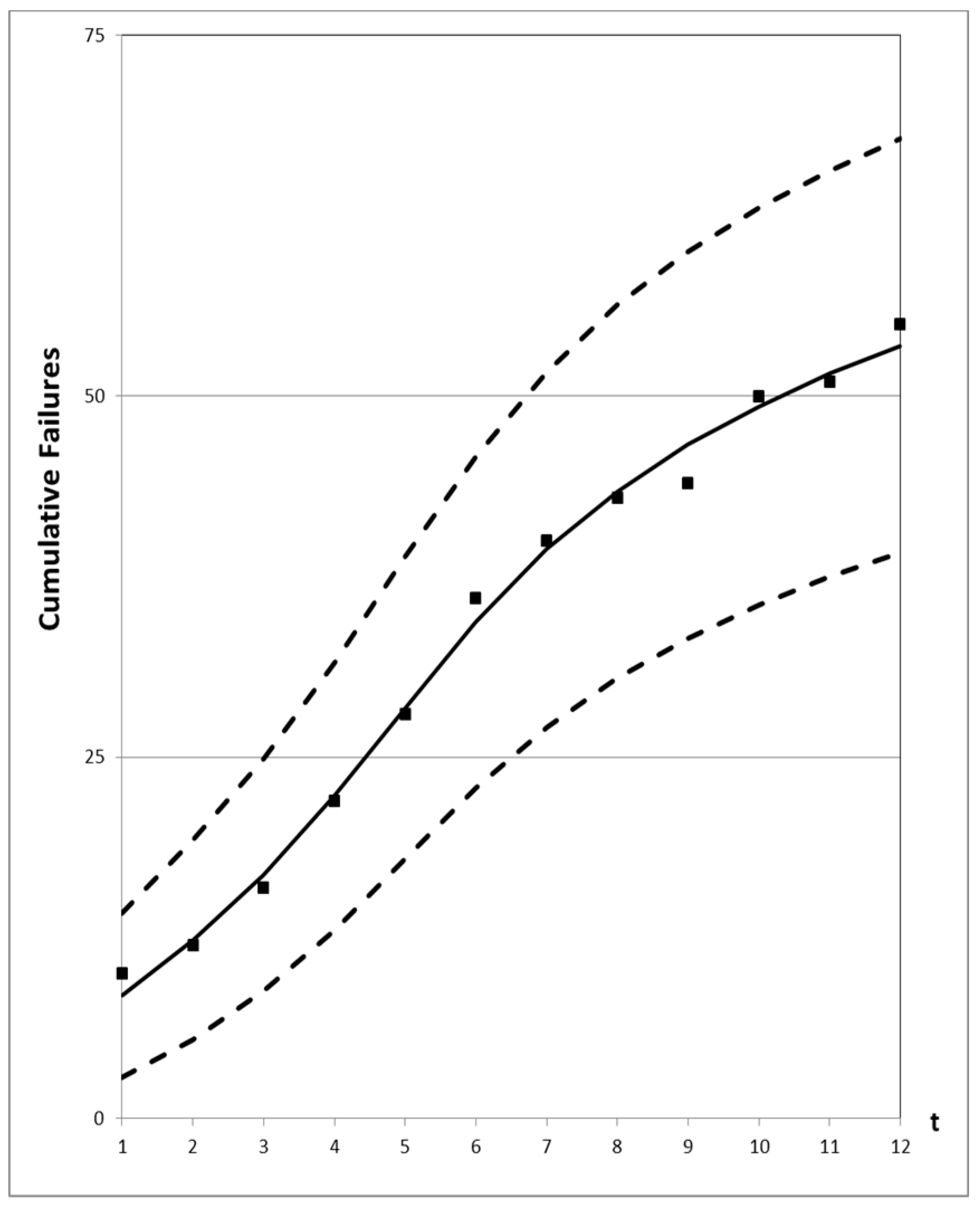
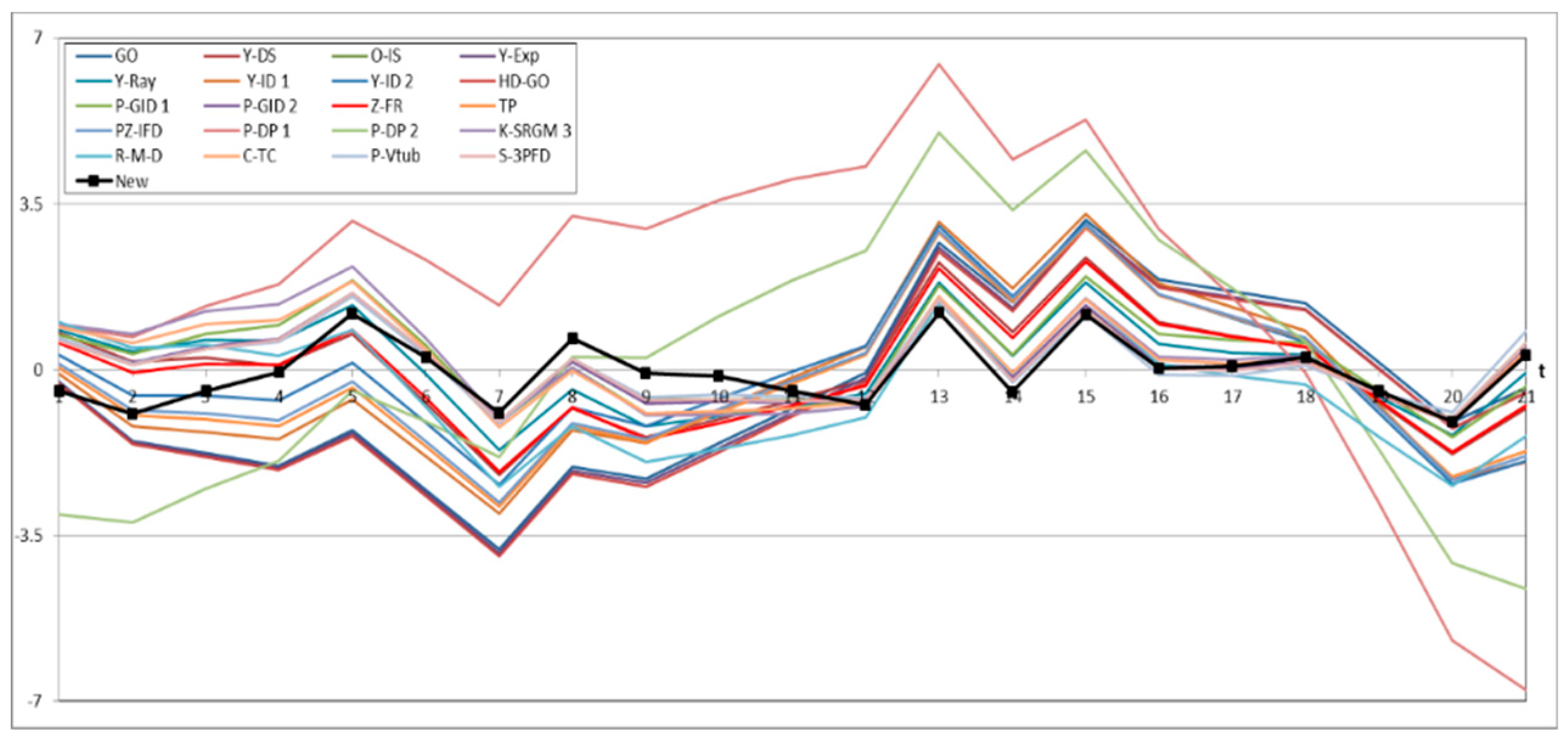
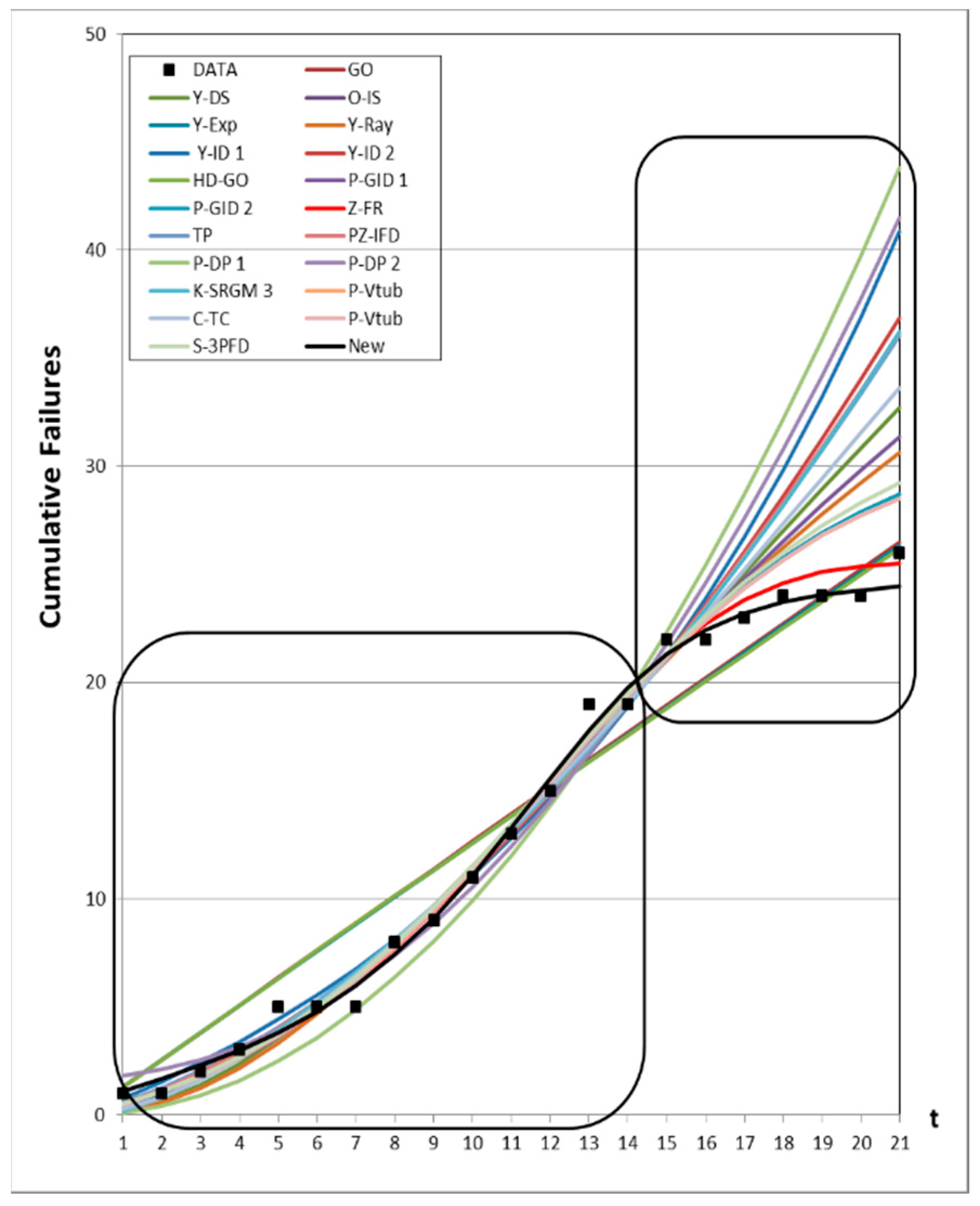
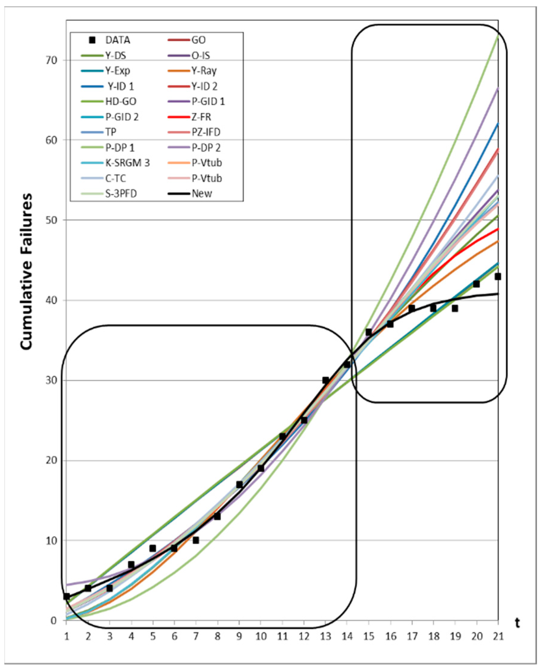
4.3. Prediction Analysis
5. Conclusions
Author Contributions
Funding
Acknowledgments
Conflicts of Interest
References
- Goel, A.L.; Okumoto, K. Time-dependent error-detection rate model for software reliability and other performance measures. IEEE Trans. Reliab. 1979, 28, 206–211. [Google Scholar] [CrossRef]
- Yamada, S.; Ohba, M.; Osaki, S. S-shaped reliability growth modeling for software fault detection. IEEE Trans. Reliab. 1983, 32, 475–484. [Google Scholar] [CrossRef]
- Ohba, M. Inflexion S-shaped software reliability growth models. In Stochastic Models in Reliability Theory; Osaki, S., Hatoyama, Y., Eds.; Springer: Berlin, Germany, 1984; pp. 144–162. [Google Scholar]
- Yamada, S.; Ohtera, H.; Narihisa, H. Software Reliability Growth Models with Testing-Effort. IEEE Trans. Reliab. 1986, 35, 19–23. [Google Scholar] [CrossRef]
- Yang, B.; Xie, M. A study of operational and testing reliability in software reliability analysis. Reliab. Eng. Syst. Saf. 2000, 70, 323–329. [Google Scholar] [CrossRef]
- Huang, C.Y.; Kuo, S.Y.; Lyu, M.R.; Lo, J.H. Quantitative software reliability modeling from testing from testing to operation. In Proceedings of the International Symposium on Software Reliability Engineering, IEEE, Los Alamitos, CA, USA, 8–11 October 2000; pp. 72–82. [Google Scholar]
- Zhang, X.; Jeske, D.; Pham, H. Calibrating software reliability models when the test environment does not match the user environment. Appl. Stoch. Models Bus. Ind. 2002, 18, 87–99. [Google Scholar] [CrossRef]
- Teng, X.; Pham, H. A new methodology for predicting software reliability in the random field environments. IEEE Trans. Reliab. 2006, 55, 458–468. [Google Scholar] [CrossRef]
- Inoue, S.; Ikeda, J.; Yamda, S. Bivariate change-point modeling for software reliability assessment with uncertainty of testing-environment factor. Ann. Oper. Res. 2016, 244, 209–220. [Google Scholar] [CrossRef]
- Li, Q.; Pham, H. A testing-coverage software reliability model considering fault removal efficiency and error generation. PLoS ONE 2017, 12, e0181524. [Google Scholar] [CrossRef] [PubMed]
- Li, Q.; Pham, H. NHPP software reliability model considering the uncertainty of operating environments with imperfect debugging and testing coverage. Appl. Math. Model. 2017, 51, 68–85. [Google Scholar] [CrossRef]
- Song, K.Y.; Chang, I.H.; Pham, H. A Three-parameter fault-detection software reliability model with the uncertainty of operating environments. J. Syst. Sci. Syst. Eng. 2017, 26, 121–132. [Google Scholar] [CrossRef]
- Song, K.Y.; Chang, I.H.; Pham, H. A software reliability model with a Weibull fault detection rate function subject to operating environments. Appl. Sci. 2017, 7, 983. [Google Scholar] [CrossRef]
- Song, K.Y.; Chang, I.H.; Pham, H. An NHPP software reliability model with S-shaped growth curve subject to random operating environments and optimal release time. Appl. Sci. 2017, 7, 1304. [Google Scholar] [CrossRef]
- Song, K.Y.; Chang, I.H.; Pham, H. Optimal Release Time and Sensitivity Analysis Using a New NHPP Software Reliability Model with Probability of Fault Removal Subject to Operating Environments. Appl. Sci. 2018, 8, 714. [Google Scholar] [CrossRef]
- Zhu, M.; Pham, H. A two-phase software reliability modeling involving with software fault dependency and imperfect fault removal. Comput. Lang. Syst. Struct. 2018, 53, 27–42. [Google Scholar] [CrossRef]
- Yamada, S.; Tokuno, K.; Osaki, S. Imperfect debugging models with fault introduction rate for software reliability assessment. Int. J. Syst. Sci. 1992, 23, 2241–2252. [Google Scholar] [CrossRef]
- Hossain, S.A.; Dahiya, R.C. Estimating the parameters of a non-homogeneous Poisson-process model for software reliability. IEEE Trans. Reliab. 1993, 42, 604–612. [Google Scholar] [CrossRef]
- Pham, H.; Nordmann, L.; Zhang, X. A general imperfect software debugging model with S-shaped fault detection rate. IEEE Trans. Reliab. 1999, 48, 169–175. [Google Scholar] [CrossRef]
- Pham, H.; Zhang, X. An NHPP software reliability models and its comparison. Int. J. Reliab. Qual. Saf. Eng. 1997, 4, 269–282. [Google Scholar] [CrossRef]
- Zhang, X.M.; Teng, X.L.; Pham, H. Considering fault removal efficiency in software reliability assessment. IEEE Trans. Syst. Man. Cybern. Part Syst. Hum. 2003, 33, 114–120. [Google Scholar] [CrossRef]
- Pham, H. System Software Reliability; Springer: London, UK, 2006. [Google Scholar]
- Pham, H. An Imperfect-debugging Fault-detection Dependent-parameter Software. Int. J. Automat. Comput. 2007, 4, 325–328. [Google Scholar] [CrossRef]
- Kapur, P.K.; Pham, H.; Anand, S.; Yadav, K. A unified approach for developing software reliability growth models in the presence of imperfect debugging and error generation. IEEE Trans. Reliab. 2011, 60, 331–340. [Google Scholar] [CrossRef]
- Roy, P.; Mahapatra, G.S.; Dey, K.N. An NHPP software reliability growth model with imperfect debugging and error generation. Int. J. Reliab. Qual. Saf. Eng. 2014, 21, 1–3. [Google Scholar] [CrossRef]
- Pham, H. A new software reliability model with Vtub-Shaped fault detection rate and the uncertainty of operating environments. Optimization 2014, 63, 1481–1490. [Google Scholar] [CrossRef]
- Chang, I.H.; Pham, H.; Lee, S.W.; Song, K.Y. A testing-coverage software reliability model with the uncertainty of operation environments. Int. J. Syst. Sci. Oper. Logist. 2014, 1, 220–227. [Google Scholar]
- Akaike, H. A new look at statistical model identification. IEEE Trans. Autom. Control 1974, 19, 716–719. [Google Scholar] [CrossRef]
- Anjum, M.; Haque, M.A.; Ahmad, N. Analysis and ranking of software reliability models based on weighted criteria value. Int. J. Inf. Technol. Comput. Sci. 2013, 2, 1–14. [Google Scholar] [CrossRef]


| No. | Model | |
|---|---|---|
| 1 | Goel–Okumoto (GO) [1] | |
| 2 | Yamada et al. (Y-DS) [2] | |
| 3 | Ohba (O-IS) [3] | |
| 4 | Yamada et al.(Y-Exp) [4] | |
| 5 | Yamata et al. (Y-Ray) [4] | |
| 6 | Yamada et al. (Y-ID 1) [17] | |
| 7 | Yamada et al. (Y-ID 2) [17] | |
| 8 | Hossain-Dahiya (HD-GO) [18] | |
| 9 | Pham et al. (P-GID 1) [19] | |
| 10 | Pham–Zhang (P-GID) [20] | |
| 11 | Zhang et al. (Z-FR) [21] | |
| 12 | Teng-Pham (TP) [8] | |
| 13 | Pham Zhang IFD (PZ-IFD) [22] | |
| 14 | Pham (DP 1) [23] | |
| 15 | Pham (DP 2) [23] | |
| 16 | Kapur et al. (SRGM-3) [24] | |
| 17 | Roy et al. (R-M-D) [25] | |
| 18 | Chang et al. (C-TC) [27] | |
| 19 | Pham (P-Vtub) [26] | |
| 20 | Song et al. (S-3PFD) [12] | |
| 21 | Proposed New Model |
| No. | Model | Parameter Estimation | MSE | RMSE | PRR | PP | AIC | R2 | Adj R2 | SAE | MAE | Variation |
|---|---|---|---|---|---|---|---|---|---|---|---|---|
| 1 | GO | = 3,923,854.7292 = 3.2 × 10⁻⁷ | 3.8672 | 1.9665 | 1.3107 | 4.7001 | 65.3539 | 0.9582 | 0.9535 | 33.7895 | 1.7784 | 2.0637 |
| 2 | Y-DS | = 39.82198 = 0.1104 | 1.4938 | 1.2222 | 12.0730 | 0.9675 | 63.9400 | 0.9838 | 0.9820 | 19.9951 | 1.0524 | 1.1926 |
| 3 | O-IS | = 26.6845,= 0.2918 = 21.6851 | 0.6745 | 0.8213 | 2.8475 | 0.6556 | 64.1770 | 0.9931 | 0.9919 | 12.9369 | 0.7187 | 0.7996 |
| 4 | Y-Exp | = 92,075.4308,= 0.3562 = 0.0005147,= 0.07514 | 4.3392 | 2.0831 | 1.3380 | 4.8827 | 69.3634 | 0.9580 | 0.9475 | 33.9888 | 1.9993 | 2.1300 |
| 5 | Y-Ray | = 29.0366,= 5.9677 = 0.000374,= 4.8158 | 1.1421 | 1.0687 | 30.3583 | 1.2435 | 67.6217 | 0.9889 | 0.9862 | 16.6930 | 0.9819 | 0.9920 |
| 6 | Y-ID 1 | = 1091.828,= 0.00098 = 0.0209 | 3.4470 | 1.8566 | 0.9414 | 2.7339 | 67.6756 | 0.9647 | 0.9584 | 30.9144 | 1.7175 | 1.8285 |
| 7 | Y-ID 2 | = 2.3351,= 0.2451 = 0.6469 | 2.5766 | 1.6052 | 0.6847 | 0.9081 | 66.5843 | 0.9736 | 0.9689 | 25.0483 | 1.3916 | 1.5265 |
| 8 | HD-GO | = 709.7827,= 0.00181 = 0.0998 | 4.1786 | 2.0442 | 1.3722 | 5.0982 | 67.3785 | 0.9572 | 0.9496 | 34.3708 | 1.9095 | 2.1867 |
| 9 | P-GID 1 | = 10.6281,= 0.37304 = 0.0817,= 17.0709 | 1.2140 | 1.1018 | 8.5407 | 1.1317 | 66.6636 | 0.9883 | 0.9853 | 17.7928 | 1.0466 | 1.0894 |
| 10 | P-GID 2 | = 7.1732,= 0.2784 = 0.2249,= 16.7796 = 19.9096 | 0.8041 | 0.8967 | 3.4790 | 0.7162 | 68.1690 | 0.9927 | 0.9902 | 13.3027 | 0.8314 | 0.8203 |
| 11 | Z-FR | = 0.5193,= 0.4377 = 5.5458,= 6.9059 = 4.6241,= 6.9172 | 1.7715 | 1.3310 | 1.8532 | 0.6332 | 70.9195 | 0.9849 | 0.9784 | 19.2629 | 1.2842 | 1.1597 |
| 12 | TP | = 6.7122,= 0.1818 = 0.0687,= 0.053 = 0.7196,= 0.1544 = 0.1534 | 3.6887 | 1.9206 | 0.7722 | 1.9488 | 74.7613 | 0.9706 | 0.9548 | 27.8156 | 1.9868 | 1.6781 |
| 13 | PZ-IFD | = 6.3355,= 0.1287 = 0.0129 | 2.8339 | 1.6834 | 0.7156 | 1.6161 | 66.8070 | 0.9710 | 0.9658 | 27.3902 | 1.5217 | 1.6445 |
| 14 | P-DP 1 | = 2.7 × 10−6 = 165.8689 | 14.5826 | 3.8187 | 172.8372 | 3.7900 | 75.9409 | 0.8423 | 0.8248 | 65.7605 | 3.4611 | 4.7568 |
| 15 | P-DP 2 | = 6879.0649,= 0.00408 = 0.3483,= 3.9986 | 9.1284 | 3.0213 | 2.1272 | 22.1461 | 78.5680 | 0.9117 | 0.8896 | 48.5622 | 2.8566 | 2.7857 |
| 16 | K-SRGM 3 | = 24.989,= 0.1385 = 0.1012,= 3.5204 | 1.2295 | 1.1088 | 768.1366 | 2.3759 | 70.3312 | 0.9881 | 0.9851 | 17.7006 | 1.0412 | 1.1036 |
| 17 | R-M-D | = 40.2018,= 0.1152 = 0.9319,= 0.1402 | 2.0059 | 1.4163 | 6379037.0905 | 1.7234 | 80.0129 | 0.9806 | 0.9757 | 22.3624 | 1.3154 | 1.5591 |
| 18 | C-TC | = 0.00432,= 2.234 = 9959.1698,= 15.2504 = 26.8334 | 1.0939 | 1.0459 | 102.3904 | 1.7481 | 70.5589 | 0.9900 | 0.9867 | 16.0422 | 1.0026 | 0.9842 |
| 19 | P-Vtub | = 1.0985,= 1.2978 = 1.5176,= 11.3848 = 25.7412 | 0.7178 | 0.8472 | 4.3863 | 0.7200 | 69.0114 | 0.9935 | 0.9913 | 12.7522 | 0.7970 | 0.7803 |
| 20 | S-3PFD | = 0.038, = 0.292 = 0.002,= 26.889 = 1488.598 | 0.7590 | 0.8712 | 2.8538 | 0.6565 | 68.1694 | 0.9931 | 0.9908 | 12.9491 | 0.8093 | 0.7980 |
| 21 | New Model | = 108,232.8195 = 1.0047,= 0.2176 = 155.5011,= 47.7965 | 0.5864 | 0.7658 | 0.5024 | 1.2025 | 66.7301 | 0.9947 | 0.9929 | 11.3783 | 0.7111 | 0.6906 |
| No. | Model | Parameter Estimation | MSE | RMSE | PRR | PP | AIC | R2 | Adj R2 | SAE | MAE | Variation |
|---|---|---|---|---|---|---|---|---|---|---|---|---|
| 1 | GO | = 5899.3694 = 0.0036 | 6.6537 | 2.5795 | 0.6859 | 1.0870 | 78.3163 | 0.9718 | 0.9687 | 43.1731 | 2.2723 | 2.6349 |
| 2 | Y-DS | = 62.3045 = 0.1185 | 3.2732 | 1.8092 | 44.3612 | 1.4298 | 81.0873 | 0.9862 | 0.9846 | 32.5216 | 1.7117 | 1.8123 |
| 3 | O-IS | = 46.5437,= 0.2409 = 12.2242 | 1.8704 | 1.3676 | 5.9546 | 0.8965 | 76.9477 | 0.9925 | 0.9912 | 21.9605 | 1.2200 | 1.3693 |
| 4 | Y-Exp | = 616.2702,= 0.1998 = 0.00048,= 36.8345 | 7.9598 | 2.8213 | 0.7015 | 1.1835 | 82.2610 | 0.9699 | 0.9623 | 44.2608 | 2.6036 | 2.7046 |
| 5 | Y-Ray | = 47.0086,= 6.2232 = 0.00029,= 6.3708 | 3.2147 | 1.7929 | 111.4178 | 1.8451 | 85.7632 | 0.9878 | 0.9848 | 27.7602 | 1.6330 | 1.8734 |
| 6 | Y-ID 1 | = 647.4658,= 0.00295 = 0.0158 | 6.2463 | 2.4993 | 0.6833 | 0.7512 | 80.9818 | 0.9750 | 0.9705 | 40.9177 | 2.2732 | 2.4195 |
| 7 | Y-ID 2 | = 68.4424,= 0.0265 = 0.0511 | 5.9996 | 2.4494 | 0.7308 | 0.6707 | 80.8924 | 0.9760 | 0.9717 | 39.9577 | 2.2199 | 2.3415 |
| 8 | HD-GO | = 709.7826,= 0.00307 = 0.7659 | 7.3398 | 2.7092 | 0.7035 | 1.2045 | 80.2859 | 0.9706 | 0.9654 | 44.4142 | 2.4675 | 2.7776 |
| 9 | P-GID 1 | = 46.4854,= 0.2410 = 0.000067,= 12.2127 | 1.9814 | 1.4076 | 5.9524 | 0.8964 | 78.9480 | 0.9925 | 0.9906 | 21.9749 | 1.2926 | 1.3673 |
| 10 | P-GID 2 | = 0.000032,= 0.2409 = 1.6139,= 12.2219 = 46.5445 | 2.1042 | 1.4506 | 5.9510 | 0.8963 | 80.9477 | 0.9925 | 0.9900 | 21.9644 | 1.3728 | 1.3683 |
| 11 | Z-FR | = 283.299,= 0.173997 = 520.118,= 0.27156 = 1.8366,= 6.9716 | 1.8601 | 1.3639 | 3.9072 | 0.7296 | 84.2304 | 0.9938 | 0.9911 | 20.1020 | 1.3401 | 1.2316 |
| 12 | TP | = 192.3412,= 0.3131 = 0.029,= 0.1954 = 1 0.0202,= 0.5938 = 0.3842 | 3.5100 | 1.8735 | 6.2127 | 0.9182 | 86.2875 | 0.9891 | 0.9832 | 28.6293 | 2.0450 | 1.6235 |
| 13 | PZ-IFD | = 13.1083,= 0.1154 = 0.0057 | 5.1126 | 2.2611 | 1.0650 | 0.6546 | 80.1375 | 0.9795 | 0.9759 | 36.4678 | 2.0260 | 2.1645 |
| 14 | P-DP 1 | = 7.6 × 10−7 = 403.0753 | 43.7600 | 6.6151 | 613.6285 | 4.5758 | 104.7474 | 0.8149 | 0.7943 | 122.0195 | 6.4221 | 8.8176 |
| 15 | P-DP 2 | = 3343.5848,= 0.00728 = 0.3771,= 7.7754 | 21.3006 | 4.6153 | 1.4148 | 5.4631 | 96.7740 | 0.9194 | 0.8992 | 76.4876 | 4.4993 | 4.2597 |
| 16 | K-SRGM 3 | = 21.2662,= 0.3874 = 0.6255,= 0.8962 | 3.9525 | 1.9881 | 439.7196 | 2.0575 | 90.5520 | 0.9850 | 0.9813 | 32.8146 | 1.9303 | 1.9720 |
| 17 | R-M-D | = 157.3012,= 0.0144 = 1.2327,= 0.3454 | 4.6378 | 2.1536 | 6.7102 | 0.9139 | 83.3777 | 0.9824 | 0.9781 | 34.4805 | 2.0283 | 2.0045 |
| 18 | C-TC | = 0.00607,= 1.864 = 9445.7865,= 93.4027 = 48.9629 | 3.3003 | 1.8167 | 57.3169 | 1.5788 | 86.4442 | 0.9882 | 0.9843 | 28.8335 | 1.8021 | 1.7301 |
| 19 | P-Vtub | = 1.2575,= 0.98699 = 1.4559,= 16.4583 = 45.2916 | 1.9851 | 1.4089 | 4.7454 | 0.8092 | 80.7744 | 0.9929 | 0.9906 | 21.7860 | 1.3616 | 1.3047 |
| 20 | S-3PFD | = 3.078,= 0.2410 = 0.170,= 46.8430 = 999.493 | 2.1046 | 1.4507 | 5.9567 | 0.8967 | 80.9477 | 0.9925 | 0.9900 | 21.9661 | 1.3729 | 1.3680 |
| 21 | New Model | = 9198.8054 = 0.7274,= 0.2584 = 5.9777,= 50.2841 | 0.8470 | 0.9203 | 0.1159 | 0.1355 | 77.0423 | 0.9970 | 0.9960 | 14.0367 | 0.8773 | 0.8232 |
| No. | Model | Parameter Estimation | MSE | RMSE | PRR | PP | AIC | R2 | Adj R2 | SAE | MAE | Variation |
|---|---|---|---|---|---|---|---|---|---|---|---|---|
| 1 | GO | = 464.5247 = 0.00536 | 9.0920 | 3.0153 | 0.9284 | 1.4443 | 62.4128 | 0.9069 | 0.8862 | 28.2200 | 2.8220 | 2.8899 |
| 2 | Y-DS | = 35.8316 = 0.2396 | 7.0034 | 2.6464 | 13.4415 | 1.6025 | 63.3503 | 0.9283 | 0.9124 | 24.4671 | 2.4467 | 2.5391 |
| 3 | O-IS | = 26.9254,= 0.6204 = 30.0163 | 5.1138 | 2.2614 | 22.9009 | 1.4436 | 57.8013 | 0.9529 | 0.9352 | 18.2801 | 2.0311 | 2.1767 |
| 4 | Y-Exp | = 6456.5057,= 0.1461 = 0.00495,= 0.5332 | 11.3652 | 3.3712 | 0.9284 | 1.4442 | 66.4149 | 0.9069 | 0.8537 | 28.2211 | 3.5276 | 2.8900 |
| 5 | Y-Ray | = 28.4774,= 23.884 = 2.3 × 10⁻⁶,= 746.3198 | 7.4818 | 2.7353 | 36.8584 | 1.5855 | 66.0682 | 0.9387 | 0.9037 | 21.3831 | 2.6729 | 2.5201 |
| 6 | Y-ID 1 | = 316.6384,= 0.00789 = 0.0016 | 10.1040 | 3.1787 | 0.9243 | 1.4515 | 64.3742 | 0.9069 | 0.8720 | 28.1806 | 3.1312 | 2.8893 |
| 7 | Y-ID 2 | = 4.4246,= 0.4623 = 0.5756 | 9.9746 | 3.1583 | 1.2645 | 1.2271 | 64.9967 | 0.9081 | 0.8736 | 29.0765 | 3.2307 | 2.8578 |
| 8 | HD-GO | = 446.4583,= 0.00558 = 1 × 10⁻⁹ | 10.1022 | 3.1784 | 0.9279 | 1.4447 | 64.4008 | 0.9069 | 0.8720 | 28.2149 | 3.1350 | 2.8889 |
| 9 | P-GID 1 | = 27.1316,= 0.5709 = 2.1 × 10⁻¹¹,= 22.163 | 5.8233 | 2.4132 | 14.4703 | 1.3672 | 59.5427 | 0.9523 | 0.9250 | 18.2613 | 2.2827 | 2.1505 |
| 10 | P-GID 2 | = 1 × 10⁻¹⁰,= 0.6204 = 0.0387,= 30.0163 = 26.9254 | 6.5749 | 2.5642 | 22.9009 | 1.4436 | 61.8013 | 0.9529 | 0.9136 | 18.2801 | 2.6114 | 2.1767 |
| 11 | Z-FR | = 46.9742,= 0.1457 = 0.1382,= 0.1987 = 0.0596,= 0.4732 | 14.9849 | 3.8710 | 0.9416 | 1.4419 | 70.2105 | 0.9079 | 0.7975 | 28.0342 | 4.6724 | 2.8709 |
| 12 | TP | = 107.787,= 2.6× 10−8 = 0.2044,= 1.1 × 10−7 = 1.1232,= 0.00142 = 0.000061 | 18.2859 | 4.2762 | 0.9453 | 1.4258 | 72.7010 | 0.9064 | 0.7426 | 28.3832 | 5.6766 | 2.9222 |
| 13 | PZ-IFD | = 281.2703,= 0.0083 = 0.000031 | 10.2029 | 3.1942 | 1.0336 | 1.2844 | 64.9647 | 0.9060 | 0.8707 | 29.1055 | 3.2339 | 2.8893 |
| 14 | P-DP 1 | = 2.0 × 10−6 = 1115.343 | 34.4416 | 5.8687 | 246.9020 | 2.6126 | 86.7862 | 0.6474 | 0.5690 | 54.1442 | 5.4144 | 6.8563 |
| 15 | P-DP 2 | = 2070.3183,= 0.0125 = 8.7785,= 19.516 | 21.2667 | 4.6116 | 1.0306 | 1.5407 | 72.4094 | 0.8258 | 0.7263 | 41.3919 | 5.1740 | 3.9346 |
| 16 | K-SRGM 3 | = 27.2536,= 0.1691 = 0.00,= 9.476 | 7.2970 | 2.7013 | 444.6336 | 1.9569 | 71.8813 | 0.9402 | 0.9061 | 20.6929 | 2.5866 | 2.5289 |
| 17 | R-M-D | = 35.969,= 0.24269 = 0.9901,= 0.2427 | 8.7525 | 2.9585 | 15.6161 | 1.6246 | 67.6920 | 0.9283 | 0.8873 | 24.4048 | 3.0506 | 2.5408 |
| 18 | C-TC | = 0.2739,= 2.604 = 12.2099,= 50.5848 = 26.7229 | 7.9859 | 2.8259 | 302.4876 | 1.9056 | 71.5591 | 0.9428 | 0.8951 | 19.7573 | 2.8225 | 2.4696 |
| 19 | P-Vtub | = 1.9764,= 0.8427 = 33.7789,= 804.4101 = 25.8336 | 6.1408 | 2.4781 | 9.4191 | 1.1932 | 59.4576 | 0.9560 | 0.9193 | 18.0194 | 2.5742 | 2.0513 |
| 20 | S-3PFD | = 10.6227,= 0.6211 = 1.3819,= 27.808 = 397.0025 | 6.6075 | 2.5705 | 23.0454 | 1.4412 | 61.9886 | 0.9526 | 0.9132 | 18.3461 | 2.6209 | 2.1986 |
| 21 | New Model | = 9643.4774 = 1.3046,= 0.3131 = 1.4073,= 27.70003 | 4.4412 | 2.1074 | 1.7190 | 0.7376 | 54.3482 | 0.9682 | 0.9416 | 15.4691 | 2.2099 | 1.7189 |
| No. | Model | Parameter Estimation | MSE | RMSE | PRR | PP | AIC | R2 | Adj R2 | SAE | MAE | Variation |
|---|---|---|---|---|---|---|---|---|---|---|---|---|
| 1 | GO | = 270.1056 = 0.02075 | 18.3634 | 4.2853 | 0.3249 | 0.4503 | 80.3676 | 0.9519 | 0.9412 | 41.4895 | 4.1490 | 4.1060 |
| 2 | Y-DS | = 69.8210 = 0.2627 | 14.0418 | 3.7472 | 6.7145 | 0.8711 | 82.3170 | 0.9632 | 0.9550 | 35.4185 | 3.5418 | 3.6596 |
| 3 | O-IS | = 59.0235,= 0.4417 = 9.7336 | 10.8677 | 3.2966 | 2.6138 | 0.6298 | 75.1254 | 0.9744 | 0.9647 | 28.1022 | 3.1225 | 3.0973 |
| 4 | Y-Exp | = 5981.4323,= 0.0778 = 0.0199,= 0.6051 | 22.9599 | 4.7916 | 0.3250 | 0.4498 | 84.3686 | 0.9518 | 0.9243 | 41.5089 | 5.1886 | 4.1045 |
| 5 | Y-Ray | = 57.701,= 58.8436 = 2.6 × 10⁻⁸,= 30,017.6386 | 16.6108 | 4.0756 | 20.8256 | 1.0967 | 86.7089 | 0.9652 | 0.9453 | 31.4668 | 3.9334 | 3.9710 |
| 6 | Y-ID 1 | = 270.1054,= 0.02075 = 1.4 × 10⁻⁸ | 20.4038 | 4.5171 | 0.3249 | 0.4503 | 82.3676 | 0.9519 | 0.9338 | 41.4896 | 4.6100 | 4.1060 |
| 7 | Y-ID 2 | = 270.1041,= 0.0208 = 9.9 × 10⁻⁸ | 20.4110 | 4.5179 | 0.3238 | 0.4546 | 82.3842 | 0.9518 | 0.9338 | 41.3885 | 4.5987 | 4.1220 |
| 8 | HD-GO | = 270.1056,= 0.0208 = 1 × 10⁻⁹ | 20.4111 | 4.5179 | 0.3238 | 0.4546 | 82.3843 | 0.9518 | 0.9338 | 41.3882 | 4.5987 | 4.1221 |
| 9 | P-GID 1 | = 59.0239,= 0.4417 = 1.4 × 10⁻¹⁰,= 9.7338 | 12.2261 | 3.4966 | 2.6139 | 0.6298 | 77.1255 | 0.9744 | 0.9597 | 28.1025 | 3.5128 | 3.0972 |
| 10 | P-GID 2 | = 1 × 10⁻¹⁰,= 0.4418 = 0.1819,= 9.7336 = 59.0235 | 13.9727 | 3.7380 | 2.6113 | 0.6298 | 79.1245 | 0.9744 | 0.9530 | 28.0991 | 4.0142 | 3.0944 |
| 11 | Z-FR | = 88.285,= 0.2295 = 1.1342,= 0.1063 = 0.1169,= 1.0616 | 25.7905 | 5.0784 | 0.4037 | 0.4399 | 85.8969 | 0.9594 | 0.9107 | 38.1771 | 6.3629 | 3.7579 |
| 12 | TP | = 5.5526,= 0.1157 = 2.7637,= 0.2783 = 0.1523,= 0.0844 = 0.0632 | 36.2811 | 6.0234 | 0.3289 | 0.4475 | 90.2214 | 0.9524 | 0.8692 | 41.3061 | 8.2612 | 4.0814 |
| 13 | PZ-IFD | = 13.351,= 0.3015 = 1 × 10⁻¹⁰ | 18.9582 | 4.3541 | 0.5563 | 0.4514 | 82.7552 | 0.9553 | 0.9385 | 41.5660 | 4.6184 | 3.9404 |
| 14 | P-DP 1 | = 5.5 × 10−8 = 3036.6077 | 146.2340 | 12.0927 | 193.5342 | 2.9279 | 132.5762 | 0.6166 | 0.5314 | 120.1415 | 12.0141 | 15.5642 |
| 15 | P-DP 2 | = 71,469.8104,= 0.00313 = 8.7 × 10⁻⁶,= 13.8578 | 64.8252 | 8.0514 | 0.7452 | 1.5864 | 108.7149 | 0.8640 | 0.7863 | 71.5589 | 8.9449 | 6.8673 |
| 16 | K-SRGM3 | = 47.998,= 0.9041 = 0.2937,= 0.394 | 18.9589 | 4.3542 | 23.2982 | 1.1112 | 91.8189 | 0.9602 | 0.9375 | 34.9075 | 4.3634 | 3.8929 |
| 17 | R-M-D | = 66.7919,= 0.2313 = 1.10797,= 0.23129 | 16.9597 | 4.1182 | 2.1336 | 0.6528 | 83.0580 | 0.9644 | 0.9441 | 35.9526 | 4.4941 | 3.5372 |
| 18 | C-TC | = 0.3805,= 1.7675 = 6021.5496 = 33,686.7619,= 61.0142 | 18.1240 | 4.2572 | 7.6284 | 0.8839 | 86.1250 | 0.9667 | 0.9390 | 32.2656 | 4.6094 | 3.5264 |
| 19 | P-Vtub | = 2.3187,= 0.6928 = 13.81799,= 269.3212 = 55.7854 | 12.2331 | 3.4976 | 1.2508 | 0.4708 | 76.2949 | 0.9775 | 0.9588 | 26.5196 | 3.7885 | 2.8320 |
| 20 | S-3PFD | = 223.3416,= 0.4424 = 4.4956,= 59.245 = 1213.0757 | 13.9742 | 3.7382 | 2.6264 | 0.6308 | 79.1281 | 0.9744 | 0.9530 | 28.0662 | 4.0095 | 3.0997 |
| 21 | New Model | = 42763.1241 = 1.6385,= 0.2005 = 12.6879,= 65.868 | 6.7120 | 2.5908 | 0.1812 | 0.1363 | 70.5195 | 0.9877 | 0.9774 | 18.2230 | 2.6033 | 2.0735 |
| No. | Model | Parameter Estimation | MSE | RMSE | PRR | PP | AIC | R2 | Adj R2 | SAE | MAE | Variation |
|---|---|---|---|---|---|---|---|---|---|---|---|---|
| 1 | GO | = 94.3479 = 0.0733 | 4.0245 | 2.0061 | 0.2932 | 0.1627 | 57.7077 | 0.9855 | 0.9822 | 19.4198 | 1.9420 | 1.9150 |
| 2 | Y-DS | = 57.5047 = 0.3437 | 8.2095 | 2.8652 | 7.3903 | 0.6184 | 69.6185 | 0.9704 | 0.9638 | 20.9577 | 2.0958 | 3.0188 |
| 3 | O-IS | = 65.8343,= 0.2055 = 1.2874 | 4.0555 | 2.0138 | 0.4802 | 0.1903 | 60.1404 | 0.9868 | 0.9819 | 17.0533 | 1.8948 | 1.8479 |
| 4 | Y-Exp | = 3344.357,= 0.1819 = 0.0718,= 0.1584 | 5.0365 | 2.2442 | 0.2929 | 0.1625 | 61.7078 | 0.9855 | 0.9771 | 19.4216 | 2.4277 | 1.9171 |
| 5 | Y-Ray | = 62.3356,= 0.038 = 0.0315,= 51.9474 | 15.0669 | 3.8816 | 18.8397 | 0.8508 | 81.3798 | 0.9565 | 0.9316 | 26.5145 | 3.3143 | 3.7589 |
| 6 | Y-ID 1 | = 94.3479,= 0.0733 = 1.1 × 10⁻⁹ | 4.4716 | 2.1146 | 0.2932 | 0.1627 | 59.7077 | 0.9855 | 0.9800 | 19.4198 | 2.1578 | 1.9150 |
| 7 | Y-ID 2 | = 94.3479,= 0.0733 = 1 × 10⁻¹⁰ | 4.4716 | 2.1146 | 0.2932 | 0.1627 | 59.7077 | 0.9855 | 0.9800 | 19.4198 | 2.1578 | 1.9150 |
| 8 | HD-GO | = 94.3479,= 0.0733 = 0.000109 | 4.4716 | 2.1146 | 0.2932 | 0.1627 | 59.7077 | 0.9855 | 0.9800 | 19.4198 | 2.1578 | 1.9150 |
| 9 | P-GID 1 | = 65.8343,= 0.2055 = 3.8 × 10⁻⁸,= 1.2874 | 4.5624 | 2.1360 | 0.4802 | 0.1903 | 62.1404 | 0.9868 | 0.9793 | 17.0533 | 2.1317 | 1.8479 |
| 10 | P-GID 2 | = 0.0023,= 0.2055 = 0.2328,= 1.2874 = 65.832 | 5.2142 | 2.2835 | 0.4803 | 0.1903 | 64.1404 | 0.9868 | 0.9759 | 17.0539 | 2.4363 | 1.8480 |
| 11 | Z-FR | = 27.83996,= 0.1217 = 5.0642,= 0.2853 = 1.3182,= 0.7382 | 6.0591 | 2.4615 | 0.4518 | 0.1844 | 66.1861 | 0.9869 | 0.9711 | 17.0776 | 2.8463 | 1.8421 |
| 12 | TP | = 14.3726,= 0.1574 = 10.3379,= 2.9351 = 0.1765,= 0.2112 = 0.05296 | 7.8879 | 2.8085 | 0.3120 | 0.1652 | 67.7199 | 0.9858 | 0.9609 | 18.9981 | 3.7996 | 1.8967 |
| 13 | PZ-IFD | = 6.4775,= 0.6673 = 1 × 10⁻¹⁰ | 9.0608 | 3.0101 | 0.8594 | 0.2657 | 62.8008 | 0.9706 | 0.9595 | 25.3217 | 2.8135 | 2.9951 |
| 14 | P-DP 1 | = 0.0115 = 6.5411 | 183.4378 | 13.5439 | 432.0333 | 3.4669 | 124.8012 | 0.3380 | 0.1909 | 136.0472 | 13.6047 | 18.4397 |
| 15 | P-DP 2 | = 36,611.3949,= 0.004045 = 15.3658,= 90.9356 | 43.7504 | 6.6144 | 0.5473 | 1.0956 | 81.2894 | 0.8737 | 0.8015 | 57.2136 | 7.1517 | 5.6431 |
| 16 | K-SRGM3 | = 55.9248,= 5.8366 = 0.2215,= 0.029 | 6.6314 | 2.5751 | 1.9490 | 0.3686 | 66.8324 | 0.9809 | 0.9699 | 19.5164 | 2.4396 | 2.3443 |
| 17 | R-M-D | = 39.8594,= 0.18996 = 1.7852,= 0.1900 | 4.6755 | 2.1623 | 0.4548 | 0.1884 | 62.0841 | 0.9865 | 0.9788 | 17.5748 | 2.1969 | 1.8633 |
| 18 | C-TC | = 0.1375,= 1.0738 = 16,035.1043 = 24,002.2196,= 80.5179 | 5.6419 | 2.3753 | 0.4285 | 0.1883 | 64.2419 | 0.9857 | 0.9739 | 18.3880 | 2.6269 | 1.9083 |
| 19 | P-Vtub | = 2.3789,= 0.6047 = 1.2364,= 14.6987 = 64.9314 | 4.4144 | 2.1010 | 0.2444 | 0.1304 | 62.5181 | 0.9888 | 0.9796 | 16.5855 | 2.3694 | 1.6903 |
| 20 | S-3PFD | = 0.05496,= 0.2072 = 0.0245,= 68.5181 = 25.0097 | 5.2143 | 2.2835 | 0.4812 | 0.1905 | 64.1366 | 0.9868 | 0.9759 | 17.0484 | 2.4355 | 1.8470 |
| 21 | New Model | = 276.2278 = 1.1084,= 0.2693 = 54.0622,= 93.8052 | 2.3671 | 1.5385 | 0.0412 | 0.0333 | 58.7819 | 0.9940 | 0.9890 | 11.4867 | 1.6410 | 1.2284 |
| No. | Model | Parameter Estimation | MSE | RMSE | PRR | PP | AIC | R2 | Adj R2 | SAE | MAE | Variation | PreSSE |
|---|---|---|---|---|---|---|---|---|---|---|---|---|---|
| 1 | GO | = 2439.1963 = 0.00052 | 4.8579 | 2.2041 | 1.3269 | 4.8721 | 53.2386 | 0.9199 | 0.9076 | 29.4319 | 2.1023 | 2.5172 | 5.7456 |
| 2 | Y-DS | = 81.5159 = 0.0657 | 0.8455 | 0.9195 | 25.1885 | 1.1392 | 52.1261 | 0.9861 | 0.9839 | 11.1007 | 0.7929 | 0.9257 | 128.7087 |
| 3 | O-IS | = 32.2358,= 0.2378 = 16.9353 | 0.6685 | 0.8176 | 1.4552 | 0.4588 | 52.1602 | 0.9898 | 0.9872 | 9.4132 | 0.7241 | 0.7726 | 36.1311 |
| 4 | Y-Exp | = 8326.9505,= 0.5383 = 0.00029,= 0.9697 | 5.6573 | 2.3785 | 1.3088 | 4.7500 | 57.2550 | 0.9201 | 0.8910 | 29.2644 | 2.4387 | 2.4581 | 6.0419 |
| 5 | Y-Ray | = 54.2003,= 0.0486 = 0.00296,= 35.7066 | 1.0206 | 1.0102 | 39.9442 | 1.3655 | 56.1363 | 0.9856 | 0.9803 | 11.9100 | 0.9925 | 0.9885 | 70.2926 |
| 6 | Y-ID 1 | = 174.82114,= 0.00407 = 0.08606 | 1.0997 | 1.0487 | 0.4140 | 0.6004 | 53.9407 | 0.9832 | 0.9790 | 10.7461 | 0.8266 | 0.9927 | 518.5369 |
| 7 | Y-ID 2 | = 26.9978,= 0.0173 = 0.3124 | 0.8788 | 0.9374 | 0.9227 | 0.4135 | 53.3683 | 0.9865 | 0.9832 | 8.7974 | 0.6767 | 0.8735 | 299.6604 |
| 8 | HD-GO | = 709.7826,= 0.00179 = 27.17296 | 5.3433 | 2.3116 | 1.3283 | 4.8597 | 55.3403 | 0.9182 | 0.8978 | 29.6288 | 2.2791 | 2.4842 | 6.2455 |
| 9 | P-GID 1 | = 12.7655,= 0.2324 = 0.095,= 6.7409 | 0.7999 | 0.8944 | 1.9120 | 0.5175 | 54.5868 | 0.9887 | 0.9846 | 9.6560 | 0.8047 | 0.8168 | 89.6441 |
| 10 | P-GID 2 | = 0.00079,= 0.2378 = 6.79798,= 16.9353 = 32.235 | 0.7900 | 0.8888 | 1.4552 | 0.4588 | 56.1602 | 0.9898 | 0.9847 | 9.4132 | 0.8557 | 0.7726 | 36.1309 |
| 11 | Z-FR | = 339.2109,= 0.2114 = 208.6339,= 0.1286 = 0.2734,= 13.3842 | 0.7917 | 0.8897 | 1.3398 | 0.4410 | 57.6773 | 0.9907 | 0.9845 | 9.2198 | 0.9220 | 0.7383 | 4.4041 |
| 12 | TP | = 1.9773,= 0.2819 = 0.6614,= 0.2226 = 2.2607,= 0.0576 = 0.0702 | 1.2346 | 1.1111 | 0.7866 | 0.4119 | 61.1905 | 0.9869 | 0.9755 | 8.9309 | 0.9923 | 0.8616 | 258.9145 |
| 13 | PZ-IFD | = 3.0369,= 0.1407 = 0.1038 | 0.8589 | 0.9268 | 1.1519 | 0.4317 | 53.2961 | 0.9869 | 0.9836 | 8.8436 | 0.6803 | 0.8636 | 268.2888 |
| 14 | P-DP 1 | = 0.00053 = 13.6882 | 2.5693 | 1.6029 | 89.2144 | 2.1491 | 55.2758 | 0.9577 | 0.9511 | 19.9041 | 1.4217 | 2.0091 | 803.4099 |
| 15 | P-DP 2 | = 16,554.0442,= 0.00323 = 1.1159,= 1.8408 | 1.4601 | 1.2083 | 0.6654 | 2.0357 | 56.3830 | 0.9794 | 0.9719 | 12.3365 | 1.0280 | 1.0812 | 598.1091 |
| 16 | K-SRGM 3 | = 43.9312,= 1.3062 = 2.2423,= 0.0265 | 1.0199 | 1.0099 | 20.5291 | 0.9348 | 56.6049 | 0.9856 | 0.9804 | 10.1636 | 0.8470 | 0.9148 | 264.3312 |
| 17 | R-M-D | = 153.5748,= 0.0327 = 1.0556,= 0.0463 | 0.9091 | 0.9535 | 2.6861 | 0.5630 | 55.2528 | 0.9872 | 0.9825 | 9.2852 | 0.7738 | 0.8606 | 188.6321 |
| 18 | C-TC | = 0.0288,= 1.6825 = 193.5851,= 167.6135 = 86.0872 | 1.0215 | 1.0107 | 8.9612 | 0.8232 | 57.6870 | 0.9868 | 0.9802 | 10.0127 | 0.9102 | 0.8859 | 160.1096 |
| 19 | P-Vtub | = 1.2816,= 0.9844 = 1.1473,= 20.7523 = 31.4297 | 0.7830 | 0.8849 | 1.3879 | 0.4508 | 56.1136 | 0.9899 | 0.9848 | 9.3983 | 0.8544 | 0.7681 | 32.5458 |
| 20 | S-3PFD | = 0.1496,= 0.2372 = 0.1982,= 36.9478 = 62.4407 | 0.8172 | 0.9040 | 1.3089 | 0.4455 | 56.1928 | 0.9894 | 0.9841 | 9.7423 | 0.8857 | 0.7774 | 45.9267 |
| 21 | New Model | = 10453.17249 = 0.53348,= 0.4174 = 0.1175,= 24.9924 | 0.5915 | 0.7691 | 0.3380 | 0.6053 | 54.8572 | 0.9923 | 0.9885 | 8.2769 | 0.7524 | 0.6591 | 2.6780 |
| No. | Model | Parameter Estimation | MSE | RMSE | PRR | PP | AIC | R2 | Adj R2 | SAE | MAE | Variation | PreSSE |
|---|---|---|---|---|---|---|---|---|---|---|---|---|---|
| 1 | GO | = 3631.5077 = 0.00058856 | 8.0914 | 2.8445 | 0.6812 | 1.1134 | 61.1966 | 0.9463 | 0.9380 | 36.5962 | 2.6140 | 3.0456 | 13.3815 |
| 2 | Y-DS | = 92.9084 = 0.08688 | 2.7180 | 1.6486 | 70.6100 | 1.6218 | 65.0441 | 0.9820 | 0.9792 | 19.8586 | 1.4185 | 1.8435 | 157.7642 |
| 3 | O-IS | = 76.8382,= 0.1513 = 9.348 | 1.5104 | 1.2290 | 2.7478 | 0.6084 | 61.0251 | 0.9907 | 0.9884 | 15.2338 | 1.1718 | 1.1949 | 276.1112 |
| 4 | Y-Exp | = 16,029.2962,= 0.2561 = 0.000375,= 1.3887 | 9.4224 | 3.0696 | 0.6816 | 1.1158 | 65.1857 | 0.9464 | 0.9269 | 36.5870 | 3.0489 | 3.0523 | 13.4557 |
| 5 | Y-Ray | = 83.3575,= 0.06002 = 0.005,= 20.2075 | 3.7509 | 1.9367 | 122.7334 | 1.9015 | 70.1373 | 0.9787 | 0.9709 | 20.9782 | 1.7482 | 2.1406 | 64.8807 |
| 6 | Y-ID 1 | = 1829.4685,= 0.00074 = 0.0672 | 1.7208 | 1.3118 | 1.5540 | 0.4759 | 61.5783 | 0.9894 | 0.9867 | 16.5054 | 1.2696 | 1.2638 | 826.9275 |
| 7 | Y-ID 2 | = 2404.9698,= 0.00049 = 0.1324 | 1.6375 | 1.2796 | 2.2863 | 0.5616 | 61.5103 | 0.9899 | 0.9874 | 15.9021 | 1.2232 | 1.2062 | 605.1401 |
| 8 | HD-GO | = 709.7827,= 0.00306 = 1× 10⁻⁹ | 9.1979 | 3.0328 | 0.6912 | 1.1752 | 63.4061 | 0.9433 | 0.9292 | 37.7317 | 2.9024 | 3.1490 | 12.6426 |
| 9 | P-GID 1 | = 45.3264,= 0.1489 = 0.0343,= 5.1894 | 1.6792 | 1.2958 | 2.9736 | 0.6315 | 63.1427 | 0.9904 | 0.9870 | 15.3907 | 1.2826 | 1.2188 | 306.8552 |
| 10 | P-GID 2 | = 0.00085,= 0.1513 = 0.8954,= 9.34796 = 76.8381 | 1.7850 | 1.3360 | 2.7477 | 0.6084 | 65.0251 | 0.9907 | 0.9860 | 15.2335 | 1.3849 | 1.1948 | 276.1485 |
| 11 | Z-FR | = 110.9274,= 0.1443 = 243.7368,= 0.04498 = 2.4367,= 2.1721 | 1.8974 | 1.3774 | 2.9162 | 0.6253 | 66.7569 | 0.9910 | 0.9850 | 14.8415 | 1.4841 | 1.1887 | 129.7523 |
| 12 | TP | = 3.1572,= 0.1481 = 5.3435,= 0.1162 = 18.143,= 0.0997 = 0.0547 | 2.1636 | 1.4709 | 2.7535 | 0.6092 | 68.9644 | 0.9908 | 0.9827 | 15.1312 | 1.6812 | 1.1850 | 244.6593 |
| 13 | PZ-IFD | = 31.2103,= 0.038 = 0.0429 | 1.6279 | 1.2759 | 2.2668 | 0.5577 | 61.4700 | 0.9900 | 0.9875 | 15.9819 | 1.2294 | 1.2277 | 583.1510 |
| 14 | P-DP 1 | = 0.00055 = 17.3503 | 10.7490 | 3.2786 | 328.0224 | 2.9526 | 72.2485 | 0.9287 | 0.9177 | 44.4948 | 3.1782 | 4.6393 | 2211.9360 |
| 15 | P-DP 2 | = 59,270.7316,= 0.00215 = 6.7491,= 10.6115 | 2.4626 | 1.5693 | 0.2884 | 0.4953 | 63.5555 | 0.9860 | 0.9809 | 17.6701 | 1.4725 | 1.4047 | 1310.6154 |
| 16 | K-SRGM 3 | = 7.5932,= 0.799 = 0.9886,= 0.6217 | 3.2377 | 1.7994 | 153.8475 | 1.7084 | 71.3605 | 0.9816 | 0.9749 | 20.3997 | 1.7000 | 1.9248 | 253.8031 |
| 17 | R-M-D | = 3618.8593,= 0.00207 = 1.1458,= 0.0255 | 1.7907 | 1.3382 | 2.7803 | 0.6101 | 63.5428 | 0.9898 | 0.9861 | 16.0428 | 1.3369 | 1.2495 | 500.8745 |
| 18 | C-TC | = 0.0624,= 1.3996 = 58.5612,= 3755.7385 = 2468.2417 | 2.3527 | 1.5338 | 8.7659 | 0.9162 | 67.1476 | 0.9877 | 0.9816 | 17.5609 | 1.5964 | 1.3852 | 383.3217 |
| 19 | P-Vtub | = 1.8042,= 0.6499 = 2.9707,= 103.1556 = 66.0397 | 1.5601 | 1.2490 | 1.2753 | 0.4419 | 64.0424 | 0.9919 | 0.9878 | 14.5886 | 1.3262 | 1.0982 | 233.1903 |
| 20 | S-3PFD | = 0.0649,= 0.1509 = 0.07298,= 83.3809 = 64.9276 | 1.7861 | 1.3365 | 2.7395 | 0.6073 | 65.0284 | 0.9907 | 0.9860 | 15.2673 | 1.3879 | 1.2011 | 278.3163 |
| 21 | New Model | = 14,718.555 = 0.5631,= 0.3272 = 0.1884 = 41.8677 | 0.7827 | 0.8847 | 0.1103 | 0.1306 | 61.2342 | 0.9959 | 0.9939 | 9.9671 | 0.9061 | 0.7576 | 8.6532 |
© 2019 by the authors. Licensee MDPI, Basel, Switzerland. This article is an open access article distributed under the terms and conditions of the Creative Commons Attribution (CC BY) license (http://creativecommons.org/licenses/by/4.0/).
Share and Cite
Song, K.Y.; Chang, I.H.; Pham, H. NHPP Software Reliability Model with Inflection Factor of the Fault Detection Rate Considering the Uncertainty of Software Operating Environments and Predictive Analysis. Symmetry 2019, 11, 521. https://doi.org/10.3390/sym11040521
Song KY, Chang IH, Pham H. NHPP Software Reliability Model with Inflection Factor of the Fault Detection Rate Considering the Uncertainty of Software Operating Environments and Predictive Analysis. Symmetry. 2019; 11(4):521. https://doi.org/10.3390/sym11040521
Chicago/Turabian StyleSong, Kwang Yoon, In Hong Chang, and Hoang Pham. 2019. "NHPP Software Reliability Model with Inflection Factor of the Fault Detection Rate Considering the Uncertainty of Software Operating Environments and Predictive Analysis" Symmetry 11, no. 4: 521. https://doi.org/10.3390/sym11040521
APA StyleSong, K. Y., Chang, I. H., & Pham, H. (2019). NHPP Software Reliability Model with Inflection Factor of the Fault Detection Rate Considering the Uncertainty of Software Operating Environments and Predictive Analysis. Symmetry, 11(4), 521. https://doi.org/10.3390/sym11040521