A Smart 3D RT Method: Indoor Radio Wave Propagation Modelling at 28 GHz

Abstract

This paper describes a smart ray-tracing method based on the ray concept. From the literature review, we observed that there is still a research gap on conventional ray-tracing methods that is worthy of further investigation. The herein proposed smart 3D ray-tracing method offers an efficient and fast way to predict indoor radio propagation for supporting future generation networks. The simulation data was verified by measurements. This method is advantageous for developing new ray-tracing algorithms and simulators to improve propagation prediction accuracy and computational speed.

1. Introduction

The electromagnetic wave was discovered in 1880 by Hertz, followed by major innovations by Marconi in 1901, who successfully transmitted radio waves over a distance, which marked the beginning of wireless communication (WC) systems. Over the past few decades, remarkable and explosive developments in WC has been witnessed. In 2014, the number of worldwide smartphone users reached 2.7 billion, and it is expected to be 6.1 billion by 2020 [1]. In line with this development, data traffic is predicted to grow seven folds by 2021 [2]. Higher frequency bands are uniquely fitted to serve the upcoming bandwidth demand due to their wider accessible bandwidth, frequency reutilization, minimized size of the base station, and mobile station components [3]. Therefore, recent research has been geared more towards higher frequency bands.

The enormous popularity of smart devices such as smartphones, laptops, tablets, sensors, etc., has successively encouraged the rapid development of WC systems. However, this has led to the potential growth of cellular data traffic, which has set a daunting key challenge for WC system capacity. Higher frequency bands are most promising for overcoming the gigabits per second barrier in upcoming WC systems [4].

In the process of WC systems design, one of the most important prerequisites is radio propagation channel modelling, which can be done by measurements or computerized simulations. However, measurements are time-consuming and costly. On the other hand, computerized simulation is more dynamic, faster, inexpensive, and produces results with acceptable accuracy [5,6]. Several propagation models are used in propagation prediction. In common practice, a suitable model is identified based on bandwidth, coverage size, and scenario perspectives. For example, with respect to a bandwidth’s prospective, there are narrowband and wideband models. The narrowband models can be classified into small-scale models, large-scale fading models, and path loss models. Likewise, the wideband models also can be classified into tapped delay line models, power delay profile models, and arrival times of rays models [7]. With respect to application environment, models can be classified generally into two categories: indoor propagation models and outdoor propagation models. The indoor radio propagation models are mainly divided into three major groups: empirical, stochastic, and site-specific models. The empirical models mainly deal with path loss models by considering some effective parameters of propagation such as transmitter (TX)–receiver (Rx) distance, operational frequency, bastion antenna height, etc. In empirical models, necessary parameters are tuned with respect to standard practical radio propagation measurement data. As the major parameters of empirical models are TX–Rx distance and operational frequency, so the implementation of this model is easier, and in addition, the computational load is lower. The main disadvantage of this model is lower accuracy as they do not consider the specific propagation environment. The stochastic models take random variables to model the radio propagation. Thus, the accuracy is also lower for propagation as they do not consider the propagation environment. The site-specific models deal with radio wave propagation prediction by using Maxwell’s equations. In this model, the accuracy level is higher than the empirical and stochastic models. Specifically, ray launching, ray tracing, and the finite-difference time-domain (FDTD) model cover not only point-to-point prediction, but also whole simulation areas. However, the main disadvantage of site-specific models is high load in computation. In the site-specific models, using numerical techniques such as ray tracing (RT) is good enough to handle complex radio propagation [8]. In indoor radio propagation, RT is the most promising technology to ensure accurate simulation results [9]. To minimize the computational load of site-specific methods, we optimize the number of rays using our proposed smart RT method.

In this research, our proposed smart three-dimensional (3D) RT, conventional 3D shooting and bouncing (SB) RT methods were implemented in a computerized in-house simulator. All methods were executed on actual measurement layouts. Moreover, the same measurement related parameters were used in simulations to verify the results. The frequency of 28 GHz was selected for this research, as it may potentially be used to support 5G [10], where 3D SB RT is an extensively-used method for radio propagation prediction [11,12]. As per our analysis, the smart 3D RT methods simulation results provided accurate propagation prediction. It ensures the fruitful design and implementation of WC systems.

The article is structured as follows. The ray concept is explained in Section 2. The smart RT method is mentioned in Section 3. The ray-based radio wave power level modelling is discussed in Section 4. The validation of the results and discussion are in Section 5. Finally, the conclusion is in Section 6.

2. Ray Concept

The concept of rays is relatively familiar to all through the experience of sunlight. Rays are assumed to propagate along a straight line. The Friis’s formula is the easiest way in radio propagation to calculate the power level in free space, as shown in Equation (1).

$$\frac{P_r}{P_t}=G_t{G}_r{\left(\frac{\lambda }{4\pi r}\right)}^2$$

(1)

In Equation (1), the symbols $P_r$, $P_t$, $G_r,$ $G_t$, $\lambda$, and $r$ express power level, transmitted power, receiver antenna gain, transmitter antenna gain, wavelength, and distance between base station to mobile station, respectively.

The ray concept is used in radio propagation prediction more rigorously using Maxwell’s equations. The electric field can be expressed using Equation (2) [13].

$$\overline{E}\left(\overline{r}\right)=\overline{e}\left(\overline{r}\right)e^{-j{\beta }_0 S\left(\overline{r}\right)}$$

(2)

The term $\overline{e}\left(\overline{r}\right)$ means magnitude vector, $\overline{S}\left(\overline{r}\right)$ means travel path or eikonal, and as per Maxwell’s equation, ${\beta }_0$ → ∞ for high frequency. The RT for radio propagation prediction can be summarized based on some principals. In this work, it is assumed that rays are mainly propagating in straight lines and are within the same medium before hitting an obstacle.

Most significant obstacles in indoor environments are electrically larger than one wavelength. In order to determine the radio propagation refection coefficient, Fresnel equations were used as below.

$${\Gamma }_s={\left|\frac{Z_{2}cos{\theta }_i-Z_{1}cos{\theta }_t}{Z_{2}cos{\theta }_i+Z_{1}cos{\theta }_t}\right|}^2$$

(3)

$${\Gamma }_p={\left|\frac{Z_{2}cos{\theta }_t-Z_{1}cos{\theta }_i}{Z_{2}cos{\theta }_t+Z_{1}cos{\theta }_i}\right|}^2$$

(4)

With respect to Equations (3) and (4), both vertical and horizontal polarizations reflection coefficients are symbolized by ${\Gamma }_s$ and ${\Gamma }_p$, respectively. The incident and refracted angles are expressed by ${\theta }_i$ and ${\theta }_t$. The 1st and 2nd media impedances are symbolized by $Z_1$ and $Z_2$. The obstacle permittivity, ${\epsilon }_r$, defines the value of impedance.

Based on the ray concept, electromagnetic wave propagation can be described with respect to rays emanating from sources considered as base stations. If a ray propagates from TX to Rx directly, it is modelled as a line-of-sight (LoS) path in a propagation system. For rays which are reflected by obstacles one or more times before reaching the Rx, they are called non-line-of-sight (NLoS) paths. Moreover, this refection is determined in the simulation using Fresnel’s equations. For both LoS and NLoS path loss (PL) calculations, we used Equation (5) [12].

$$PL\left(f,d\right)\left[dB\right]=FSPL\left(f,1 m\right)+10nlo{g}_{10}\frac{d}{1\left[m\right]}+X_{\sigma }$$

(5)

In Equation (5), $n$ means path PL exponent and $X_{\sigma }$ denotes a zero mean Gaussian arbitrary variable with respect to the standard deviation $\sigma$. Also, free-space path loss $\left(\mathrm{FSPT}\right)$ expresses free-space PL for a 1-m distance. The $\mathrm{FSPT}$ can be expressed by Equation (6).

$$FSPL\left(f,1 m\right)\left[dB\right]=20nlo{g}_{10}\frac{4\pi f}{c}$$

(6)

Here, $f$ is the operating frequency and $c$ is the speed of light. If a ray is reflected from a sharp object, producing a cone of rays, that is considered as diffraction. The calculation of a diffracted ray is more complicated than a reflected ray. For this reason, the knife edge method was used in the simulation to handle diffracted rays.

In the case of diffracted rays, the power levels are very low compared to LoS rays. Mainly in the ray concept, diffraction mechanisms are used to cover shadowed zones. The difficulty in incorporating diffraction into RT is higher because diffraction sources start generating subordinate sources that produce many more rays. The Luebber model can smoothly solve the problem of diffraction in RT using the geometrical theory of diffraction (GTD), where the point power level $E_{GTD}$ is generated using Equation (7).

$$E_{GTD}=E_0\frac{e^{-jk{p}^{\prime }}}{p^{\prime }}D\begin{array}{c}\perp \\ \parallel \end{array}\sqrt{\frac{p^{\prime }}{p\left(p^{\prime }+p\right)}}{e}^{-jkp}$$

(7)

The symbols $E_0$, k, $p$, $p^{\prime }$, and $D\begin{array}{c}\perp \\ \parallel \end{array}$ are the source point amplitude, wave number expressed, the distance between the TX–Rx, the distance between the diffraction–Rx points, and the term diffraction coefficient, respectively. To calculate $D\begin{array}{c}\perp \\ \parallel \end{array}$ from non-conducting obstacles, Equation (8) was used.

$$\begin{array}{c}D\begin{array}{c}\perp \\ \parallel \end{array}=\frac{-e^{-j\left(k\left(p+p^{\prime }\right)+\frac{\pi }{4}\right)}}{2n\sqrt{2\pi k}sin\beta }\{\frac{F\left(kL{a}^{+}\left(\varphi -{\varphi }^{\prime }\right)\right)}{tan\left[\frac{\pi +\varphi -{\varphi }^{\prime }}{2n}\right]}+\frac{F\left(kL{a}^{-}\left(\varphi -{\varphi }^{\prime }\right)\right)}{tan\left[\frac{\pi +\varphi -{\varphi }^{\prime }}{2n}\right]}\\ +\Gamma \begin{array}{c}\perp \\ 0\parallel \end{array}\frac{F\left(kL{a}^{-}\left(\varphi +{\varphi }^{\prime }\right)\right)}{tan\left[\frac{\pi +\varphi -{\varphi }^{\prime }}{2n}\right]}\\ +\Gamma \begin{array}{c}\perp \\ n\parallel \end{array}\frac{F\left(kL{a}^{+}\left(\varphi +{\varphi }^{\prime }\right)\right)}{tan\left[\frac{\pi +\varphi +{\varphi }^{\prime }}{2n}\right]}\}\end{array}$$

(8)

The symbols $\Gamma \begin{array}{c}\perp \\ 0\parallel \end{array}$ and $\Gamma \begin{array}{c}\perp \\ n\parallel \end{array}$ are the horizontal and vertical polarization reflection coefficients. The symbol $\varphi$ expresses forward directions, while backward directions are expressed by $n\pi -\varphi ,$ and ${\varphi }^{\prime }$ denotes reverse phase. Some standards are maintained by the following terminology: $L$ $=\left(p{p}^{\prime }\left(p+p^{\prime }\right)\right),$ $a\pm \left(\beta \right)=2cos2\left[\left(2n\pi N\pm -\beta \right)\right]/2], \beta =\varphi \pm {\varphi }^{\prime }$, as used in Equation (8). In our simulator, maximum 15 interactions for a single ray were incorporated into the calculations.

3. Proposed Smart 3D RT Method

Smart 3D RT is a technique to obtain the path of each ray mathematically, by identifying and reproducing the valid paths following the light concept but in the reverse direction, from the target back to its source point. Each ray path consists of several straight lines, which are the result of reflection, diffraction, etc. For the purpose of identifying the vector direction of a launching ray, the angle on the horizontal plane, measured from a reference direction, is called the horizontal angle. Similarly, the azimuthal angle on a vertical plane, measured from a reference direction, is called the vertical angle.

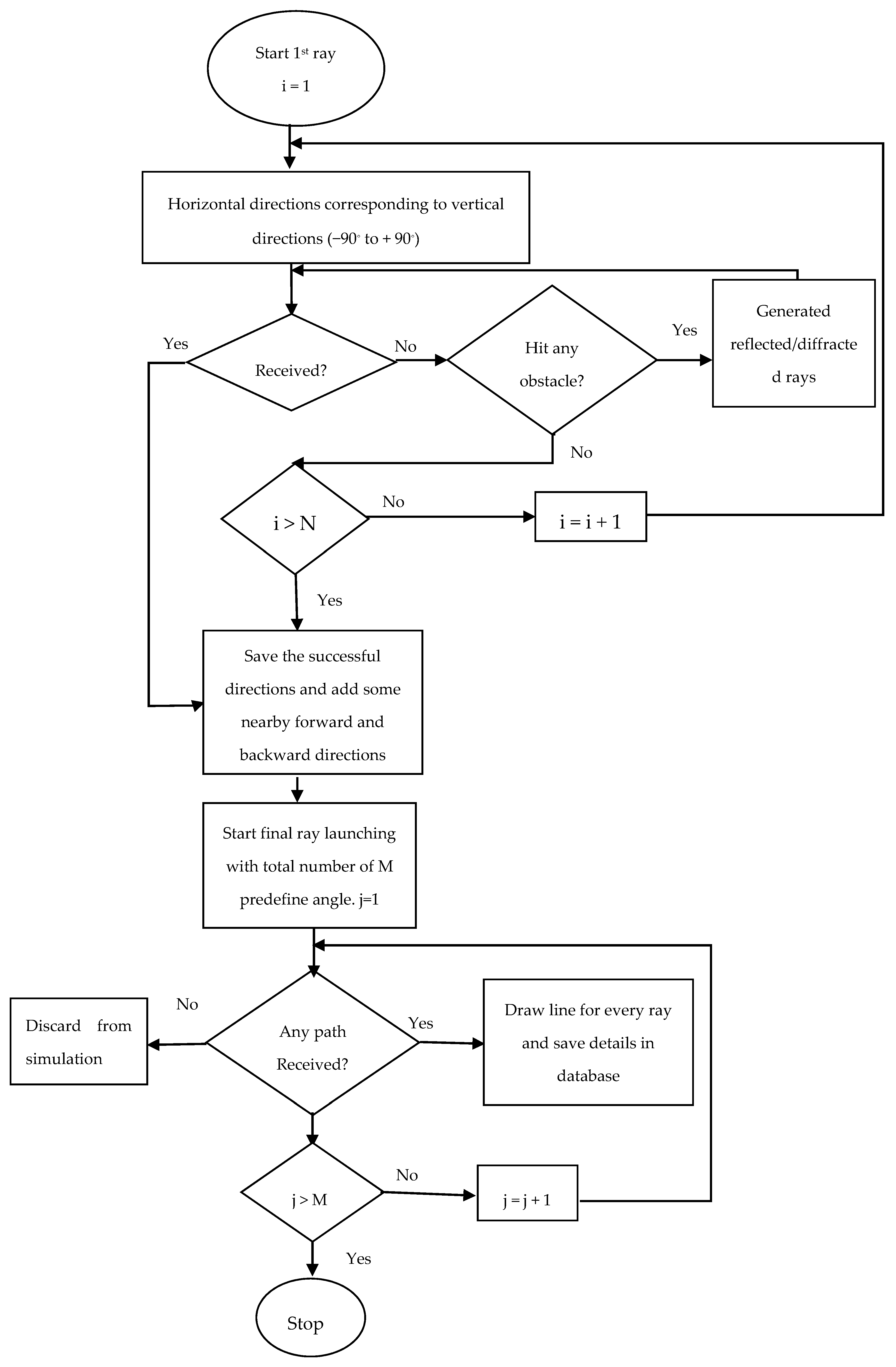
The main aim of this algorithm is to determine rays from the TX to the Rx efficiently. The fundamental idea of smart 3D RT is to trace rays from the TX to the Rx in four steps: pre-ray launch, ensuring more rays are in the potential area, final ray launch, and determination of ray reception.

• Firstly, the rays were launched at regular horizontal angle steps of (π/60) radian. For each of the horizontal angles, rays were also launched at regular vertical angle steps of (π/180) radian for pre-calculation to identify the angles whose rays successfully reached the Rx. In the existing method, the horizontal angle steps are used as (π/180) radian. As a result, almost three times more calculation in existing method with compare to the proposed method.
• Secondly, we refined the horizontal corresponding vertical angles directions by adding narrower additional angles for the forward and backward directions in order to ensure more precision rays at potentially successful directions.
• Thirdly, final ray launching at updated angles was conducted to include pre-determined potential directions.
• Fourthly, we traced rays throughout the receiver by applying the theory of transmission, reflection, and diffraction to determine the successful rays that reached the Rx.

The main advantages of our proposed smart 3D method are as follows. The number of launched rays were drastically minimized because the number of horizontal directions were reduced. Because of launched more rays in pre-defined and pre-calculated directions, more rays were captured by the receivers, which helped to lead to more accurate results.

Figure 1 shows the flowchart of the proposed smart RT method. The symbol N stands for the total number of launched rays for preprocessing. After preprocessing, together with additional unique forward and backward directions, the total horizontal direction-wise vertical directions are expressed by M.

The complexity of smart 3D RT is low, as only the pre-defined zone rays are launched. Because of the narrow launching zone, better accuracy is obtained with higher levels of reflection. Moreover, less computational time is needed. In conventional methods, more rays shoot in all directions, so the complexity of the calculations increase massively. The massive shooting takes place without knowing whether the rays will contribute to the Rx or not. Hence, the smart RT method is more efficient because of the pre-defined directions for ray launching.

4. Ray-Based Radio Wave Power Level Modelling

In the simulation, ray reflections and diffractions are sometimes accrued together before the ray reaches its destination. Under this circumstance, power level $E_n$ can be calculated by Equation (9).

$$E_n=E_{in}\left(Q_n\right)\left({\displaystyle \prod }_{i=0}^{a_n}{R}_{in}{A}_{rin}\right)\left({\displaystyle \prod }_{j=0}^{b_n}{T}_{jn}{A}_{tjn}\right)\left({\displaystyle \prod }_{m=0}^{c_n}{D}_{mn}{A}_{dmn}\right)e^{-jk{s}_n}$$

(9)

The terms $E_{in}\left(Q_n\right), a_n, b_n, c_n, R_{in}, T_{jn}, \mathrm{and} D_{mn}$ are the first scattering, number of reflections, number of transmissions, number of diffractions, associate dyadic reflection coefficient, associate dyadic transmission coefficient, and associate dyadic diffraction coefficient, respectively. The correlated spreading factors are symbolized by $A_{rin}, A_{tjn}, \mathrm{and} A_{dmnn}$. The traveled cumulative path of a ray is expressed by S_n. For reflections and diffraction phenomena every Rx received several ray paths. The receiver-wise total power level $E_{total}$ is the summation of each ray path power, which can be calculated by Equation (10).

$$E_{total}={\displaystyle \sum }_{n=0}^M E_{in}\left(Q_n\right)\left({\displaystyle \prod }_{i=0}^{a_n}{R}_{in}{A}_{rin}\right)\left({\displaystyle \prod }_{j=0}^{b_n}{T}_{jn}{A}_{tjn}\right)\left({\displaystyle \prod }_{m=0}^{c_n}{D}_{mn}{A}_{dmn}\right)e^{-jk{s}_n}$$

(10)

The total number of successful rays for a specific Rx is expressed by M. The TX power $P_t$, antenna pattern, and $Q_n$ is used to calculated $E_{in}\left(Q_n\right)$ by Equation (11).

$$E_{in}\left(Q_n\right)=\frac{E_0\sqrt{G_m^{\prime }}}{p_n} {\tilde{a}}_m$$

(11)

The $E_0=\sqrt{\frac{n_0}{4\pi }}{P}_t{G}_t$ is the power level that is ideally calculated from a 1-m distance from the TX. The symbols $n_0$, $G_t, G_m^{\prime }$, ${\tilde{a}}_m$, $Q_n,$ and $p_n$ are intrinsic impedance, antenna directivity, antenna gain, and polarization in the direction of $Q_n$, respectively. The $p_n$ expresses the distance between $Q_n$ and TX. The Vrn expresses voltage with respect to the Rx antenna and polarization. The Vrn is calculated using Equation (12).

$$V_{rn}=\sqrt{\frac{{\lambda }^2{G}_{rn}{R}_0}{4\pi }}\left({\mathrm{E}}_n.{\tilde{a}}_{rm}\right)e^{j\varphi }$$

(12)

The symbols $\lambda$, $G_{rn}$, $R_0$, ${\tilde{a}}_{rm}$, and $e^{j\varphi }$ are the wavelength, Rx gain, Rx impedance, Rx polarization, and fixed-phase shift, respectively. Finally, the Rx power level is calculated by Equation (13).

$$\begin{array}{l}{P}_r=\frac{{\left|{{\displaystyle \sum }}_{n=0}^M{V}_m\right|}^2}{R_0}\\ =\frac{{\lambda }^2}{4\pi n_0}{\left|{\displaystyle \sum _{n=0}^M}\left(E_n.{\tilde{a}}_{rn}\right)\sqrt{G_{rn}}\right|}^2\\ =\frac{{\lambda }^2}{4\pi n_0}\left|{\displaystyle \sum _{n=0}^M}\frac{E_0{e}^{-jk{s}_n}\sqrt{G_{rn}{G}_{tn}^{\prime }}}{P_n}{\tilde{a}}_{tn}\left({\displaystyle \prod _{i=0}^{a_n}}{R}_{in}{A}_{rin}\right)\left({\displaystyle \prod _{j=0}^{b_n}}{T}_{jn}{A}_{tjn}\right)\left({\displaystyle \prod _{m=0}^{c_n}}{D}_{mn}{A}_{dmn}\right){\tilde{a}}_{rn}\right|\end{array}$$

(13)

The total number of successful paths is symbolized by M.

5. Results Validation and Discussion

The measurement campaign was conducted on the ground floor of the Wireless Communication Center (WCC), which is situated at Universiti Teknologi Malaysia (UTM) at Johor Bahru Campus in Malaysia. The directional horn antenna was connected with an MG369xC model signal generator; its beamwidth (degrees), height (m), and operational frequency (GHz) values were 18, 2, and 28, respectively. Similarly, the omnidirectional receiver antenna was linked with an MS2720T model spectrum analyzer. The TX was placed in a fixed position in the WCC in Room 3, and measurements were started from 1-m away from the Rx. However, the antenna height was vital in coverage [14].

There are several methods to handle the rays; however, we used the most reputed 3D SB RT method and proposed a smart 3D RT method in this simulation. Outcomes from both the simulation methods were compared with actual measurements. The simulations were performed using measurement layouts which were developed in the in-house simulator.

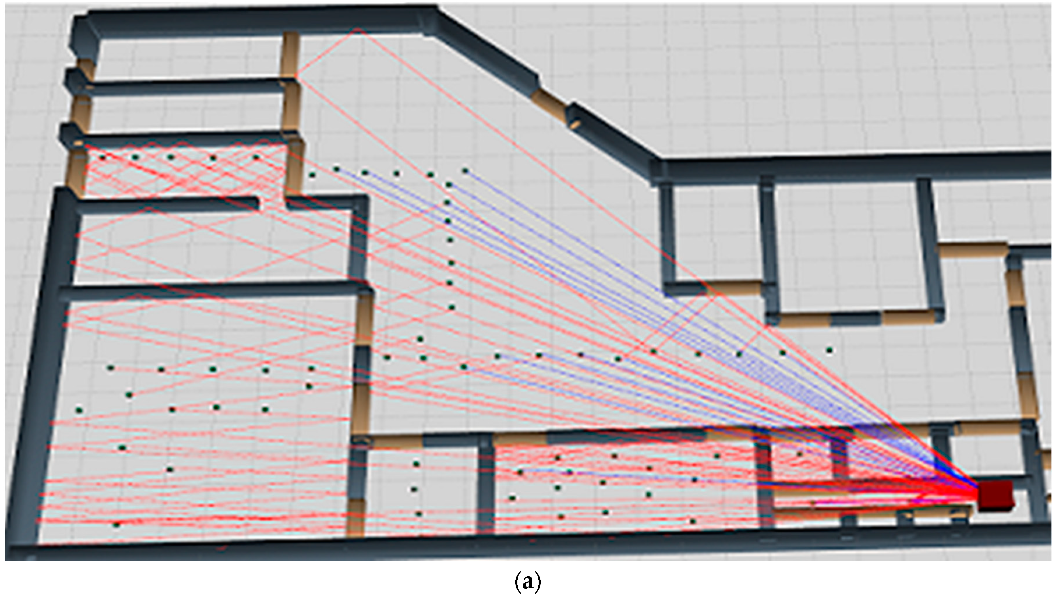
In the measurements, we covered 14 points, and all relevant simulated point information was presented in terms of path loss and power level. Figure 2 expresses the simulated LoS and NLoS paths’ visual representation. For both methods, the simulated path information was stored in the database. The relevant parameters and factors were used in the calculations. The receiver power level, path loss, etc., were calculated using mathematical functions.

The graphical comparison of measurement and simulation results for path loss and power level is shown in Figure 3. We calculated the path loss standard deviation using a standard formula to see how different the simulation path loss was from the measurements. As the standard deviation of path loss was calculated with the measurements data for all simulation points, it considers the average path loss error of the simulation. The 3D SB RT method path loss standard deviation was 4.00, with respect to the measurements. Among the 14 points, specifically Rx37, Rx70, Rx8, Rx9, Rx4, and Rx11 expressed good agreement with the 3D SB RT method. Similarly, for the 3D proposed smart RT method, the path loss standard deviation was 1.87 with respect to the measurements. In the 3D smart method simulation, almost all points except (Rx47, Rx8) expressed very good agreement with the measurements. For the SB RT method, the path loss standard deviation value was 2.13 dB higher than the proposed smart RT method, with respect to the measurements. In the path loss analysis, it was reported that our 3D smart method had achieved a better agreement with the measurements rather than the 3D SB RT method. Furthermore, we calculated the power level’s standard deviation using the standard formula to see how different the simulation’s power level was from the measurements. The standard deviation of the power level was calculated with the measurement data for all simulation points, so it considers the average power level error of the simulation. Here, in the 3D SB RT method, the power level’s standard deviation was 4.33 with respect to the measurements. From the 14 points, only Rx70, Rx37, and Rx34 expressed good agreement with the 3D SB RT method. Similarly, the 3D smart RT method’s power level’s standard deviation was 2.25, with respect to the measurements. Moreover, in the 3D smart method simulation, almost all points (except Rx7, Rx11, and Rx4) expressed very good agreement. However, for the indoor radio propagation prediction simulation, the power level standard below five was acceptable. But the simulation method had a smaller standard deviation with respect to the measurements, meaning that it was closer to the reality. The SB RT method’s power level’s standard deviation value was 2.08 dBm higher than the proposed smart RT’s, with respect to the measurements. In the power-level analysis, our 3D smart method achieved a better agreement with the measurements than the 3D SB RT method.

Figure 4 shows the comparison graph of the number of rays received using the 3D SB RT and the 3D smart RT methods. The comparison was performed between the 3D SB RT and the 3D smart method data, as the measurements were not able to generate this data. According to Figure 4, it was reported that in the 3D smart RT method, higher numbers of rays reached the Rx rather than the 3D SB RT method. In the RT, the richness of interactions and greater number of rays received by receivers indicates good modelling with a high level of accuracy. The lower standard deviation for path loss and power level in the 3D smart RT method fully justifies this finding.

Figure 5 shows the comparison graph of receiver ray propagation time for the SB RT and 3D smart RT methods. Most of the cases in the 3D SB RT method took a higher computational time compared to the 3D smart method. For this comparison purpose, both methods used the same high configured server with graphics card [15,16]. The 3D SB RT and 3D smart methods belong to the site-specific model family. However, the site-specific models provided, scenario wise, better propagation predictions in terms of accuracy than the empirical and stochastic models. In the 3D site-specific models, high-computational time is considered the main drawback. For this scenario, the smart method saved 27.29% of time over the conventional SB RT method. From this analysis, it is clear that our smart RT method is faster than the conventional method, and it has a good ability to overcome the site-specific model’s main drawback.

In this work, we improved ray launching to make the 3D smart RT method more capable, suitable, and intelligent. To achieve better coverage, the use of higher rays only in pre-defined directions is the key contribution of our method. From the results and discussions, it is clear that the proposed 3D smart RT method has a better contribution to radio propagation in terms of path loss, power level, propagation time, and coverage.

6. Conclusions

In this article, we offered a smart 3D RT method to investigate indoor radio propagation at 28 GHz. This method allows launching more rays in a pre-defined potential zone, which minimizes the computational complexity without reducing valid paths between the TX and the Rx. This path loss and power level were validated by measurement. Moreover, the coverage and propagation time results were better than those using the 3D SB RT method.

References

- Ericsson. Stockholm, Sweden. Ericsson Mobility Report. November 2014. Available online: https://www.ericsson.com/assets/local/mobility-report/documents/2014/ericsson-mobility-report-august-2014-interim.pdf (accessed on 6 January 2019).
- Forecast, C.V. Cisco Visual Networking Index: Global Mobile Data Traffic Forecast Update, 2016–2021 White Paper; Cisco Public Inf.: San Jose, CA, USA, 2017; pp. 1–35. [Google Scholar]
- Li, X.; Li, Y.; Li, B. The Diffraction Research of Cylindrical Block Effect Based on Indoor 45 GHz Millimeter Wave Measurements. Information 2017, 8, 50. [Google Scholar] [CrossRef]
- Smulders, P. Exploiting the 60 GHz band for local wireless multimedia access: Prospects and future directions. IEEE Commun. Mag. 2002, 40, 140–147. [Google Scholar] [CrossRef]
- Suzuki, Y.; Omiya, M. Computer simulation for a site-specific modeling of indoor radio wave propagation. In Proceedings of the IEEE Region 10 Conference (TENCON), Singapore, 22–25 November 2016; pp. 123–126. [Google Scholar] [CrossRef]
- Geok, T.K.; Hossain, F.; Chiat, A.T.W. A novel 3D ray launching technique for radio propagation prediction in indoor environments. PLoS ONE 2018, 13, e0201905. [Google Scholar] [CrossRef] [PubMed]
- Molish, A. Wireless communications. IMA Vol. Math. Appl. 2011. [Google Scholar] [CrossRef]
- Iskander, M.F.; Yun, Z. Propagation prediction models for wireless communication systems. IEEE Trans. Microw. Theory Tech. 2002, 50, 662–673. [Google Scholar] [CrossRef]
- Yun, Z.; Zhang, Z.; Iskander, M.F. A raytracing method based on triangular grid approach and application to propagation prediction in urban environments. IEEE Trans. Antennas Propag. 2002, 50, 750–758. [Google Scholar]
- Sulyman, I.; Nassar, A.T.; Samimi, M.K.; MacCartney, G.R., Jr.; Rappaport, T.S.; Alsanie, A. Radio propagation path loss models for 5G cellular networks in the 28 GHz and 38 GHz millimeter-wave bands. IEEE Commun. Mag. 2014, 52, 78–86. [Google Scholar] [CrossRef]
- Shi, D.; Tang, X.; Wang, C. The acceleration of the shooting and bouncing ray tracing method on GPUs. In Proceedings of the 2017 General Assembly and Scientific Symposium of the International Union of Radio Science (URSI GASS), Montreal, QC, Canada, 19–26 August 2017; pp. 1–3. [Google Scholar] [CrossRef]
- Geok, T.K.; Hossain, F.; Kamaruddin, M.N.; Rahman, N.Z.A.; Thiagarajah, S.; Chiat, A.T.W.; Liew, C.P. A Comprehensive Review of Efficient Ray-Tracing Techniques for Wireless Communication. Int. J. Commun. Antenna Propag. 2018, 8, 123–136. [Google Scholar] [CrossRef]
- Yun, Z.; Iskander, M.F. Ray Tracing for Radio Propagation Modeling: Principles and Applications. IEEE Access 2015, 3, 1089–1100. [Google Scholar] [CrossRef]
- Hong, Q.; Zhang, J.; Zheng, H.; Li, H.; Hu, H.; Zhang, B.; Lai, Z.; Zhang, J. The Impact of Antenna Height on 3D Channel: A Ray Launching Based Analysis. Electronics 2018, 7, 2. [Google Scholar] [CrossRef]
- Hossain, F.; Geok, T.K.; Rahman, T.A.; Hindia, M.N.; Dimyati, K.; Abdaziz, A. Indoor Millimeter-Wave Propagation Prediction by Measurement and Ray Tracing Simulation at 38 GHz. Symmetry 2018, 10, 464. [Google Scholar] [CrossRef]
- Hossain, F.; Geok, T.K.; Rahman, T.A.; Hindia, M.N.; Dimyati, K.; Ahmed, S.; Tso, C.P.; Abd Rahman, N.Z. An efficient 3-D ray tracing method: prediction of indoor radio propagation at 28 GHz in 5G network. Electronics 2019, 8, 286. [Google Scholar] [CrossRef]
© 2019 by the authors. Licensee MDPI, Basel, Switzerland. This article is an open access article distributed under the terms and conditions of the Creative Commons Attribution (CC BY) license (http://creativecommons.org/licenses/by/4.0/).