Modeling and Optimization of Gaseous Thermal Slip Flow in Rectangular Microducts Using a Particle Swarm Optimization Algorithm

Abstract

In this study, pressure-driven flow in the slip regime is investigated in rectangular microducts. In this regime, the Knudsen number lies between 0.001 and 0.1. The duct aspect ratio is taken as $0\le \epsilon \le 1$. Rarefaction effects are introduced through the boundary conditions. The dimensionless governing equations are solved numerically using MAPLE and MATLAB is used for artificial neural network modeling. Using a MAPLE numerical solution, the shear stress and heat transfer rate are obtained. The numerical solution can be validated for the special cases when there is no slip (continuum flow), $\epsilon =0$ (parallel plates) and $\epsilon =1$ (square microducts). An artificial neural network is used to develop separate models for the shear stress and heat transfer rate. Both physical quantities are optimized using a particle swarm optimization algorithm. Using these results, the optimum values of both physical quantities are obtained in the slip regime. It is shown that the optimal values ensue for the square microducts at the beginning of the slip regime.

1. Introduction

1.1. Rarefied Gas Flows

Flows in microducts are found in microelectromechanical systems, nanotechnology applications, therapeutic and superhydrophobic microchannels, low-pressure environments, biochemical applications and cryogenics. The rarefaction effect can be found in microchannels and can be expressed in terms of the Knudsen number. In this case, the deviations from continuum behavior are smaller. Therefore, the Navier–Stokes equations can be employed with slip boundary conditions. The difference between a fully developed flow in a rectangular duct and in a microchannel is that a rectangular microduct needs 2D analysis, whereas a microchannel entail a one-dimensional analysis.

Generally, the Navier–Stokes equations can be solved with slip boundary conditions at the microduct walls [1,2]. Previous studies [1,2] found that the solutions were validated by the experimental data in several microchannel flows. Otherwise, significant departures were observed between the numerical and experimental results without applying the slip conditions. Ameel et al. [3] confirmed the statement of Reference [1,2]. Zade et al. [4] considered variable physical properties and investigated thermal features of developing flows in rectangular microchannels. They employed a collocated finite volume method and studied several channel dimensions for different values of slip parameters. They found that variable properties show substantial changes in flow behavior. Ghodoossi and Eğrican [5] determined the heat transfer rate using an integral method. They predicted thermal features for isothermal boundary conditions. They noticed that, for any aspect ratio, the rarefaction had obvious effects on the heat transfer.

The effects of rarefaction on the Nusselt numbers were investigated by Hettiarachchi et al. [6] for thermally developing flows. They noticed that these Nusselt numbers increased with the slip velocity, and decline with the thermal jump boundary condition. The slip flow forced convection in rectangular microchannels was also considered by Yu and Ameel [7]. It was found that the velocity slip and aspect ratio enhance heat transfer. For rarefied gas flows, Renksizbulut et al. [8] observed exceptionally large reductions in the friction and heat transfer coefficients. They found that these coefficients are insensible to rarefaction effects in corner-dominated flows. Tamayol and Hooman [9] analyzed microchannels of polygonal, rectangular, and rhombic cross-sections and showed that the Poiseuille numbers decrease with increasing aspect ratios and Knudsen numbers for rectangular channels. Hooman [10] investigated forced convection in microducts using a superposition approach for both thermal boundary conditions and demonstrated that their results were valid for several cross-sections. Sadeghi and Saidi [11] considered the rarefaction effects in two different microgeometries and demonstrated that for both geometries, the Brinkman number reduced the heat transfer rate. In fact, the Brinkman number measures the viscous heating effects with reference to the heat conduction. They also developed a correlation for the Nusselt number.

Yovanovich and Khan [12] developed several slip flow models for microchannels of different cross-sections. The slip flow in circular and other cross-sections was investigated by a number of authors, including References [13,14,15,16]. They developed different models for envisaging the friction factor under both developing and fully developed conditions. Duan and Muzychka [13,14] proposed a simple model to predict the Poiseuille numbers in these microchannels. Duan and Muzychka [15] considered slip flow in the entrance of circular and parallel plate microchannels and noticed that the Poisseuille number depends on the Knudsen number. Yovanovich and Khan [16] modeled the Poiseuille flow in long channels of different cross-sections. Ebert and Sparrow [17] analyzed abstemiously rarefied gas flows in different ducts and noticed that the velocity flattened and the friction lessened due to the slip parameter.

Baghani et al. [18] treated rarefaction effects in microducts of different cross-sections and obtained Nusselt numbers under isothermal boundary condition. They tabulated Nusselt numbers for the entire slip flow range of the Knudsen number. Wang [19] considered the slip flow under an isothermal boundary condition in different ducts. It was found that both hydrodynamic and thermal boundary conditions have substantial effects on both the Poiseuille and Nusselt numbers. Also, both parameters showed an opposite trend with an increasing velocity slip. Beskok and Karniadakis [20] considered internal rarefied gas flows and presented mathematical models for different regimes. To account for heat transfer from the surface, they suggested a new boundary condition and demonstrated that it is applicable in all flow regimes. Yovanovich and Khan [21] proposed compact models for isothermal, incompressible slip flows in different microchannels. They used the principle of superposition in the analysis and introduced new flow parameters. They compared their results with previous numerical results for different cross-sections and found them in a very good agreement. Klášterka et al. [22] obtained analytical and numerical solutions for the flow variables and demonstrated the effect of slip parameters on the friction and heat transfer coefficients.

The above literature survey reveals that there are only a few studies related to rectangular microducts. However, there has been no study where the numerical models are developed using an artificial neural network (ANN) and are optimized for the duct geometry. This fact inspires us to model our numerical results using ANN and to acquire optimized values of friction factors and Nusselt numbers using a particle swarm optimization algorithm.

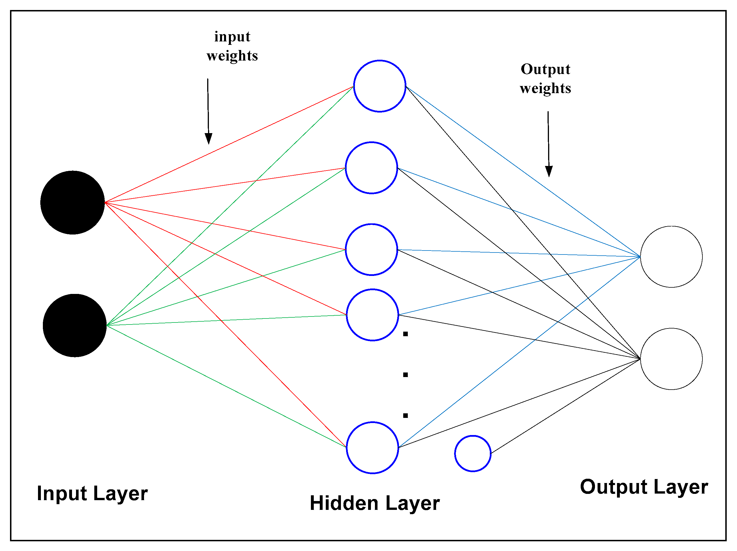
1.2. Artificial Neural Networks

Artificial neural networks (ANNs) are mathematical models, which are inspired by biological nervous systems [23,24]. The multilayer perceptron neural network (MLPNN) is one of the widely known feedforward neural networks. MLPNNs have three types of layers, which are the input layer, the hidden layers, and the output layer. Figure 1 shows the structure of MLPNN [25,26].

The activation function is defined as an output of a node or a neuron and can be written as:

$$Y=\frac{1}{1+e^{-x}}$$

(1)

where x is an input value from the input layer. Supervised learning of ANNs is useful for improving the performance of ANN models. Several algorithms are used for the training to find the best parameters of the neural networks [27,28]. The optimization algorithms are used to find the best values for inputs and output weights that are parameters of MLPNNs. In this study, the particle swarm optimization (PSO) algorithm is used to train the neural networks, because it is one of the most effective meta-heuristic algorithms used for optimization problems. Equation (2) is the sum of squared error (SSE) function, which was used as a fitness function for testing the performance of the ANNs [25].

$$SEE={\displaystyle \sum }{\left(Actual output-target output\right)}^2$$

(2)

where the $target output$ values are determined by Equation (3), while the $Actual output$ values are determined by the neural network (NN) output values.

$$Output\left(y_k\right)={\displaystyle \sum }_{j=1}^m{\displaystyle \sum }_{i=1}^n{w}_{jk}{\displaystyle \sum }_{k=1}^s{w^{\prime }}_{ki}\frac{1}{1+e^{-x_j}}$$

(3)

where n, m, k, $w_{jk}$, and $w{\prime }_{ki}$ represent the number of neurons in the hidden layer, number of input data, number of neurons in input layer, number of neurons in output layer, input weight—which is between the input neurons and hidden neurons—and output weight, which is between the hidden neurons and output neurons, respectively.

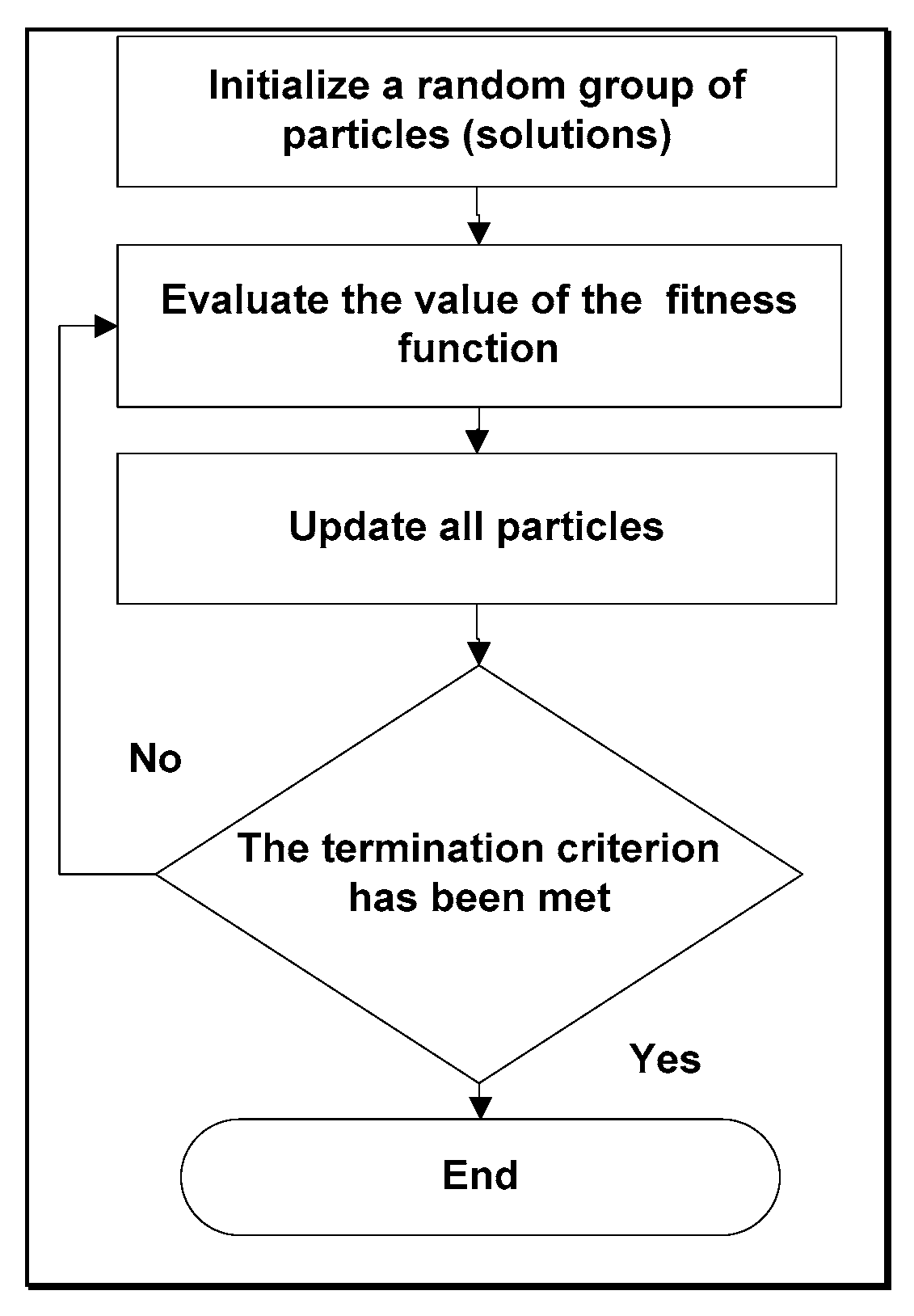
1.3. Particle Swarm Optimization Algorithm

The principle of the particle swarm optimization (PSO) algorithm came from the ideas of the social behavior of bird flocks, as well as from the shoaling behavior of fish [27,28,29]. All solution members of the algorithm are called particles. The particle flies by updating its velocity vectors v and position x, by using Equations (4) and (5), respectively [30].

$$\begin{array}{ll}{v}_{ik}\left(t+1\right)=& v_{ik}\left(t\right)+c_1\ast r_{1k}\left(t\right)\ast \left(y_{ik}\left(t\right)-x_{ik}\left(t\right)\right)+c_2\\ & \ast r_{2k}\left(t\right)\ast (\widehat{y_k}\left(t\right)-x_{ik}\left(t\right))\end{array}$$

(4)

$$x_i\left(t+1\right)=x_i\left(t\right)+v_i\left(t+1\right)$$

(5)

where $x_i\left(t\right)$, $v_i\left(t\right)$, $y_i\left(t\right)$, and $\widehat{y_k}\left(t\right)$ represent the position at time t, the velocity at time t, the best personal position ($p^{best}$) at time t, and the global best position ($g^{best}$) of population at time t respectively, whereas $c_1$ and $c_2$ are the learning factors of ($p^{best}$) in interval between 0 and 2 and r₁ and r₂ are the random numbers in the interval 0 to 1.

It is important to note that the other particles follow the performance of the best particle [31,32,33,34]. In addition, each particle keeps the best position that it has achieved so far. The flowchart of Figure 2 shows the steps of the present PSO algorithm [27,32,35].

Thus, the particles should move towards the best directions, and utilize useful information from other particles along with the best particles [30,35].

In this study, the algorithm was used to find the optimal values of the Nusselt number (Nu) and Poiseuille number (Po) corresponding to the aspect ratio and the Knudsen number in the slip flow regime. The number of the iterations was set as 50, with initial populations 60, and c₁ = c₂ = 0.05 [30].

To the best of our knowledge, most of the existing analytical solutions for slip flows are limited to fluid flow in rectangular ducts. There is a lack of literature related to heat transfer in microducts. Furthermore, there is no study related to ANN modeling and optimization of pressure drop and heat transfer in microducts. The aim of this paper was to cover these aspects.

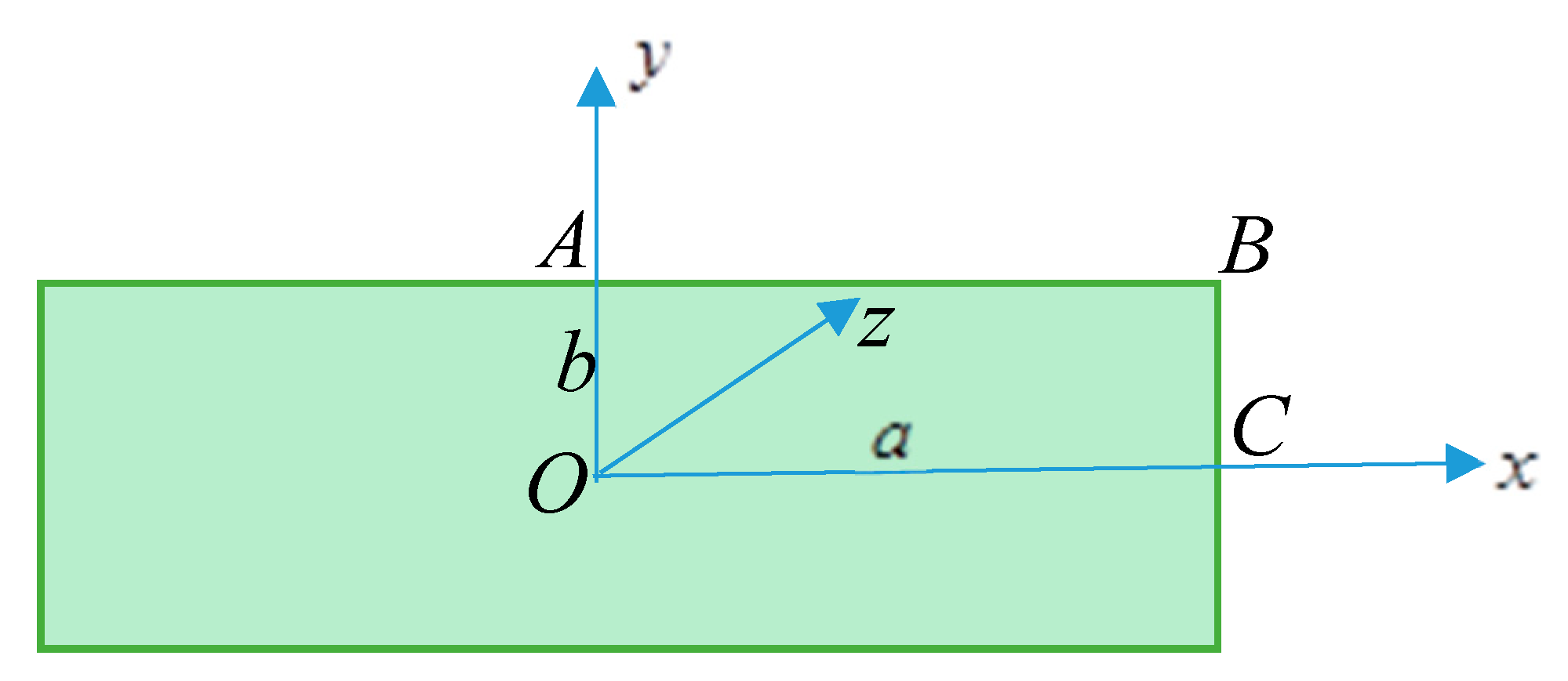
2. Mathematical Model

2.1. Hydrodynamic Analysis

Let us consider a fully developed flow in a rectangular duct, as shown in Figure 3. The semi-major and -minor axes are taken as $a$ and $b$ along the x- and y-axes, respectively. The aspect ratio is $\epsilon =b/a$. The gas is assumed to flow along the z-axis. The momentum equation for the flow in a microduct can be written as:

$$\frac{{\partial }^{2}u}{\partial x^2}+\frac{{\partial }^{2}u}{\partial y^2}=-\frac{1}{\mu }\frac{dP}{dz}$$

(6)

which is a 2D equation for the axial velocity $u$, uniform gas viscosity $\mu$ and constant pressure gradient $dP/dz$. Due to double symmetry, only the OABCO is selected for the simulation. The velocity slip and symmetry boundary conditions for this problem can be written as:

$$u=-\lambda \frac{2-{\sigma }_v}{{\sigma }_v}{\frac{\partial u}{\partial y}|}_{y=b}\hspace{1em}u=-\lambda \frac{2-{\sigma }_v}{{\sigma }_v}{\frac{\partial u}{\partial x}|}_{x=a}$$

(7)

and:

$${\frac{\partial u}{\partial y}|}_{y=0}=0;\hspace{1em}{\frac{\partial u}{\partial x}|}_{x=0}=0$$

(8)

where ${\sigma }_v$ is the tangential–momentum accommodation coefficient, which lies between 0.9 and 1, and $\lambda$ is the mean free path. If $A$ is the area of cross-section and $P$ is the perimeter of the duct, then the hydraulic diameter, $D_h$ can be written as:

$$D_h=4A/P=4b/(1+\epsilon )$$

(9)

At this stage, it is convenient to define the Knudsen number (the measure of rarefaction effects) as follows:

$$Kn=\lambda /D_h\hspace{1em}\Rightarrow \lambda =4bKn/1+\epsilon$$

(10)

Following Ebert and Sparrow [17], Equations (6)–(8) can be non-dimensionalized as follows.

Let:

$$\xi =x/a,\eta =y/b$$

(11)

The dimensionless momentum equation can be written as:

$${\epsilon }^2\frac{{\partial }^{2}u}{\partial {\xi }^2}+\frac{{\partial }^{2}u}{\partial {\eta }^2}=-1$$

(12)

where the axial velocity u is normalized with $u_o=\left(\frac{b^2}{\mu }\right)\left|\frac{dP}{dz}\right|$. Using Equation (11), dimensionless boundary conditions can be written as:

$$\begin{array}{l}u=-\frac{4Kn}{1+\epsilon }\frac{2-{\sigma }_v}{{\sigma }_v}{\frac{\partial u}{\partial \eta }|}_{\eta =1};\hspace{1em}0\le \xi <1\\ u=-\frac{4\epsilon Kn}{1+\epsilon }\frac{2-{\sigma }_v}{{\sigma }_v}{\frac{\partial u}{\partial \xi }|}_{\xi =1};\hspace{1em}0\le \eta <1\\ {\frac{\partial u}{\partial \eta }|}_{\eta =0}=0;\hspace{1em}0\le \xi <1;\hspace{1em}{\frac{\partial u}{\partial x}|}_{\xi =0}=0;\hspace{1em}0\le \eta <1\end{array}$$

(13)

The mean velocity in the duct is defined as:

$$\overline{u}=u_0{\displaystyle {\int }_0^1}{\displaystyle {\int }_0^{1}u(\xi ,\eta )\cdot d\xi }\cdot d\eta$$

(14)

The Poiseuille number $Po$ is defined as:

$$Po=c_f\cdot {\mathrm{Re}}_{D_h}$$

(15)

where $c_f={\overline{\tau }}_w/0.5\rho {\overline{u}}^2$ is the coefficient of friction and ${\mathrm{Re}}_{D_h}=\overline{u}{D}_h/\nu$ is the Reynolds number, based on mean velocity. For a fully developed flow, the force balance on a control volume of width $dz$ gives:

$$-A\cdot dp={\overline{\tau }}_{w}Pdz\Rightarrow {\overline{\tau }}_w=\left(dp/dz\right)\left(D_h/4\right)$$

(16)

Thus, the dimensionless shear stress can be expressed in terms of the Poiseuille number $Po$:

$$Po=-\frac{32}{{\left(1+\epsilon \right)}^2}\cdot \frac{1}{\left(\overline{u}/u_0\right)}$$

(17)

where $\overline{u}/u_0$ is the dimensionless average axial velocity in the microduct and can be determined from Equation (14).

2.2. Thermal Analysis

For fully thermally developed and steady flow in the rectangular microducts, the energy equation is given by:

$$\frac{k_f}{\rho c_p}\left(\frac{{\partial }^{2}T}{\partial x^2}+\frac{{\partial }^{2}T}{\partial y^2}\right)=u\frac{\partial T}{\partial z}$$

(18)

with temperature jump and symmetry boundary conditions:

$$\begin{array}{l}T-T_w=-\frac{\lambda }{\mathrm{Pr}}\frac{2-{\sigma }_t}{{\sigma }_t}\frac{2\gamma }{1+\gamma }{\frac{\partial T}{\partial y}|}_{y=b}\hspace{1em}\\ T-T_w=-\frac{\lambda }{\mathrm{Pr}}\frac{2-{\sigma }_t}{{\sigma }_t}\frac{2\gamma }{1+\gamma }{\frac{\partial T}{\partial x}|}_{x=a}\end{array}$$

(19)

and:

$${\frac{\partial T}{\partial y}|}_{y=0}=0\hspace{1em}{\frac{\partial T}{\partial x}|}_{x=0}=0$$

(20)

where $\mathrm{Pr}$ is the Prandtl number for the selected gas, ${\sigma }_t$ is the energy accommodation coefficient, and $\gamma$ is the ratio of specific heats of gas.

Using Equation (11), the energy balance in the flow direction can be written as:

$$\frac{k_f}{\rho c_p}\left({\epsilon }^2\frac{{\partial }^{2}T}{\partial {\xi }^2}+\frac{{\partial }^{2}T}{\partial {\eta }^2}\right)=u\frac{b^{2}Q}{4ab\rho c_p\overline{u}}$$

(21)

or:

$${\epsilon }^2\frac{{\partial }^{2}T}{\partial {\xi }^2}+\frac{{\partial }^{2}T}{\partial {\eta }^2}=\frac{u}{\overline{u}}\frac{\epsilon }{4}\frac{Q}{k_f}$$

(22)

where Q is the total energy per unit length of the duct and is assumed to be constant. Using $\theta =(T-Tw)/(Q/k_f)$, Equation (22) can be written as:

$${\epsilon }^2\frac{{\partial }^2\theta }{\partial {\xi }^2}+\frac{{\partial }^2\theta }{\partial {\eta }^2}=\frac{u}{\overline{u}}\frac{\epsilon }{4}$$

(23)

with transformed boundary conditions [17]:

$$\begin{array}{l}\theta =-\frac{4}{1+\epsilon }\frac{Kn}{\mathrm{Pr}}\frac{2-{\sigma }_t}{{\sigma }_t}\frac{2\gamma }{1+\gamma }{\frac{\partial \theta }{\partial \eta }|}_{\eta =1};\hspace{1em}0\le \xi <1\\ \theta =-\frac{4\epsilon }{1+\epsilon }\frac{Kn}{\mathrm{Pr}}\frac{2-{\sigma }_t}{{\sigma }_t}\frac{2\gamma }{1+\gamma }{\frac{\partial \theta }{\partial \xi }|}_{\xi =1};\hspace{1em}0\le \eta <1\\ {\frac{\partial \theta }{\partial \eta }|}_{\eta =0}=0;\hspace{1em}0\le \xi <1;\hspace{0.17em}\hspace{1em}{\frac{\partial \theta }{\partial \xi }|}_{\xi =0}=0;\hspace{1em}0\le \eta <1\end{array}\}$$

(24)

For a constant temperature jump condition, the Nusselt number can be defined as:

$$N{u}_T=\frac{{\partial T/\partial y|}_{\mathrm{wall}}}{T-T_{\mathrm{wall}}}$$

(25)

2.3. Solution Procedure

The solution procedure comprises three steps. In the first step, the numerical values of the Nu and Po numbers are determined, corresponding to different values of $\epsilon$ and $Kn$ by solving the governing Equations (12) and (23) by a finite difference method using MAPLE, and numerical data was obtained. In the second step, the back-error-propagation algorithm is employed to train a multi-layer perceptron neural network (MLPNN) using the neural network toolbox in MATLAB. There are two inputs, namely, the aspect ratio $\epsilon$ and the Knudsen number $Kn$. The corresponding outputs are the predicted values of the Nu and Po numbers, where each output is represented by a separate model. In each model, different input, hidden and output neurons are used. Finally, the results are optimized using PSO algorithm in order to find the optimal values of Nu and Po without gaining to the numerical values. Accordingly, the dimensionless partial differential equations will not use again in any stage of our work. As a result, the PSO algorithm uses neural network models to obtain the optimum values of Nu and Po.

3. Results and Discussion

The numerical values of Poiseuille numbers for forced convection in microducts were compared with the available data for different values of $Kn$ in

Table 1. Comparison of the Poiseuille numbers for forced convection when $Kn=0.1$.

$\mathit{\epsilon }$	Morini et al. [36]	Sadeghi et al. [37]	Present Results
0.2	9.46	9.464	9.519
0.4	8.65	8.654	8.721
0.6	8.25	8.248	8.331
0.8	8.08	8.076	8.178
1	8.04	8.033	8.159

,

Table 2. Comparison of numerical and exact values of $Po$ when $Kn=0.001$.

$\mathit{\epsilon }$	Numerical	Exact [38]	% Difference
0.001	24.031	23.7	1.3774
0.01	23.743	23.41	1.4025
0.02	23.432	22.24	5.0871
0.1	21.259	20.95	1.4535
0.2	19.182	18.89	1.5223
0.3	17.641	17.36	1.5929
0.4	16.514	16.24	1.6592
0.5	15.712	15.43	1.7948
0.6	15.164	14.87	1.9388
0.7	14.811	14.5	2.0998
0.8	14.608	14.28	2.2453
0.9	14.519	14.17	2.4037
1	14.514	14.14	2.5768

and

Table 3. Comparison of numerical and exact values of $Po$ when $Kn=0.1$.

$\mathit{\epsilon }$	Numerical	Exact [38]	% Difference
0.001	10.944	10.9	0.402
0.01	10.862	10.82	0.3867
0.02	10.773	10.47	2.8126
0.1	10.139	10.09	0.4833
0.2	9.519	9.46	0.6198
0.3	9.056	9	0.6184
0.4	8.721	8.66	0.6995
0.5	8.487	8.41	0.9073
0.6	8.331	8.25	0.9723
0.7	8.233	8.14	1.1296
0.8	8.178	8.08	1.1983
0.9	8.157	8.04	1.4344
1	8.159	8.04	1.4585

. The comparison showed excellent agreement with the available data. The predicted values of the Nusselt numbers are also provided in

Table 4. Numerical values of $Nu$ for different values of $Kn$.

$\mathit{\epsilon }$	$\mathit{K}\mathit{n}=0.001$	$\mathit{K}\mathit{n}=0.05$	$\mathit{K}\mathit{n}=0.1$
0.001	6.1658	1.4213	0.7164
0.25	5.1047	1.7625	1.0819
0.35	4.6786	1.8996	1.2287
0.5	4.0394	2.1051	1.4488
0.65	3.8048	2.1830	1.5590
0.75	3.6485	2.2348	1.6325
0.85	3.6156	2.2745	1.6816
1	3.5662	2.3341	1.7552

for different values of $\epsilon$ and $Kn$. To build the NN models, 70% of data was used as the training data, 15% as the testing data, and 15% as the validation data. In NN MATLAB tools, the back-error-propagation algorithm (an optimization algorithm) was used to determine the best models that have the optimal errors. These models were based on the mean squared error function of MSE = 0.00020768 and MSE = 0.00022112 for the two models, respectively, as shown in Figure 4 and Figure 5. The figures show that the best validation performance, in terms of the mean squared error function, were found after 187 and 452 iterations, respectively.

The correlation coefficients of the models are shown in Figure 6 and Figure 7. As expected, the correlation coefficient of the models was greater than 0.95. In addition, Figure 6 and Figure 7 show a significant convergence between the real values and the corresponding values that resulted from models. Accordingly, there was enough support to believe that the models were suitable to find the estimated values of the Nu and Po numbers. In addition, the coefficient of determination of the models was more than 0.99, which meant that both models could represent whole target data.

For optimization, the PSO algorithm was used to find the optimal values of Po and Nu, based on NN models. The optimal values of Po and Nu were achieved when $\epsilon =1$, and $Kn=0.001$. The behavior of Po and Nu values in the PSO algorithm is shown in Figure 8 and Figure 9. The optimal values of the curves were determined when the curves became stable. Accordingly, the optimal values for Nu and Po were found in iteration number 4 and 10, respectively. Note that, the data set values were converted into z-score values for use in the neural network toolbox in MATLAB.

4. Conclusions

In this study, the slip flow and heat transfer were investigated in rectangular microducts. The dimensionless governing partial differential equations with slip boundary conditions were solved numerically using MATLAB. The numerical data were used successfully for building ANN models. The outputs of the models were the corresponding Poiseuille Po and Nusselt Nu numbers to the input values $\epsilon$ and $Kn$. The main outcomes of the study were:

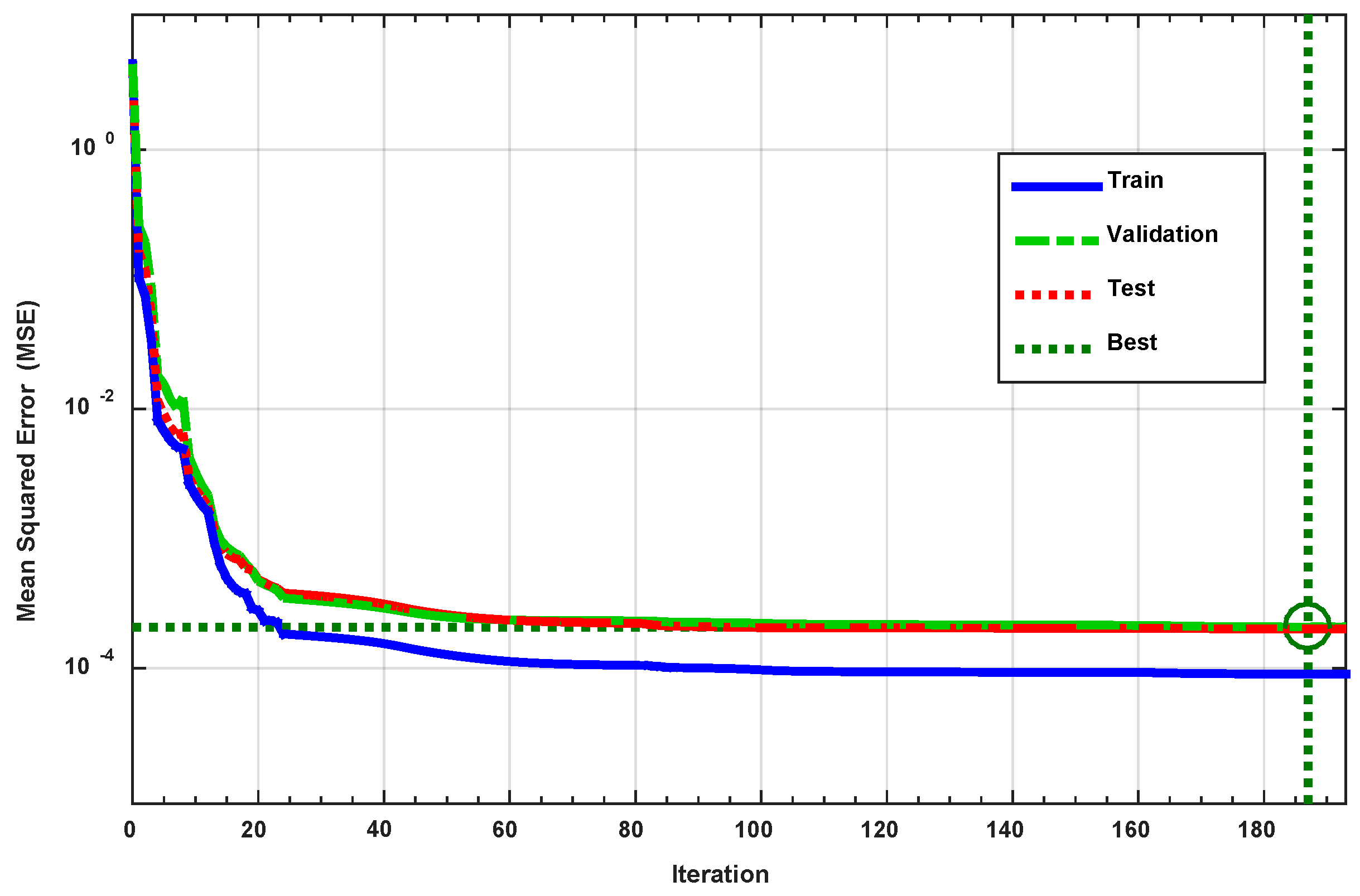
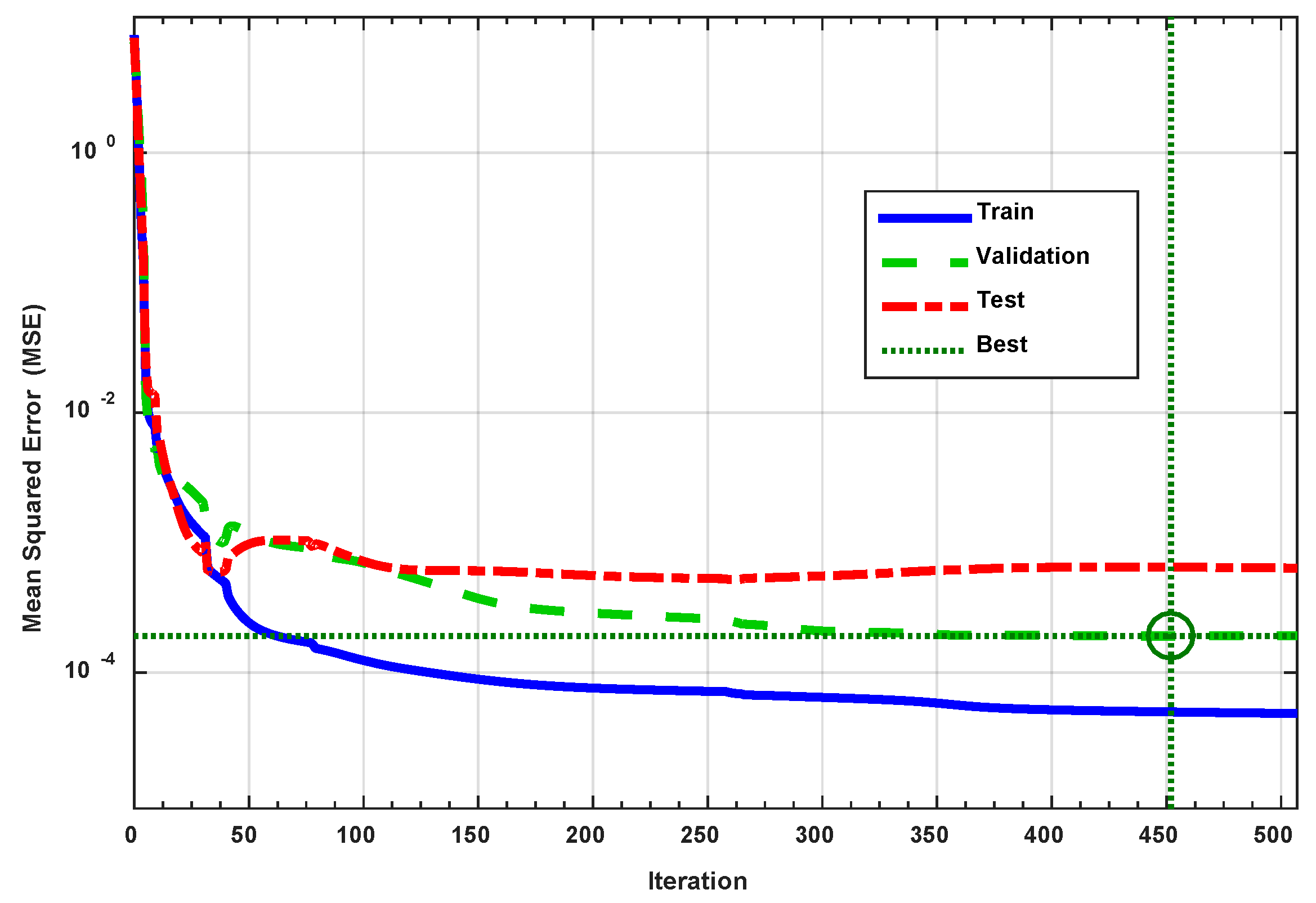
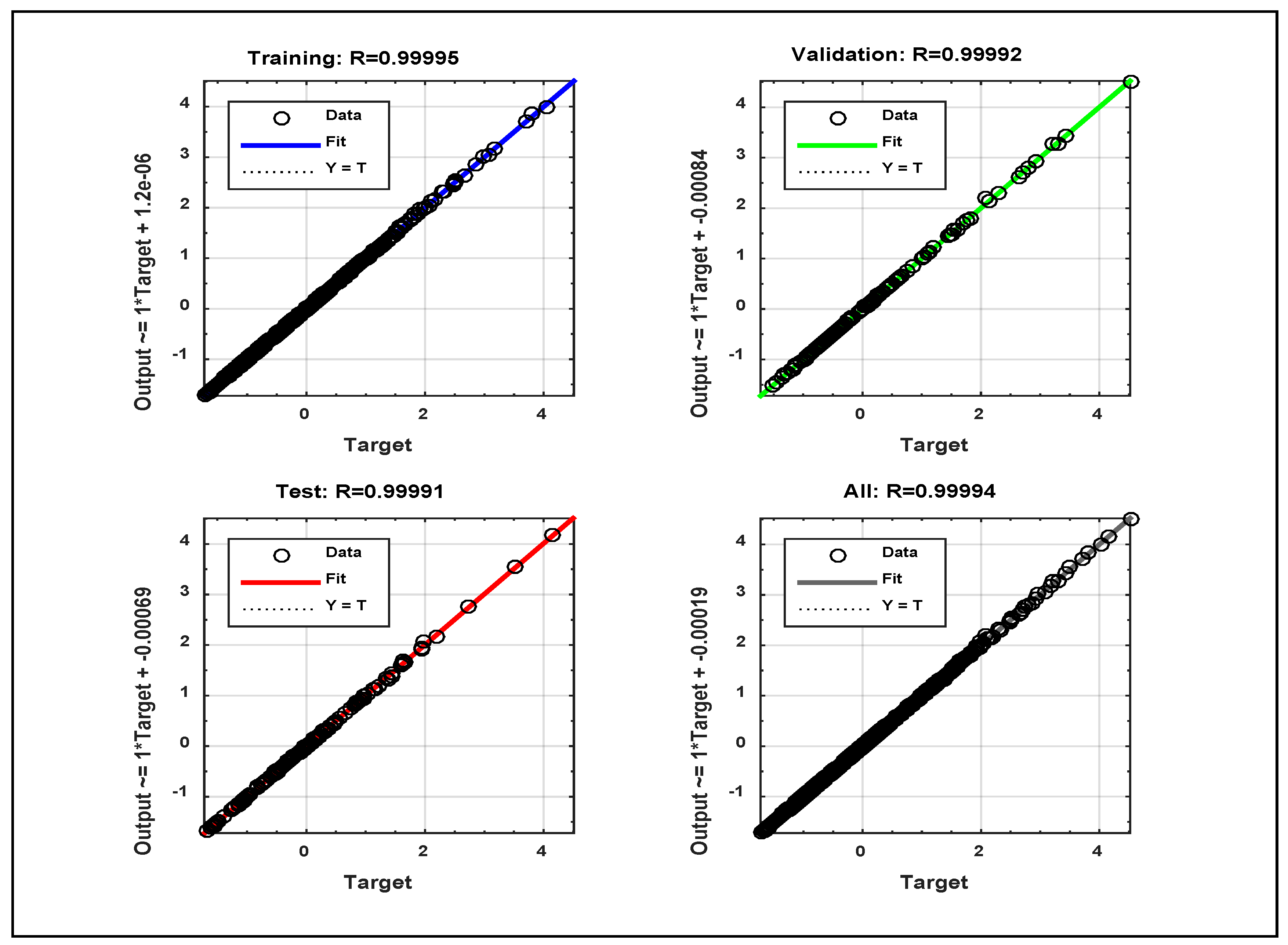
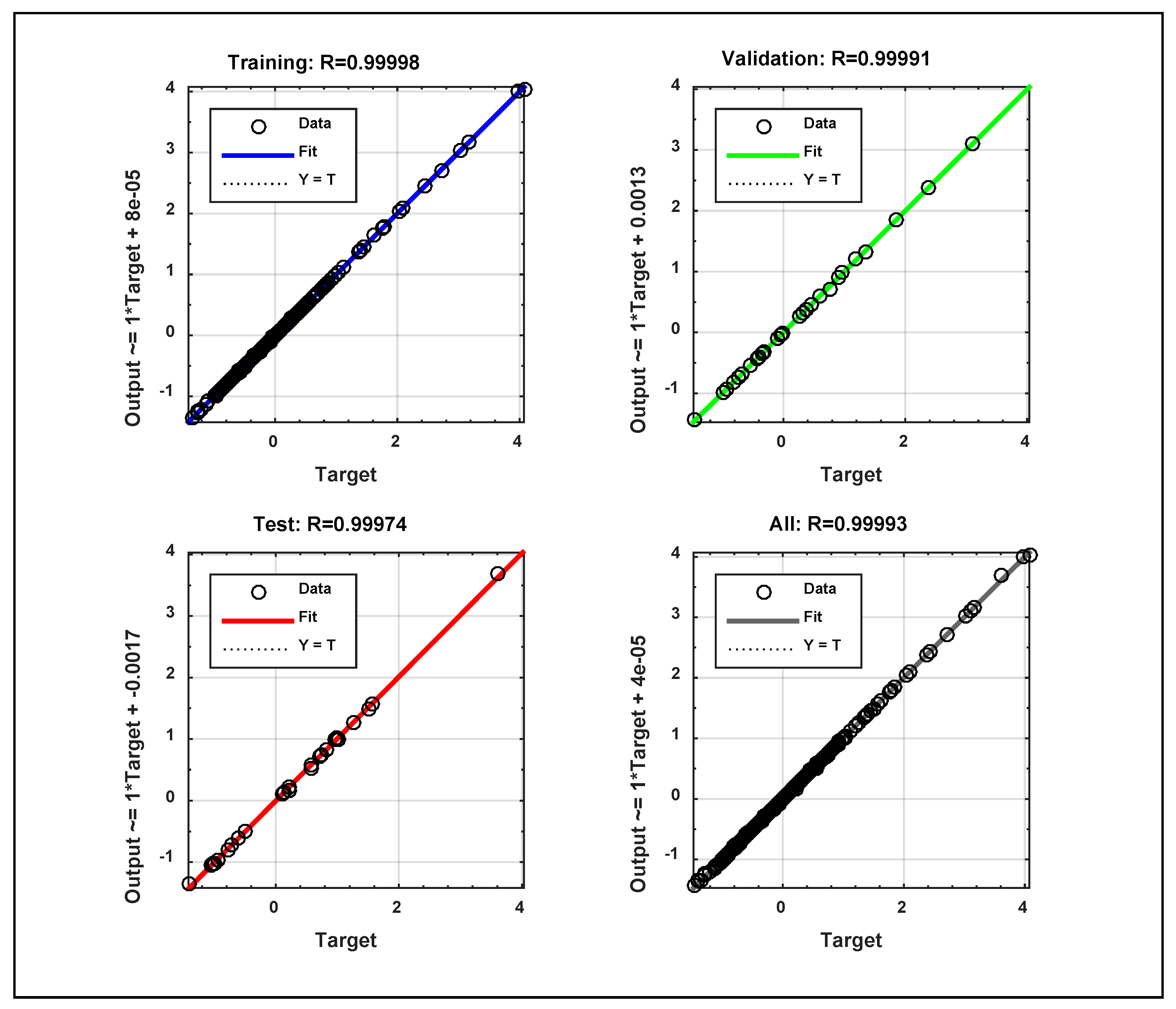
• The small tolerance values for the mean squared error function values and a very close correlation coefficient of 1 in the NN models proved that the NN models were suitable to use for predicting the Poiseuille Po and Nusselt Nu numbers.
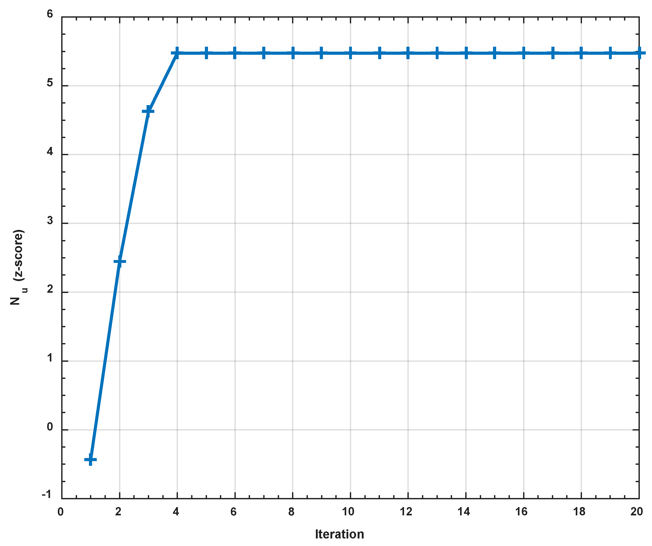
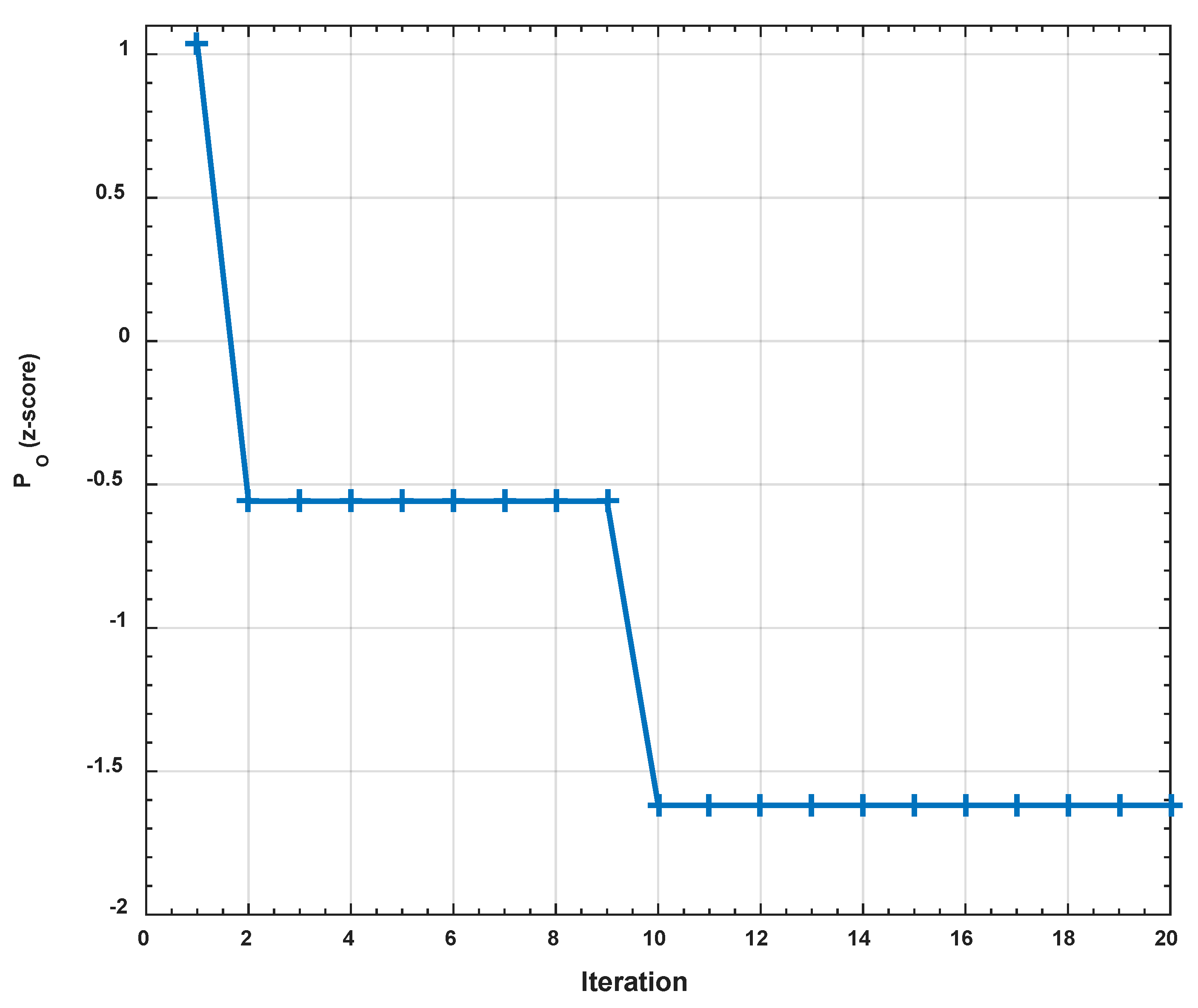
• Without going back to the numerical data, the proposed models were used with the PSO algorithm to find the optimal values of Po and Nu.
• The optimal values of Po and Nu are found when $\epsilon =1$ and $Kn=0.001$.
• The correlation coefficient of the models was greater than 0.95.
• The optimal values of the curves were determined when the curves became stable.

References

1. Liu, J.; Tai, Y.-C.; Pong, C.-M.H.-C. MEMS for pressure distribution studies of gaseous flows in microchannels. In Proceedings of the IEEE Micro Electro Mechanical Systems, Amsterdam, The Netherlands, 29 January–2 February 1995; p. 209. [Google Scholar]
2. Arkilic, E.B. Gaseous Flow in Micro-channels, Application of Microfabrication to Fluid Mechanics. AsmeFed 1994, 197, 57–66. [Google Scholar]
3. Ameel, T.A.; Wang, X.; Barron, R.F.; Warrington, R.O. Laminar forced convection in a circular tube with constant heat flux and slip flow. Microscale Thermophys. Eng. 1997, 1, 303–320. [Google Scholar]
4. Zade, A.Q.; Renksizbulut, M.; Friedman, J. Heat transfer characteristics of developing gaseous slip-flow in rectangular microchannels with variable physical properties. Int. J. Heat Fluid Flow 2011, 32, 117–127. [Google Scholar] [CrossRef]
5. Ghodoossi, L. Prediction of heat transfer characteristics in rectangular microchannels for slip flow regime and H1 boundary condition. Int. J. Therm. Sci. 2005, 44, 513–520. [Google Scholar] [CrossRef]
6. Hettiarachchi, H.M.; Golubovic, M.; Worek, W.M.; Minkowycz, W. Three-dimensional laminar slip-flow and heat transfer in a rectangular microchannel with constant wall temperature. Int. J. Heat Mass Transf. 2008, 51, 5088–5096. [Google Scholar] [CrossRef]
7. Yu, S.; Ameel, T.A. Slip-flow heat transfer in rectangular microchannels. Int. J. Heat Mass Transf. 2001, 44, 4225–4234. [Google Scholar] [CrossRef]
8. Renksizbulut, M.; Niazmand, H.; Tercan, G. Slip-flow and heat transfer in rectangular microchannels with constant wall temperature. Int. J. Therm. Sci. 2006, 45, 870–881. [Google Scholar] [CrossRef]
9. Tamayol, A.; Hooman, K. Slip-flow in microchannels of non-circular cross sections. J. Fluids Eng. 2011, 133, 091202. [Google Scholar] [CrossRef]
10. Hooman, K. A superposition approach to study slip-flow forced convection in straight microchannels of uniform but arbitrary cross-section. Int. J. Heat Mass Transf. 2008, 51, 3753–3762. [Google Scholar] [CrossRef] [Green Version]
11. Sadeghi, A.; Saidi, M.H. Viscous dissipation and rarefaction effects on laminar forced convection in microchannels. J. Heat Transf. 2010, 132, 072401. [Google Scholar] [CrossRef]
12. Yovanovich, M.; Khan, W.A. Compact Slip Flow Models for Gas Flows in Rectangular, Trapezoidal and Hexagonal Microchannels. In Proceedings of the ASME 2015 International Technical Conference and Exhibition on Packaging and Integration of Electronic and Photonic Microsystems, San Francisco, CA, USA, 6–9 July 2015. [Google Scholar]
13. Duan, Z.; Muzychka, Y. Slip flow in elliptic microchannels. Int. J. Therm. Sci. 2007, 46, 1104–1111. [Google Scholar] [CrossRef]
14. Duan, Z.; Muzychka, Y. Slip flow in non-circular microchannels. Microfluid. Nanofluid. 2007, 3, 473–484. [Google Scholar] [CrossRef] [Green Version]
15. Duan, Z.; Muzychka, Y. Slip flow in the hydrodynamic entrance region of circular and noncircular microchannels. J. Fluids Eng. 2010, 132, 011201. [Google Scholar] [CrossRef]
16. Yovanovich, M.M.; Khan, W.A. Friction and Heat Transfer in Liquid and Gas Flows in Micro-and Nanochannels. Adv. Heat Transf. 2015, 47, 203–307. [Google Scholar]
17. Ebert, W.; Sparrow, E.M. Slip flow in rectangular and annular ducts. J. Basic Eng. 1965, 87, 1018–1024. [Google Scholar] [CrossRef]
18. Baghani, M.; Sadeghi, A.; Baghani, M. Gaseous slip flow forced convection in microducts of arbitrary but constant cross section. Nanoscale Microscale Thermophys. Eng. 2014, 18, 354–372. [Google Scholar] [CrossRef]
19. Wang, C. Benchmark solutions for slip flow and H1 heat transfer in rectangular and equilateral triangular ducts. J. Heat Transf. 2013, 135, 021703. [Google Scholar] [CrossRef]
20. Beskok, A.; Karniadakis, G.E. Report: A model for flows in channels, pipes, and ducts at micro and nano scales. Microscale Thermophys. Eng. 1999, 3, 43–77. [Google Scholar]
21. Yovanovich, M.; Khan, W. Similarities of rarefied gas flows in elliptical and rectangular microducts. Int. J. Heat Mass Transf. 2016, 93, 629–636. [Google Scholar] [CrossRef]
22. Klášterka, H.; Vimmr, J.; Hajžman, M. Contribution to the gas flow and heat transfer modelling in microchannels. Appl. Comput. Mech. 2009, 12, 63–74. [Google Scholar]
23. Hamadneh, N.; Tilahun, S.; Sathasivam, S.; Choon, O.H. Prey-predator algorithm as a new optimization technique using in radial basis function neural networks. Res. J. Appl. Sci. 2013, 8, 383–387. [Google Scholar]
24. Rakhshandehroo, G.R.; Vaghefi, M.; Aghbolaghi, M.A. Forecasting groundwater level in Shiraz plain using artificial neural networks. Arab. J. Sci. Eng. 2012, 37, 1871–1883. [Google Scholar] [CrossRef]
25. Yeung, D.S.; Li, J.-C.; Ng, W.W.; Chan, P.P. MLPNN training via a multiobjective optimization of training error and stochastic sensitivity. IEEE Trans. Neural Netw. Learn. Syst. 2016, 27, 978–992. [Google Scholar] [CrossRef] [PubMed]
26. Mefoued, S. Assistance of knee movements using an actuated orthosis through subject’s intention based on MLPNN approximators. In Proceedings of the 2013 International Joint Conference on Neural Networks, Dallas, TX, USA, 4–9 August 2013; pp. 1–6. [Google Scholar]
27. Shi, Y.; Eberhart, R.C. Empirical study of particle swarm optimization. In Proceedings of the 1999 Congress on Evolutionary Computation, Washington, DC, USA, 6–9 July 1999; pp. 1945–1950. [Google Scholar]
28. Trelea, I.C. The particle swarm optimization algorithm: Convergence analysis and parameter selection. Inf. Process. Lett. 2003, 85, 317–325. [Google Scholar] [CrossRef]
29. Liu, X. Radial basis function neural network based on PSO with mutation operation to solve function approximation problem. In Proceedings of the International Conference in Swarm Intelligence, Brussels, Belgium, 8–10 September 2010; pp. 92–99. [Google Scholar]
30. Eberhart, R.; Kennedy, J. A new optimizer using particle swarm theory. In Proceedings of the Sixth International Symposium on Micro Machine and Human Science, Nagoya, Japan, 4–6 October 1995; pp. 39–43. [Google Scholar]
31. Shi, Y. Particle swarm optimization: Developments, applications and resources. In Proceedings of the 2001 Congress on Evolutionary Computation, Seoul, Korea, 27–30 May 2001; pp. 81–86. [Google Scholar]
32. Marinke, R.; Araujo, E.; Coelho, L.S.; Matiko, I. Particle swarm optimization (PSO) applied to fuzzy modeling in a thermal-vacuum system. In Proceedings of the Fifth International Conference on Hybrid Intelligent Systems, Rio de Janeiro, Brazil, 6–9 November 2005; p. 6. [Google Scholar]
33. Nenortaite, J.; Butleris, R. Application of particle swarm optimization algorithm to decision making model incorporating cluster analysis. In Proceedings of the 2008 Conference on Human System Interactions, Krakow, Poland, 25–27 May 2008; pp. 88–93. [Google Scholar]
34. Hamadneh, N.; Khan, W.A.; Sathasivam, S.; Ong, H.C. Design optimization of pin fin geometry using particle swarm optimization algorithm. PLoS ONE 2013, 8, e66080. [Google Scholar] [CrossRef] [PubMed]
35. Bai, Q. Analysis of particle swarm optimization algorithm. Comput. Inf. Sci. 2010, 3, 180. [Google Scholar] [CrossRef]
36. Morini, G.L.; Spiga, M.; Tartarini, P. The rarefaction effect on the friction factor of gas flow in microchannels. Superlattices Microstruct. 2004, 35, 587–599. [Google Scholar] [CrossRef]
37. Sadeghi, M.; Sadeghi, A.; Saidi, M.H. Gaseous slip flow mixed convection in vertical microducts of constant but arbitrary geometry. J. Thermophys. Heat Transf. 2014, 28, 771–784. [Google Scholar] [CrossRef]
38. Shah, R.; London, A. Laminar Flow Forced Convection in Ducts, Advances in Heat Transfer; Academic Press: New York, NY, USA, 1978. [Google Scholar]
Figure 1. Structure of a multilayer perceptron neural network (MLPNN).
Symmetry 11 00488 g001
Figure 2. Structure of the particle swarm optimization (PSO) algorithm.
Symmetry 11 00488 g002
Figure 3. Schematic diagram of rectangular microduct.
Symmetry 11 00488 g003
Figure 4. Best Validation Performance is 0.00020768 at iteration 187 of using MATLAB to generate the NN model of Nu.
Symmetry 11 00488 g004
Figure 5. Best Validation Performance is 0.00022112 at iteration 452 using MATLAB to generate the neural network (NN) model of Po.
Symmetry 11 00488 g005
Figure 6. Correlation coefficient and the regression of the NN model values of Nu and the desired values.
Symmetry 11 00488 g006
Figure 7. Correlation coefficient and the regression of the NN model values of Po and the desired values.
Symmetry 11 00488 g007
Figure 8. Best performance of the PSO algorithm in terms of Nu.
Symmetry 11 00488 g008
Figure 9. Best performance of the PSO algorithm in terms of Po.
Symmetry 11 00488 g009