Article

An m-Polar Fuzzy Hypergraph Model of Granular Computing

1
Department of Mathematics, University of the Punjab, New Campus, P.O. Box 54590, Lahore, Pakistan
2
Department of Mathematics, College of Science, Jazan University, New Campus, P.O. Box 2097, Jazan, Saudi Arabia
*
Author to whom correspondence should be addressed.
Symmetry 2019, 11(4), 483; https://doi.org/10.3390/sym11040483
Submission received: 12 March 2019 / Revised: 30 March 2019 / Accepted: 1 April 2019 / Published: 3 April 2019

Abstract

:
An m-polar fuzzy model plays a vital role in modeling of real-world problems that involve multi-attribute, multi-polar information and uncertainty. The m-polar fuzzy models give increasing precision and flexibility to the system as compared to the fuzzy and bipolar fuzzy models. An m-polar fuzzy set assigns the membership degree to an object belonging to [ 0 , 1 ] m describing the m distinct attributes of that element. Granular computing deals with representing and processing information in the form of information granules. These information granules are collections of elements combined together due to their similarity and functional/physical adjacency. In this paper, we illustrate the formation of granular structures using m-polar fuzzy hypergraphs and level hypergraphs. Further, we define m-polar fuzzy hierarchical quotient space structures. The mappings between the m-polar fuzzy hypergraphs depict the relationships among granules occurring at different levels. The consequences reveal that the representation of the partition of a universal set is more efficient through m-polar fuzzy hypergraphs as compared to crisp hypergraphs. We also present some examples and a real-world problem to signify the validity of our proposed model.

1. Introduction

Granular computing (GrC) is defined as an identification of techniques, methodologies, tools, and theories that yields the advantages of clusters, groups, or classes, i.e., the granules. The terminology was first introduced by Lin [1]. The fundamental concepts of GrC are utilized in various disciplines, including machine learning, rough set theory, cluster analysis, and artificial intelligence. Different models have been proposed to study the various issues occurring in GrC, including classification of the universe, illustration of granules, and the identification of relations among granules. For example, the procedure of problem solving through GrC can be considered as subdivisions of the problem at multiple levels, and these levels are linked together to construct a hierarchical space structure (HSS). Thus, this is a way of dealing with the formation of granules and the switching between different granularities. Here, the word “hierarchy” implies the methodology of hierarchical analysis in solving a problem and human activities [2]. To understand this methodology, let us consider an example of a national administration in which the complete nation is subdivided into various provinces. Further, we divide every province into various divisions, and so on. The human activities and problem solving involve the simplification of original complicated problem by ignoring some details rather than thinking about all points of the problem. This rationalized model is then further refined till the issue is completely solved. Thus, we resolve and interpret the complex problems from the weaker grain to the stronger one or from highest rank to lowest or from universal to particular, etc. This technique is called hierarchical problem solving. It is further acknowledged that the hierarchical strategy is the only technique that is used by humans to deal with complicated problems, and it enhances competency and efficiency. This strategy is also known as the multi-GrC.
Hypergraphs, as an extension of classical graphs, experience various properties that appear very effective and useful as the basis of different techniques in many fields, including problem solving, declustering, and databases [3]. The real-world problems that are represented and solved using hypergraphs have achieved very good impacts. The formation of hypergraphs is the same as that of granule structures, and the relations between the vertices and hyperedges of hypergraphs can depict the relationships of granules and objects. A hyperedge can contain n vertices representing n-ary relations and hence can provide more effective analysis and description of granules. Many researchers have used hypergraph methods to study the clustering of complex documentation by means of GrC and investigated the database techniques [4,5]. Chen et al. [6] proposed a model of GrC based on the crisp hypergraph. They related a crisp hypergraph to a set of granules and represented the hierarchical structures using series of hypergraphs. They proved a hypergraph model as a visual description of GrC.
Zadeh’s [7] fuzzy set (FS) has acquired greater attention by researchers in a wide range of scientific areas, including management sciences, robotics, decision theory, and many other disciplines. Zhang [8] generalized the idea of FSs to the concept of bipolar fuzzy sets (BFSs) whose membership degrees range over the interval [ 1 , 1 ] . An m-polar fuzzy set (m-PFS), as an extension of FS and BFS, was proposed by Chen et al. [9], and it proved that two-PFSs and BFSs are equivalent concepts in mathematics. An m-PFS corresponds to the existence of “multipolar information” because there are many real-world problems that take data or information from n agents ( n 2 ). For example, in the case of telecommunication safety, the exact membership degree lies in the interval [ 0 , 1 ] n ( n 7 × 10 9 ) as the distinct members are monitored at different times. Similarly, there are many problems that are based on n logic implication operators ( n 2 ), including rough measures, ordering results of magazines, fuzziness measures, etc.
To handle uncertainty in the representation of different objects or in the relationships between them, fuzzy graphs (FGs) were defined by Rosenfeld [10]. m-Polar fuzzy graphs and their interesting properties were discussed by Akram et al. [11] to deal with the network models possessing multi-attribute and multipolar data. As an extension of FGs, Kaufmann [12] defined fuzzy hypergraphs. Gong and Wang [13] investigated fuzzy classification by combining fuzzy hypergraphs with the fuzzy formal concept analysis and fuzzy information system. Although, many researchers have explored the construction of granular structures using hypergraphs in various fields, there are many graph theoretic problems that may contain uncertainty and vagueness. To overcome the problems of uncertainty in models of GrC, Wang and Gong [14] studied the construction of granular structures by means of fuzzy hypergraphs. They concluded that the representation of granules and partition is more efficient through the fuzzy hypergraphs. Novel applications and transversals of m-PF hypergraphs were defined by Akram and Sarwar [15,16]. Further, Akram and Shahzadi [17] studied various operations on m-PF hypergraphs. Akram and Luqman [18,19] introduced intuitionistic single-valued and bipolar neutrosophic hypergraphs. The basic purpose of this work is to develop an interpretation of granular structures using m-PF hypergraphs. In the proposed model, the vertex of the m-PF hypergraph denotes an object, and an m-PF hyperedge represents a granule. The “refinement” and “coarsening” operators are defined to switch the different granularities from coarser to finer and vice versa, respectively.
The rest of the paper is arranged as follows: In Section 2, some fundamental concepts of m-PF hypergraphs are reviewed. The uncertainty measures and information entropy of m-polar fuzzy hierarchical quotient space structure are discussed. An m-PFHQSS is developed based on the m-PF equivalence relation. In the next section, we construct an m-PF hypergraph model of GrC. The partition and covering of granules are defined in the same section. The method of bottom-up construction is explained by an algorithm. In Section 4, we construct a model of GrC using level hypergraphs based on the m-PF equivalence relation and explain the procedure of bottom-up construction through an example. Section 5 deals with some concluding remarks and future studies.

2. Fundamental Features of m -Polar Fuzzy Hypergraphs

In this section, we review some basic concepts from [9,11,15,16].
Definition 1.
An m-polar fuzzy set (m-PFS) M on a universal set Z is defined as a mapping M: Z [ 0 , 1 ] m . The membership degree of each element z Z is represented by M ( z ) = ( P 1 M ( z ) , P 2 M ( z ) , P 3 M ( z ) , …, P m M ( z ) ) , where P j M ( z ) : [ 0 , 1 ] m [ 0 , 1 ] is defined as the jth projection mapping.
Note that the mth power of [ 0 , 1 ] (i.e., [ 0 , 1 ] m ) is regarded as a partially-ordered set with the point-wise order ≤, where m is considered as an ordinal number ( m = n | n < m when m > 0 ) , ≤ is defined as z 1 z 2 if and only if P j ( z 1 ) P j ( z 2 ) , for every 1 j m . 0 = ( 0 , 0 , , 0 ) and 1 = ( 1 , 1 , , 1 ) are the smallest and largest values in [ 0 , 1 ] m , respectively.
Definition 2.
Let M be an m-PFS on Z. An m-polar fuzzy relation (m-PFR) N = ( P 1 N , P 2 N , P 3 N , …, P m N ) on M is a mapping N : M M such that N ( z 1 z 2 ) inf { M ( z 1 ) , M ( z 2 ) } , for all z 1 , z 2 Z , i.e., for each 1 j m , P j N ( z 1 z 2 ) inf { P j M ( z 1 ) , P j M ( z 2 ) } , where P j M ( z ) and P j N ( z 1 z 2 ) denote the jth membership degree of an element z Z and the pair z 1 z 2 , respectively.
Definition 3.
An m-polar fuzzy graph (m-PFG) on Z is defined as an ordered pair of functions G = ( C , D ) , where C : Z [ 0 , 1 ] m is an m-polar vertex set and D : Z × Z [ 0 , 1 ] m is an m-polar edge set of G such that D ( w z ) inf { C ( w ) , C ( z ) } , i.e., P j D ( w z ) inf { P j C ( w ) , P j C ( z ) } , for all w , z Z and 1 j m .
Definition 4.
An m-polar fuzzy hypergraph (m-PFHG) on a non-empty set Z is a pair H = ( A , B ) , where A = { M 1 , M 2 , …, M r } is a finite family of m-PFSs on Z and B is an m-PFR on m-PFSs M k such that:
  • B ( E k ) = B ( { z 1 , z 2 , , z l } ) inf { M k ( z 1 ) , M k ( z 2 ) , ⋯, M k ( z l ) } ,
  • k = 1 r s u p p ( M k ) = Z , for all M k A and for all z 1 , z 2 , , z l Z .
Definition 5.
Let H = ( A , B ) be an m-PFHG and τ [ 0 , 1 ] m . Then, the τ-cut level set of an m-PFS M is defined as,
M τ = { z | P j M ( z ) t j , 1 j m } , τ = ( t 1 , t 2 , , t m ) .
H τ = ( A τ , B τ ) is called a τ-cut level hypergraph of H, where A τ = i = 1 r M i τ .
For further concepts and applications, readers are referred to [20,21,22,23].

2.1. Uncertainty Measures of m-Polar Fuzzy Hierarchical Quotient Space Structure

The question of distinct membership degrees of the same object from different scholars has arisen because of various ways of thinking about the interpretation of different functions dealing with the same problem. To resolve this issue, FS was structurally defined by Zhang and Zhang [24], which was based on quotient space (QS) theory and the fuzzy equivalence relation (FER) [25]. This definition provides some new initiatives regarding membership degree, called a hierarchical quotient space structure (HQSS) of an FER. By following the same concept, we develop an HQSS of an m-polar FER.
Definition 6.
An m-polar fuzzy equivalence relation (PFER) on a non-empty finite set Z is called an m-PF similarity relation if it satisfies,
1. 
N ( z , z ) = ( P 1 N ( z , z ) , P 2 N ( z , z ) ,…, P m N ( z , z ) ) = ( 1 , 1 , , 1 ) , for all z Z ,
2. 
N ( u , w ) = ( P 1 N ( u , w ) , P 2 N ( u , w ) ,…, P m N ( u , w ) ) = ( P 1 N ( w , u ) , P 2 N ( w , u ) ,…, P m N ( w , u ) ) = N ( w , u ) , for all u , w Z .
Definition 7.
An m-PFER on a non-empty finite set Z is called an m-polar fuzzy equivalence relation (m-PFER) if it satisfies the conditions,
1. 
N ( z , z ) = ( P 1 N ( z , z ) , P 2 N ( z , z ) ,…, P m N ( z , z ) ) = ( 1 , 1 , , 1 ) , for all z Z ,
2. 
N ( u , w ) = ( P 1 N ( u , w ) , P 2 N ( u , w ) ,…, P m N ( u , w ) ) = ( P 1 N ( w , u ) , P 2 N ( w , u ) ,…, P m N ( w , u ) ) = N ( w , u ) , for all u , w Z ,
3. 
for all u , v , w Z , N ( u , w ) = sup v Z { min ( N ( u , v ) , N ( v , w ) ) } , i.e.,
P j N ( u , w ) = sup v Z { min ( P j N ( u , v ) , P j N ( v , w ) ) } , 1 j m .
Definition 8.
An m-polar fuzzy quotient space (m-PFQS) is denoted by a triplet ( Z , C ˜ , N ) , where Z is a finite domain, C ˜ represents the attributes of Z, and N represents the m-PF relationship between the objects of universe Z, which is called the structure of the domain.
Definition 9.
Let z i and z j be two objects in the universe Z. The similarity between z i , z j Z having the attribute c ˜ k is defined as:
N ( z i , z j ) = | c ˜ i k c ˜ j k | | c ˜ i k c ˜ j k | ,
where c ˜ i k represents that object z i possesses the attribute c ˜ k and c ˜ j k represents that object z j possesses the attribute c ˜ k .
Proposition 1.
Let N be an m-PFR on a finite domain Z and N τ = { ( x , w ) | P j N ( x , w ) t j , 1 j m } , τ = ( t 1 , t 2 , , t j ) [ 0 , 1 ] . Then, N τ is an ER on Z and is said to be the cut-equivalence relation of N.
Proposition 1 represents that N τ is a crisp relation, which is equivalence on Z, and its knowledge space is given as ξ N τ ( X ) = X / N τ .
The value domain of an ER N on Z is defined as D = { N ( w , y ) | w , y Z } such that:
P j Z ( w ) P j Z ( y ) P j N ( x , y ) > 0 , 1 j m .
Definition 10.
Let N be an m-PFER on a finite set Z and D be the value domain of N. The set given by ξ Z ( N ) = { Z / N τ | τ D } is called the m-polar fuzzy hierarchical quotient space structure (m-PFHQS) of N.
Example 1.
Let Z = { w 1 , w 2 , w 3 , w 4 , w 5 , w 6 } be a finite set of elements and N 1 be a four-PFER on Z; the relation matrix M ˜ N 1 corresponding to N 1 is given as follows:
M ˜ N 1 = ( 1 , 1 , 1 , 1 ) ( 0.4 , 0.4 , 0.5 , 0.5 ) ( 0.5 , 0.5 , 0.4 , 0.4 ) ( 0.5 , 0.5 , 0.4 , 0.4 ) ( 0.5 , 0.5 , 0.4 , 0.4 ) ( 0.5 , 0.5 , 0.4 , 0.4 ) ( 0.4 , 0.4 , 0.5 , 0.5 ) ( 1 , 1 , 1 , 1 ) ( 0.8 , 0.8 , 0.9 , 0.9 ) ( 0.8 , 0.8 , 0.6 , 0.6 ) ( 0.8 , 0.8 , 0.6 , 0.6 ) ( 0.6 , 0.6 , 0.5 , 0.5 ) ( 0.5 , 0.5 , 0.4 , 0.4 ) ( 0.8 , 0.8 , 0.9 , 0.9 ) ( 1 , 1 , 1 , 1 ) ( 0.6 , 0.6 , 0.7 , 0.7 ) ( 0.6 , 0.6 , 0.7 , 0.7 ) ( 0.6 , 0.6 , 0.5 , 0.5 ) ( 0.5 , 0.5 , 0.4 , 0.4 ) ( 0.8 , 0.8 , 0.6 , 0.6 ) ( 0.6 , 0.6 , 0.7 , 0.7 ) ( 1 , 1 , 1 , 1 ) ( 0.7 , 0.8 , 0.7 , 0.8 ) ( 0.6 , 0.6 , 0.5 , 0.5 ) ( 0.5 , 0.5 , 0.4 , 0.4 ) ( 0.8 , 0.8 , 0.6 , 0.6 ) ( 0.6 , 0.6 , 0.7 , 0.7 ) ( 0.7 , 0.8 , 0.7 , 0.8 ) ( 1 , 1 , 1 , 1 ) ( 0.6 , 0.6 , 0.5 , 0.5 ) ( 0.5 , 0.5 , 0.4 , 0.4 ) ( 0.6 , 0.6 , 0.5 , 0.5 ) ( 0.6 , 0.6 , 0.5 , 0.5 ) ( 0.6 , 0.6 , 0.5 , 0.5 ) ( 0.6 , 0.6 , 0.5 , 0.5 ) ( 1 , 1 , 1 , 1 ) .
Its corresponding m-PFHQSS is given as,
Z / N 1 τ 1 = Z / N 1 ( t 1 , t 2 , t 3 , t 4 ) = { { w 1 , w 2 , w 3 , w 4 , w 5 , w 6 } } , Z / N 1 τ 2 = Z / N 1 ( t 1 , t 2 , t 3 , t 4 ) = { { w 1 } , { w 2 , w 3 , w 4 , w 5 , w 6 } } , Z / N 1 τ 3 = Z / N 1 ( t 1 , t 2 , t 3 , t 4 ) = { { w 1 } , { w 2 , w 3 , w 4 , w 5 } , { w 6 } } , Z / N 1 τ 4 = Z / N 1 ( t 1 , t 2 , t 3 , t 4 ) = { { w 1 } , { w 2 , w 3 } , { w 4 , w 5 } , { w 6 } } , Z / N 1 τ 5 = Z / N 1 ( t 1 , t 2 , t 3 , t 4 ) = { { w 1 } , { w 2 , w 3 } , { w 4 } , { w 5 } , { w 6 } } , Z / N 1 τ 6 = Z / N 1 ( t 1 , t 2 , t 3 , t 4 ) = { { w 1 } , { w 2 } , { w 3 } , { w 4 } , { w 5 } , { w 6 } } ,
where:
0 < τ 1 = ( t 1 , t 2 , t 3 , t 4 ) 0.4 , 0.4 < τ 2 = ( t 1 , t 2 , t 3 , t 4 ) 0.5 , 0.5 < τ 3 = ( t 1 , t 2 , t 3 , t 4 ) 0.6 , 0.6 < τ 4 = ( t 1 , t 2 , t 3 , t 4 ) 0.7 , 0.7 < τ 5 = ( t 1 , t 2 , t 3 , t 4 ) 0.8 , 0.8 < τ 6 = ( t 1 , t 2 , t 3 , t 4 ) 1 .
Hence, a four-PFQSS is given as ξ Z ( N 1 ) = { Z / N τ 1 , Z / N τ 2 , Z / N τ 3 , Z / N τ 4 , Z / N τ 5 , Z / N τ 6 } and is shown in Figure 1.
It is worth noting that the same HQSS can be formed by different four-PFERs. For instance, the relation matrix M ˜ N 2 of four-PFER generates the same HQSS as given by M ˜ N 1 . The relation matrix M ˜ N 2 is given as,
M ˜ N 1 = ( 1 , 1 , 1 , 1 ) ( 0.2 , 0.2 , 0.5 , 0.5 ) ( 0.6 , 0.6 , 0.4 , 0.4 ) ( 0.6 , 0.6 , 0.4 , 0.4 ) ( 0.6 , 0.6 , 0.4 , 0.4 ) ( 0.6 , 0.6 , 0.4 , 0.4 ) ( 0.2 , 0.2 , 0.5 , 0.5 ) ( 1 , 1 , 1 , 1 ) ( 0.2 , 0.2 , 0.5 , 0.5 ) ( 0.2 , 0.2 , 0.5 , 0.5 ) ( 0.2 , 0.2 , 0.5 , 0.5 ) ( 0.2 , 0.2 , 0.5 , 0.5 ) ( 0.6 , 0.6 , 0.4 , 0.4 ) ( 0.2 , 0.2 , 0.5 , 0.5 ) ( 1 , 1 , 1 , 1 ) ( 0.7 , 0.7 , 0.7 , 0.7 ) ( 0.7 , 0.7 , 0.7 , 0.7 ) ( 0.7 , 0.7 , 0.7 , 0.7 ) ( 0.6 , 0.6 , 0.4 , 0.4 ) ( 0.2 , 0.2 , 0.5 , 0.5 ) ( 0.7 , 0.7 , 0.7 , 0.7 ) ( 1 , 1 , 1 , 1 ) ( 0.8 , 0.8 , 0.7 , 0.8 ) ( 0.6 , 0.6 , 0.5 , 0.5 ) ( 0.6 , 0.6 , 0.4 , 0.4 ) ( 0.2 , 0.2 , 0.5 , 0.5 ) ( 0.7 , 0.7 , 0.7 , 0.7 ) ( 0.8 , 0.8 , 0.7 , 0.8 ) ( 1 , 1 , 1 , 1 ) ( 0.6 , 0.6 , 0.5 , 0.5 ) ( 0.6 , 0.6 , 0.4 , 0.4 ) ( 0.2 , 0.2 , 0.5 , 0.5 ) ( 0.7 , 0.7 , 0.7 , 0.7 ) ( 0.6 , 0.6 , 0.5 , 0.5 ) ( 0.6 , 0.6 , 0.5 , 0.5 ) ( 1 , 1 , 1 , 1 ) .
Furthermore, assuming the number of blocks in every distinct layer of this HQSS, a pyramid model can also be constructed as shown in Figure 2.

2.2. Information Entropy of m-PFHQSS

Definition 11.
Let N be an m-PFER on Z. Let ξ Z ( N ) = { Z ( τ 1 ) , Z ( τ 2 ) , Z ( τ 3 ) , ⋯, Z ( τ j ) } be its corresponding HQSS, where τ i = ( t 1 i , t 2 i , , t m i ) , i = 1 , 2 ,⋯,j and Z ( τ j ) < Z ( τ j 1 ) < < Z ( τ 1 ) . Then, the partition sequence of ξ Z ( N ) is given as P ( ξ Z ( N ) ) = { P 1 , P 2 , P 3 , ⋯, P j } , where P i = | Z ( τ i ) | , i = 1 , 2 , , j , and | . | denotes the number of elements in a set.
Definition 12.
Let N be an m-PFER on Z. Let ξ Z ( N ) = { Z ( τ 1 ) , Z ( τ 2 ) , Z ( τ 3 ) , ⋯, Z ( τ j ) } be its corresponding HQSS, where τ i = ( t 1 i , t 2 i , , t m i ) , i = 1 , 2 ,⋯,j, and Z ( τ j ) < Z ( τ j 1 ) < < Z ( τ 1 ) , P ( ξ Z ( N ) ) = { P 1 , and P 2 , ⋯, P j } is the partition sequence of ξ Z ( N ) . Assume that Z ( τ i ) = { Z i 1 , Z i 2 , ⋯, Z i P i } . The information entropy E Z ( τ i ) is defined as E Z ( τ i ) = r = 1 P i | Z i r | | Z | l n | Z i r | | Z | .
Theorem 1.
Let N be an m-PFER on Z. Let ξ Z ( N ) = { Z ( τ 1 ) , Z ( τ 2 ) , Z ( τ 3 ) , ⋯, Z ( τ j ) } be its corresponding HQSS, where τ i = ( t 1 i , t 2 i ,⋯, t m i ) , i = 1 , 2 ,⋯,j, then the entropy sequence E ( ξ Z ( N ) ) = { E Z ( τ 1 ) , E Z ( τ 2 ) , ⋯, E Z ( τ j ) } increases monotonically and strictly.
Proof. 
The terminology of HQSS implies that Z ( τ j ) < Z ( τ j 1 ) < < Z ( τ 1 ) , i.e., Z ( τ j 1 ) is a quotient subspace of Z ( τ j ) . Suppose that Z ( τ i ) = { Z i 1 , Z i 2 , , Z i P i } and Z ( τ i 1 ) = { Z ( i 1 ) 1 , Z ( i 1 ) 2 , ⋯, Z ( i 1 ) P ( i 1 ) } , then every sub-block of Z ( τ i 1 ) is an amalgam of sub-blocks of Z ( τ i ) . WLOG, it is assumed that only one sub-block Z i 1 , j in Z ( τ i 1 ) is formed by the combination of two sub-blocks Z i r , Z i s in Z ( τ i ) , and all other remaining blocks are equal in both sequences. Thus,
E Z ( τ j 1 ) = r = 1 P i 1 | Z i 1 , r | | Z | ln | Z i 1 , r | | Z | = r = 1 P j 1 | Z i 1 , r | | Z | ln | Z i 1 , r | | Z | r = j + 1 P i 1 | Z i 1 , r | | Z | ln | Z i 1 , r | | Z | | Z i 1 , j | | Z | ln | Z i 1 , j | | Z | = r = 1 P j 1 | Z i , r | | Z | ln | Z i , r | | Z | r = j + 1 P i | Z i , r | | Z | ln | Z i , r | | Z | | Z i , r | + | Z i , s | | Z | ln | Z i , r | + | Z i , s | | Z | .
Since:
| Z i , r | + | Z i , s | | Z | ln | Z i , r | + | Z i , s | | Z | = | Z i , r | | Z | ln | Z i , r | + | Z i , s | | Z | + | Z i , s | | Z | ln | Z i , r | + | Z i , s | | Z | > | Z i , r | | Z | ln | Z i , r | | Z | + | Z i , s | | Z | ln | Z i , s | | Z | .
Therefore, we have:
E Z ( τ j 1 ) < r = 1 P j 1 | Z i , r | | Z | ln | Z i , r | | Z | r = j + 1 P i | Z i , r | | Z | ln | Z i , r | | Z | | Z i , r | | Z | ln | Z i , r | | Z | | Z i , s | | Z | ln | Z i , s | | Z | = E Z ( τ j ) , ( 2 j n ) .
Hence, E Z ( τ 1 ) < E Z ( τ 2 ) < E Z ( τ 2 ) < < E Z ( τ j ) . □
Definition 13.
Let Z = { s 1 , s 2 , s 3 , ⋯, s n } be a non-empty set of the universe, and let P d ( Z ) = { Z 1 , Z 2 , Z 3 , ⋯, Z d } be a partition space (PS) of Z, where | P d ( Z ) | = d , then P d ( Z ) is called the d-order partition space(d-OPS) on Z.
Definition 14.
Let Z be a finite non-empty universe, and let P d ( Z ) = { Z 1 , Z 2 , Z 3 , ⋯, Z d } be a d-OPS on Z. Let | Z 1 | = l 1 , | Z 2 | = l 2 , ⋯, | Z d | = l d , and the sequence { l 1 , l 2 , ⋯, l d } is arranged in increasing order, then we got a new sequence χ ( d ) = { l 1 , l 2 , ⋯, l d } , which is also increasing and called a sub-block sequence of  P d ( Z ) .
Note that two different d-OPSs on Z may possess the similar sub-block sequence χ ( d ) .
Definition 15.
Let Z be a finite non-empty universe, and let P d ( Z ) = { Z 1 , Z 2 , Z 3 , ⋯, Z d } be a partition space of Z. Suppose that χ 1 ( d ) = { l 1 , l 2 , ⋯, l d } is a sub-block sequence of P d ( Z ) , then the ω-displacement of χ 1 ( d ) is defined as an increasing sequence χ 2 ( d ) = { l 1 , l 2 , ⋯, l r + 1 , ⋯, l s 1 , ⋯, l d } , where r < s , l r + 1 < l s 1 .
An ω-displacement is obtained by subtracting one from some bigger term and adding one to some smaller element such that the sequence keeps its increasing property.
Theorem 2.
A single time ω-displacement χ 2 ( d ) , which is derived from χ 1 ( d ) , satisfies E ( χ 1 ( d ) ) < E ( χ 2 ( d ) ) .
Proof. 
Let χ 1 ( d ) = { l 1 , l 2 , ⋯, l d } and χ 2 ( d ) = { l 1 , l 2 , ⋯, l r + 1 , ⋯, l s 1 , ⋯, l d } , l 1 + l 2 + + l d = k , then we have:
E ( χ 2 ( t ) ) = j = 1 d l l k ln l l k + l r k ln l r k + l s k ln l s k l r + 1 k ln l r + 1 k l s 1 k ln l s 1 k .
Let g ( z ) = z k ln z k l z k ln l z k , where l = l r + l s and g ( z ) = 1 k ln l z z . Suppose that g ( z ) = 0 , then we obtain a solution, i.e., z = l 2 . Furthermore, g ( z ) = l k ( l z ) z < 0 , 0 z l 2 , and g ( z ) is increasing monotonically. Let z 1 = l r and z 2 = l r + 1 , l r + 1 < l s 1 , i.e., z 1 < z 2 l 2 = l r + l s 2 . Since g ( z ) is monotone, then g ( z 2 ) g ( z 1 ) > 0 . Thus,
l r k ln l r k + l s k ln l s k l r + 1 k ln l r + 1 k l s 1 k ln l s 1 k > 0 .
Hence,
E ( χ 2 ( d ) ) = j = 1 d l l k ln l l k + l r k ln l r k + l s k ln l s k l r + 1 k ln l r + 1 k l s 1 k ln l s 1 k > l r + 1 k ln l r + 1 k + l s 1 k ln l s 1 k > j = 1 t l l k ln l l k = E ( χ 1 ( d ) ) .
This completes the proof. □

3. An m -Polar Fuzzy Hypergraph Model of Granular Computing

A granule is defined as a collection of objects or elements having thhe same attributes or characteristics and can be treated as a single unit.
Definition 16.
An object space is defined as a system ( Z , N ) , where Z is a universe of objects or elements and N = { n 1 , n 2 , n 3 , ⋯, n k } , k = | Z | is a family of relations between the elements of Z. For r k , n r N , n r Z × Z × × Z , if ( z 1 , z 2 , ⋯, z r ) n r , then there exists an r-array relation n r on ( z 1 , z 2 , ⋯, z n ) .
A granule is affiliated with a particular level. The whole view of granules at every level can be taken as a complete description of a particular problem at that level of granularity [6]. An m-PFHG formed by the set of relations N and membership degrees Z ( w ) = P j Z ( w ) , 1 j m of objects in the space is considered as a specific level of the GrC model. All m-PF hyperedges in that m-PFHG can be regarded as the complete granule at that particular level.
Definition 17.
A partition of a set Z established on the basis of relations between objects is defined as a collection of non-empty subsets, which are pairwise disjoint and whose union is the whole of Z. These subsets that form the partition of Z are called blocks. Every partition of a finite set Z contains the finite number of blocks. Corresponding to the m-PFHG, the constraints of partition ψ = { E i | 1 i n } can be stated as follows,
  • each E i is non-empty,
  • for i j , E i E j = ,
  • { s u p p ( E i ) | 1 i n } = Z .
Definition 18.
A covering of a set Z is defined as a collection of non-empty subsets whose union is the whole of Z. The conditions for the covering c = { E i | 1 i n } of Z are stated as,
  • each E i is non-empty,
  • { s u p p ( E i ) | 1 i n } = Z .
The corresponding definitions in classical hypergraph theory are completely analogous to the above Definitions 17 and 18. In a crisp hypergraph, if the hyperedges E i and E j do not intersect each other, i.e., E i , E j E , and E i E j = , then these hyperedges form a partition of granules at this level. Furthermore, if E i , E j E , and E i E j , i.e., the hyperedges E i and E j intersect each other, then these hyperedges form a covering at this level.
Example 2.
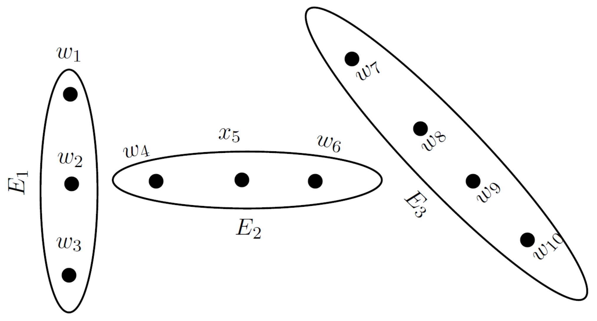
Let Z = { w 1 , w 2 , w 3 , w 4 , w 5 , w 6 , w 7 , w 8 , w 9 , w 10 } . The partition and covering of Z is given in Figure 3 and Figure 4, respectively.
A set-theoretic way to study the GrC model uses the following operators in an m-PFHG model.
Definition 19.
Let G 1 and G 2 be two granules in our model and the m-PF hyperedges, and E 1 , E 2 represent their external properties. The union of two granules G 1 G 2 is defined as a larger m-PF hyperedge that contains the vertices of both E 1 and E 2 . If w i G 1 G 2 , then the membership degree G 1 G 2 ( w i ) of w i in larger granule G 1 G 2 is defined as follows:
P j ( G 1 G 2 ) ( w i ) = max { P j ( E 1 ) ( w i ) , P j ( E 2 ) ( w i ) } , if w i E 1 and w i E 2 , P j ( E 1 ) ( w i ) , if w i E 1 and w i E 2 , P j ( E 2 ) ( w i ) , if w i E 2 and w i E 1 ,
1 j m .
Definition 20.
Let G 1 and G 2 be two granules in our model and the m-PF hyperedges, and E 1 , E 2 represent their external properties. The union of two granules G 1 G 2 is defined as a larger m-PF hyperedge that contains the vertices of both E 1 and E 2 . If w i G 1 G 2 , then the membership degree G 1 G 2 ( w i ) of w i in smaller granule G 1 G 2 is defined as follows:
P j ( G 1 G 2 ) ( w i ) = min { P j ( E 1 ) ( w i ) , P j ( E 2 ) ( w i ) } , if w i E 1 and w i E 2 , P j ( E 1 ) ( w i ) , if w i E 1 and w i E 2 , P j ( E 2 ) ( w i ) , if w i E 2 and w i E 1 ,
1 j m .
Definition 21.
Let G 1 and G 2 be two granules in our model and the m-PF hyperedges E 1 , E 2 represent their external properties. The difference between two granules G 1 G 2 is defined as a smaller m-PF hyperedge that contains those vertices belonging to E 1 , but not to E 2 .
Note that, if a vertex w i E 1 and w i E 2 , then:
P j ( E 1 ) ( w i ) > 0 and P j ( E 2 ) ( w i ) = 0 , 1 j m .
Definition 22.
A granule G 1 is said to be the sub-granule of G 2 , if each vertex w i of E 1 also belongs to E 2 , i.e., E 1 E 2 . In such a case, G 2 is called the super-granule of G 1 .
Note that, if E ( w i ) = { 0 , 1 } , then all the above described operators are reduced to the classical hypergraph theory of GrC.

Formation of Hierarchical Structures

We can interpret a problem at distinct levels of granularities. These granular structures at different levels produce a set of m-PFHGs. The upper set of these hypergraphs constructs a hierarchical structure at distinct levels. The relationships between granules are expressed by the lower level, which represents the problem as a concrete example of granularity. The relationships between granule sets are expressed by the higher level, which represents the problem as an abstract example of granularity. Thus, the single-level structures can be constructed and then can be subdivided into hierarchical structures using the relational mappings between different levels.
Definition 23.
Let H 1 = ( A 1 , B 1 ) and H 2 = ( A 2 , B 2 ) be two m-PFHGs. In a hierarchy structure, their level cuts are H τ 1 and H τ 2 , respectively, where τ = ( t 1 , t 2 , , t m ) . Let τ [ 0 , 1 ] and P j E i 1 t j , 1 j m , where E i 1 B 1 , then a mapping ϕ : H τ 1 H τ 2 from H τ 1 to H τ 2 maps the E τ i 1 in H τ 1 to a vertex w i 2 in H τ 2 . Furthermore, the mapping ϕ 1 : H τ 2 H τ 1 maps a vertex w i 2 in H τ 2 to the τ-cut of the m-PF hyperedge E τ i 1 in H τ i 1 . It can be denoted as ϕ ( E τ i 1 ) = w i 2 or ϕ 1 ( w i 2 ) = E τ i 1 , for 1 i n .
In an m-PFHG model, the mappings are used to describe the relations among different levels of granularities. At each distinct level, the problem is interpreted w.r.t the m-PF granularity of that level. The mapping associates the different descriptions of the same problem at distinct levels of granularities. There are two fundamental types to construct the method of hierarchical structures, the top-down construction procedure and the bottom-up construction procedure [26].
A formal discussion is provided to interpret an m-PFHG model in GrC, which is more compatible with human thinking. Zhang and Zhang [25] highlighted that one of the most important and acceptable characteristic of human intelligence is that the same problem can be viewed and analyzed at different granularities. Their claim is that the problem can not only be solved using various worlds of granularities, but also can be switched easily and quickly. Hence, the procedure of solving a problem can be considered as the calculations at different hierarchies within that model.
A multi-level granularity of the problem is represented by an m-PFHG model, which allows the problem solvers to decompose it into various minor problems and transform it into other granularities. The transformation of the problem in other granularities is performed by using two operators, i.e., zooming-in and zooming-out operators. The transformation from the weaker level to the finer level of granularity is done by the zoom-in operator, and the zoom-out operator deals with the shifting of the problem from coarser to finer granularity.
Definition 24.
Let H 1 = ( A 1 , B 1 ) and H 2 = ( A 2 , B 2 ) be two m-PFHGs, which are considered as two levels of hierarchical structures, and H 2 owns a coarser granularity than H 1 . Suppose H τ 1 = ( Z 1 , E τ 1 ) and H τ 2 = ( Z 2 , E τ 2 ) are the corresponding τ-level hypergraphs of H 1 and H 2 , respectively. Let e i 1 E τ 1 , z j 1 Z 1 , e j 2 E τ 2 , z l 2 , z m 2 Z 2 , and z l 2 , z m 2 e j 2 . If ϕ ( e i 1 ) = z l 2 , then n ( z j 1 , z m 2 ) is the relationship between z j 1 , and z m 2 is obtained by the characteristics of granules.
Definition 25.
Let the hyperedge ϕ 1 ( z l ) be a vertex at a new level and the relation between hyperedges in this level be the same as that of relationship between vertices at the previous level. This is called the zoom-in operator and transforms a weaker level to a stronger level. The function r ( z j 1 , z m 2 ) defines the relation between vertices of the original level, as well as the new level.
Let the vertex ϕ ( e i ) be a hyperedge at a new level, and the relation between vertices at this level is same as that of the relationship between hyperedges at the corresponding level. This is called the zoom-out operator and transforms a finer level to a coarser level.
By using these zoom-in and zoom-out operators, a problem can be viewed at multiple levels of granularities. These operations allow us to solve the problem more appropriately, and granularity can be switched easily at any level of problem solving.
In an m-PFHG model of GrC, the membership degrees of elements reflect the actual situation more efficiently, and a wide variety of complicated problems in uncertain and vague environments can be presented by means of m-PFHGs. The previous analysis concluded that this model of GrC generalizes the classical hypergraph model and fuzzy hypergraph model.
Definition 26
([6]). Let H 1 and H 2 be two crisp hypergraphs. Suppose that H 1 owns a finer m-PF granularity than H 2 . A mapping from H 1 to H 2 ψ : H 1 H 2 maps a hyperedge of H 1 to the vertex of H 2 , and the mapping ψ 1 : H 2 H 1 maps a vertex of H 2 to the hyperedge of H 1 .
The procedure of bottom-up construction for the level hypergraph model is illustrated in Algorithm 1.
Algorithm 1: The procedure of bottom-up construction for the level hypergraph model.
Step 1.
Determine an m-PFER matrix according to the actual circumstances.
Step 2.
For fixed τ [ 0 , 1 ] , obtain the corresponding HQSS.
Step 3.
Obtain the hyperedges through the HQSS.
Step 4.
Granules at the i-level are mapped to the ( i + 1 ) -level.
Step 5.
Calculate the m-polar fuzzy relationships between the vertices of the ( i + 1 ) -level, and determine the m-PFER matrix.
Step 6.
Determine the corresponding HQSS according to τ , which is fixed in Step 2.
Step 7.
Get the hyperedges at the ( i + 1 ) -level, and the ( i + 1 ) -level of the model is constructed.
Step 8.
Step 1–Step 5 are repeated until the whole universe is formulated to a single granule.
Definition 27.
Let N be an m-PFER on Z. A coarse-gained universe Z / N τ can be obtained by using m-PFER, where [ w i ] N τ = { w j Z | w i N w j } . This equivalence class [ w i ] N τ is considered as an hyperedge in the level hypergraph.
Definition 28.
Let H 1 = ( Z 1 , E 1 ) and H 2 = ( Z 2 , E 2 ) be level hypergraphs of m-PFHGs, and H 2 has weaker granularity than H 1 . Suppose that e i 1 , e j 2 E 1 and w i 2 , w j 2 Z 2 , i , j = 1 , 2 , , n . The zoom-in operator ω : H 2 H 1 is defined as ω ( w i 2 ) = e i 1 , e i 1 E 1 . The relations between the vertices of H 2 define the relationships among the hyperedges at the new level. The zoom-in operator of two levels is shown in Figure 5.
Remark 1.
For all Z 2 , Z 2 Z 2 , we have ω ( Z 2 ) = w i 2 Z 2 ω ( w i 2 ) and ω ( Z 2 ) = w j 2 Z 2 ω ( w j 2 ) .
Theorem 3.
Let H 1 = ( Z 1 , E 1 ) and H 2 = ( Z 2 , E 2 ) be two levels and ω : H 2 H 1 be the zoom-in operator. Then, for all Z 2 , Z 2 Z 2 , the zoom-in operator satisfies,
(i) 
ω maps the empty set to an empty set, i.e., ω ( ) = ,
(ii) 
ω ( Z 2 ) = E 1 ,
(iii) 
ω ( [ Z 2 ] c ) = [ ω ( Z 2 ) ] c ,
(iv) 
ω ( Z 2 Z 2 ) = ω ( Z 2 ) ω ( Z 2 ) ,
(v) 
ω ( Z 2 Z 2 ) = ω ( Z 2 ) ω ( Z 2 ) ,
(vi) 
Z 2 Z 2 if and only if ω ( Z 2 ) ω ( Z 2 ) .
Proof. 
(i) It is trivially satisfied that ω ( ) = .
(ii)
As we know that for all w i 2 Z 2 , we have ω ( Z 2 ) = w i 2 Z 2 ω ( w i 2 ) , since ω ( w i 2 ) = e i 1 , we have ω ( Z 2 ) = w i 2 Z 2 ω ( w i 2 ) = e i 1 E 1 e i 1 = E 1 .
(iii)
Let [ Z 2 ] c = Z 2 and [ Z 2 ] c = Z 2 , then it is obvious that Z 2 Z 2 = and Z 2 Z 2 = Z 2 . It follows from (ii) that ω ( Z 2 ) = E 1 , and we denote by W 1 that edge set of H 1 on which the vertex set Z 2 of H 2 is mapped under ω , i.e., ω ( Z 2 ) = W 1 . Then, ω ( [ Z 2 ] c ) = ω ( Z 2 ) = w i 2 Z 2 ω ( w i 2 ) = e i 1 W 1 e i 1 = Z 1 and [ ω ( Z 2 ) ] c = [ w j 2 Z 2 ω ( w j 2 ) ] c = [ e j 1 E 1 e j 1 ] c = ( E 1 ) c . Since the relationship between hyperedges at the new level is the same as that of relations among vertices at the original level, we have ( E 1 ) c = Z 1 . Hence, we conclude that ω ( [ Z 2 ] c ) = [ ω ( Z 2 ) ] c .
(iv)
Assume that Z 2 Z 2 = Z 2 ˜ , then for all w i 2 Z 2 ˜ implies that w i 2 Z 2 and w i 2 Z 2 . Further, we have ω ( Z 2 Z 2 ) = ω ( Z 2 ˜ ) = w i 2 Z 2 ˜ ω ( w i 2 ) = e i 1 E 1 ˜ ω ( e i 1 ) = E 1 ˜ .
ω ( Z 2 ) ω ( Z 2 ) = { w i 2 Z 2 ω ( w i 2 ) } { w j 2 Z 2 ω ( w j 2 ) } = e i 1 E 1 e i 1 e j 1 E 1 e j 1 = E 1 E 1 . Since the relationship between hyperedges at the new level is the same as that of relations among vertices at the original level, we have E 1 E 1 = E 1 ˜ . Hence, we conclude that ω ( Z 2 Z 2 ) = ω ( Z 2 ) ω ( Z 2 ) .
(v)
Assume that Z 2 Z 2 = Z 2 ¯ . Then, we have ω ( Z 2 Z 2 ) = ω ( Z 2 ¯ ) = w i 2 Z 2 ¯ ω ( w i 2 ) = e i 1 E 1 ¯ ω ( e i 1 ) = E 1 ¯ .
ω ( Z 2 ) ω ( Z 2 ) = { w i 2 Z 2 ω ( w i 2 ) } { w j 2 Z 2 ω ( w j 2 ) } = e i 1 E 1 e i 1 e j 1 E 1 e j 1 = E 1 E 1 . Since, the relationship between hyperedges at the new level is the same as that of the relations among the vertices at the original level, we have E 1 E 1 = E 1 ¯ . Hence, we conclude that ω ( Z 2 Z 2 ) = ω ( Z 2 ) ω ( Z 2 ) .
(vi)
First we show that Z 2 Z 2 implies that ω ( Z 2 ) ω ( Z 2 ) . Since Z 2 Z 2 , which implies that Z 2 Z 2 = Z 2 and ω ( Z 2 ) = w i 2 Z 2 ω ( w i 2 ) = e i 1 E 1 e i 1 = E 1 . Furthermore, ω ( Z 2 ) = w j 2 Z 2 ω ( w j 2 ) = e j 1 E 1 e j 1 = E 1 . Since the relationship between hyperedges at the new level is the same as that of relations among vertices at the original level, we have E 1 E 1 , i.e., ω ( Z 2 ) ω ( Z 2 ) . Hence, Z 2 Z 2 implies that ω ( Z 2 ) ω ( Z 2 ) .
We now prove that ω ( Z 2 ) ω ( Z 2 ) implies that Z 2 Z 2 . Suppose on the contrary that whenever ω ( Z 2 ) ω ( Z 2 ) , then there is at least one vertex w i 2 Z 2 , but w i 2 Z 2 , i.e., Z 2 Z 2 . Since ω ( w i 2 ) = e i 1 and the relationship between hyperedges at the new level is the same as that of relations among vertices at the original level, we have e i 1 E 1 , but e i 1 E 1 , i.e., E 1 E 1 , which is a contradiction to the supposition. Thus, we have that ω ( Z 2 ) ω ( Z 2 ) implies that Z 2 Z 2 . Hence, Z 2 Z 2 if and only if ω ( Z 2 ) ω ( Z 2 ) .
Definition 29.
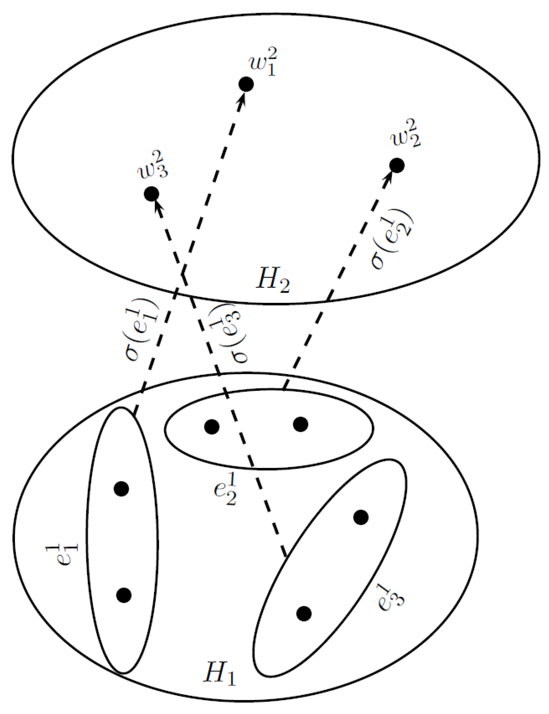
Let H 1 = ( Z 1 , E 1 ) and H 2 = ( Z 2 , E 2 ) be level hypergraphs of m-PFHGs, and H 2 has weaker granularity than H 1 . Suppose that e i 1 , e j 2 E 1 and w i 2 , w j 2 Z 2 , i , j = 1 , 2 , , n . The zoom-out operator σ : H 1 H 2 is defined as σ ( e i 1 ) = w i 2 , w i 2 Z 2 . The zoom-out operator of two levels is shown in Figure 6.
Theorem 4.
Let σ : H 1 H 2 be the zoom-out operator from H 1 = ( Z 1 , E 1 ) to H 2 = ( Z 2 , E 2 ) , and let E 1 E 1 . Then, the zoom-out operator σ satisfies the following properties,
(i) 
σ ( ) = ,
(ii) 
σ maps the set of hyperedges of H 1 onto the set of vertices of H 2 , i.e., σ ( E 1 ) = Z 2 ,
(iii) 
σ ( [ E 1 ] c ) = [ σ ( E 1 ) ] c .
Proof. 
(i) This part is trivially satisfied.
(ii)
According to the definition of σ , we have σ ( e i 1 ) = w i 2 . Since, the hyperedges define a partition of hypergraph, so we have E 1 = { e 1 1 , e 2 1 , e 3 1 , ⋯, e n 1 } = e i 1 E 1 e i 1 . Then,
σ ( E 1 ) = σ ( e i 1 E 1 e i 1 ) = e i 1 E 1 σ ( e i 1 ) = w i 2 Z 2 w i 2 = Z 2 .
(iii)
Assume that [ E 1 ] c = V 1 , then it is obvious that E 1 V 1 = and E 1 V 1 = E 1 . Suppose on the contrary, there exists at least one vertex w i 2 σ ( [ E 1 ] c ) , but w i 2 [ σ ( E 1 ) ] c . w i 2 σ ( [ E 1 ] c ) implies that w i 2 σ ( V 1 ) w i 2 e i 1 V 1 σ ( e i 1 ) w i 2 e i 1 E 1 E 1 σ ( e i 1 ) . Since w i 2 [ σ ( E 1 ) ] c w i 2 σ ( E 1 ) w i 2 e i 1 E 1 σ ( e i 1 ) , which is a contradiction to our assumption. Hence, σ ( [ E 1 ] c ) = [ σ ( E 1 ) ] c .
Definition 30.
Let H 1 = ( Z 1 , E 1 ) and H 2 = ( Z 2 , E 2 ) be two levels of m-PFHGs, and H 1 possesses a stronger granularity than H 2 . Let E 1 E 1 , then σ ^ ( E 1 ) = { e i 2 | e i 2 E 2 , κ ( e i 2 ) E 1 } is called the internal zoom-out operator. The operator σ ˇ ( E 1 ) = { e i 2 | e i 2 E 2 , κ ( e i 2 ) E 1 } is called the external zoom-out operator.
Example 3.
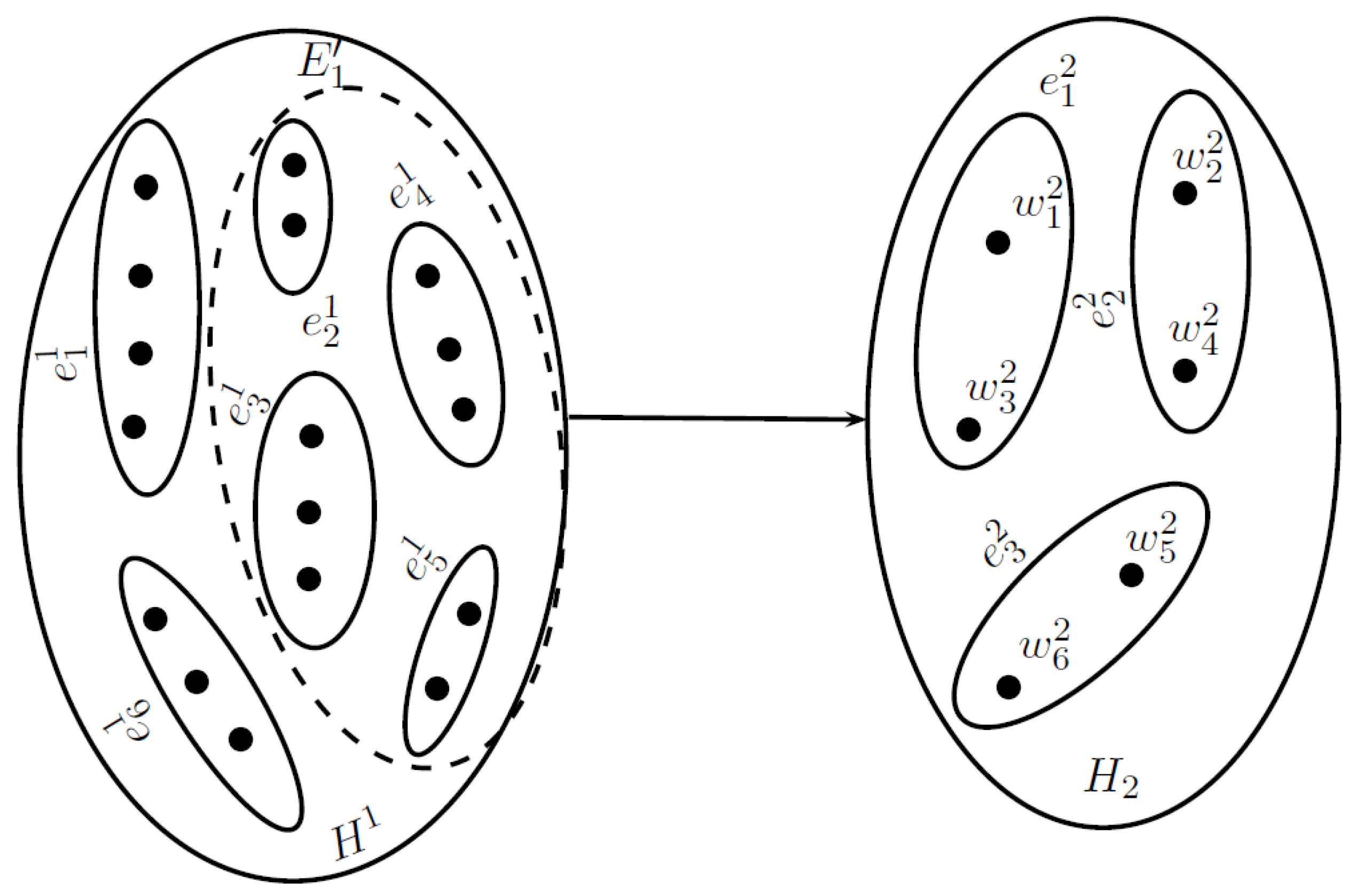
Let H 1 = ( Z 1 , E 1 ) and H 2 = ( Z 2 , E 2 ) be two levels of m-PFHGs, and H 1 possesses a stronger granularity than H 2 , where E 1 = { e 1 1 , e 2 1 , e 3 1 , e 4 1 , e 5 1 , e 6 1 } , and E 2 = { e 1 2 , e 2 2 , e 3 2 } . Furthermore, e 1 2 = { w 1 2 , w 3 2 } , e 2 2 = { w 2 2 , w 4 2 } , e 3 2 = { w 5 2 , w 6 2 } , as shown in Figure 7.
Let E 1 = { e 2 1 , e 3 1 , e 4 1 , e 5 1 } be the subset of hyperedges of H 1 , then we cannot zoom-out to H 2 directly; thus, by using the internal and external zoom-out operators, we have the following relations.
σ ^ ( { e 2 1 , e 3 1 , e 4 1 , e 5 1 } ) = { e 2 2 } ,
σ ˇ ( { e 2 1 , e 3 1 , e 4 1 , e 5 1 } ) = { e 1 2 , e 2 2 , e 3 2 } .

4. A Granular Computing Model of Web Searching Engines

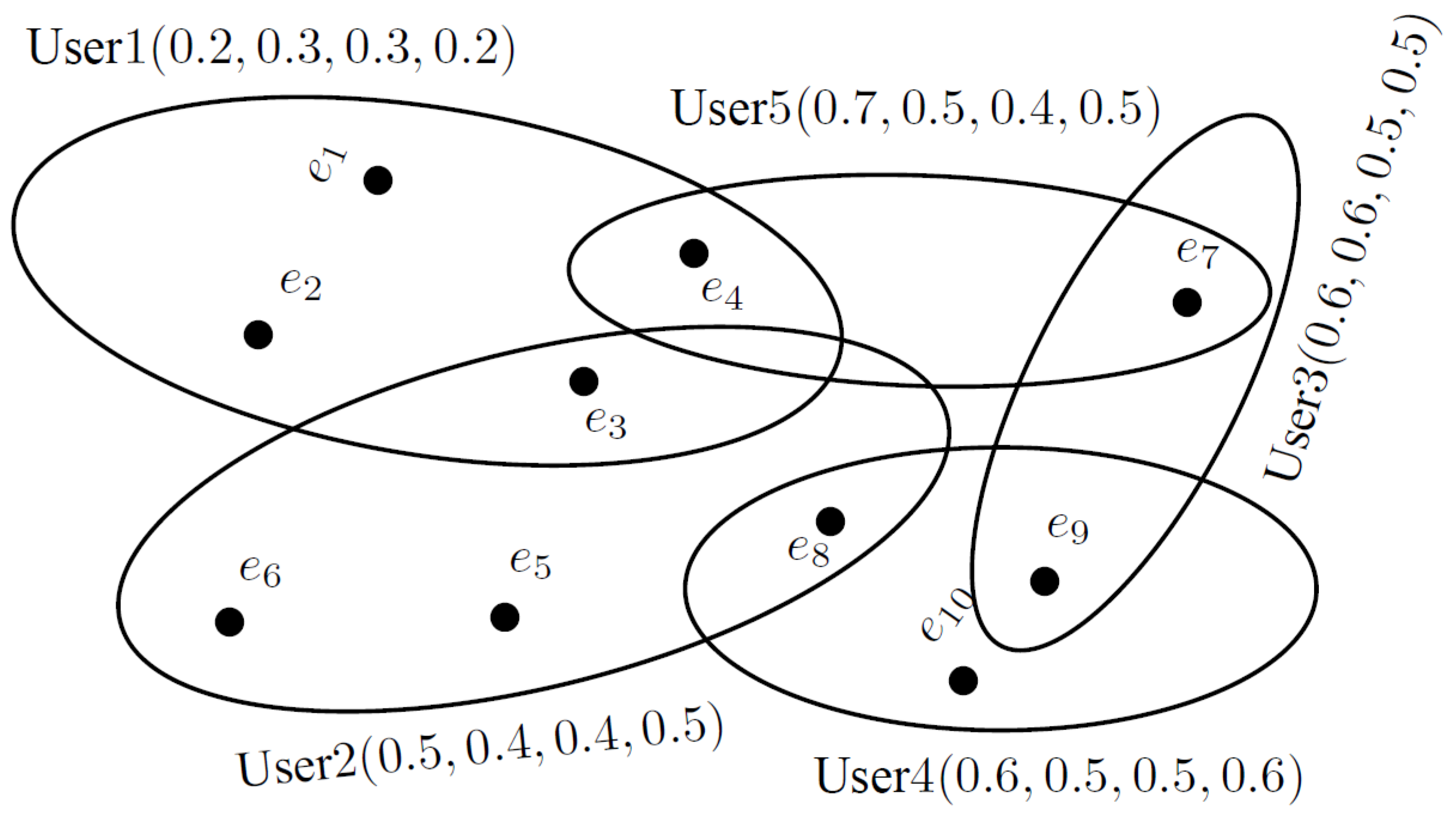
The most fertile way to direct a search on the Internet is through a search engine. A web search engine is defined as a system software that is designed to search for queries on the World Wide Web. A user may utilize a number of search engines to gather information, and similarly, various searchers may make an effective use of the same engine to fulfill their queries. In this section, we construct a GrC model of web searching engines based on four-PFHG. In a web searching hypernetwork, the vertices denote the various search engines. According to the relation set N, the vertices having some relationship are united together as a hyperedge, in which the search engines serve only one user. After assigning the membership degrees to that unit, a four-PF hyperedge is constructed, which is also considered as a granule. A four-PF hyperedge indicates a user that wants to gather some information, and the vertices in that hyperedge represent those search engines that provide relevant data to the user. Let us consider there are ten search engines, and the corresponding four-PFHG H = ( A , B ) is shown in Figure 8. Note that A = { e 1 , e 2 , e 3 , ⋯, e 10 } , and B = { U 1 , U 2 , U 3 , U 4 , U 5 } .
The incidence matrix of four-PFHG is given in Table 1.
An m-PFHG model of GrC illustrates a vague set having some membership degrees. In this model, there are five users that need the search engines to gather information. Note that the membership degrees of these engines are different for the users because whenever a user selects a search engine, he/she considers various factors or attributes. Hence, an m-PFHG in GrC is more meaningful and effective.
Let us suppose that each search engine possesses four attributes, which are core technology, scalability, content processing, and query functionality. The information table for various search engines having these attributes is given in Table 2.
The membership degrees of search engines reveal the percentage of attributes possessed by them, e.g., e 1 owns 70 % of core technology, 60 % scalability, and 50 % provide content processing, and the query functionality of this engine is 70 % . The four-PFER matrix describes the similarities between these search engines and is given as follows,
P ˜ N = 1 1 0.6 0.6 0.6 0.6 0.6 0.6 0.6 0 1 1 0.7 0.7 0.7 0.7 0.7 0.7 0.7 0 0.6 0.7 1 0.8 0.8 0.8 0.8 0.8 0.8 0 0.6 0.7 0.8 1 0.6 0.6 0.6 0.6 0.6 0.6 0.6 0.7 0.8 0.6 1 0.5 0.5 0.5 0.5 0 0.6 0.7 0.8 0.6 0.5 1 0.6 0.6 0.6 0 0.6 0.7 0.8 0.6 0.5 0.6 1 0.7 0.7 0.7 0.6 0.7 0.8 0.6 0.5 0.6 0.7 1 0.8 0.8 0.6 0.7 0.8 0.6 0.5 0.6 0.7 0.8 1 0.8 0 0 0 0.6 0 0 0.7 0.8 0.8 1 ,
where 1 = ( 1 , 1 , 1 , 1 ) , 0 = ( 0 , 0 , 0 , 0 ) , 0.5 = ( 0.5 , 0.5 , 0.5 , 0.5 ) , 0.6 = ( 0.6 , 0.6 , 0.6 , 0.6 ) , 0.7 = ( 0.7 , 0.7 , 0.7 , 0.7 ) , and 0.8 = ( 0.8 , 0.8 , 0.8 , 0.8 ) . Let τ = ( t 1 , t 2 , t 3 , t 4 ) = ( 0.7 , 0.7 , 0.7 , 0.7 ) , then its corresponding HQSS is given as follows,
Z / N τ = Z / N ( 0.7 , 0.7 , 0.7 , 0.7 ) = { { e 1 , e 2 } , { e 1 , e 2 , e 3 , e 4 , e 5 , e 6 , e 7 , e 8 , e 9 } , { e 2 , e 3 , e 5 } , { e 2 , e 3 , e 4 , e 5 , e 6 , e 7 , e 8 , e 9 } , { e 2 , e 3 , e 4 } , { e 2 , e 3 , e 6 } , { e 2 , e 3 , e 7 , e 8 , e 9 , e 10 } , { e 7 , e 8 , e 9 , e 10 } } .
Note that n 1 = n 5 = n 7 = n 10 = { } , n 2 = { ( e 1 , e 2 ) } , n 3 = { ( e 2 , e 3 , e 4 ) , ( e 2 , e 3 , e 5 ) , ( e 2 , e 3 , e 6 ) } , n 4 = { ( e 7 , e 8 , e 9 , e 10 ) } , n 6 = { e 2 , e 3 , e 7 , e 8 , e 9 , e 10 } , n 8 = { e 2 , e 3 , e 4 , e 5 , e 6 , e 7 , e 8 , e 9 } , n 9 = { e 1 , e 2 , e 3 , e 4 , e 5 , e 6 , e 7 , e 8 , e 9 } . Hence, a single level of the four-PFHG model is constructed and is shown in Figure 9.
Thus, we can obtain eight hyperedges E 1 = { e 1 , e 2 } , E 2 = { e 2 , e 3 , e 4 } , E 3 = { e 2 , e 3 , e 5 } , E 4 = { e 2 , e 3 , e 6 } , E 5 = { e 7 , e 8 , e 9 , e 10 } , E 6 = { e 2 , e 3 , e 7 , e 8 , e 9 , e 10 } , E 7 = { e 2 , e 3 , e 4 , e 5 , e 6 , e 7 , e 8 , e 9 } , E 8 = { e 1 , e 2 , e 3 , e 4 , e 5 , e 6 , e 7 , e 8 , e 9 } . The procedure of constructing this single-level model is explained in the following flowchart Figure 10.
We now illustrate the procedure of bottom-up construction through a concrete example and also explain our method through Algorithm 2.
Example 4.
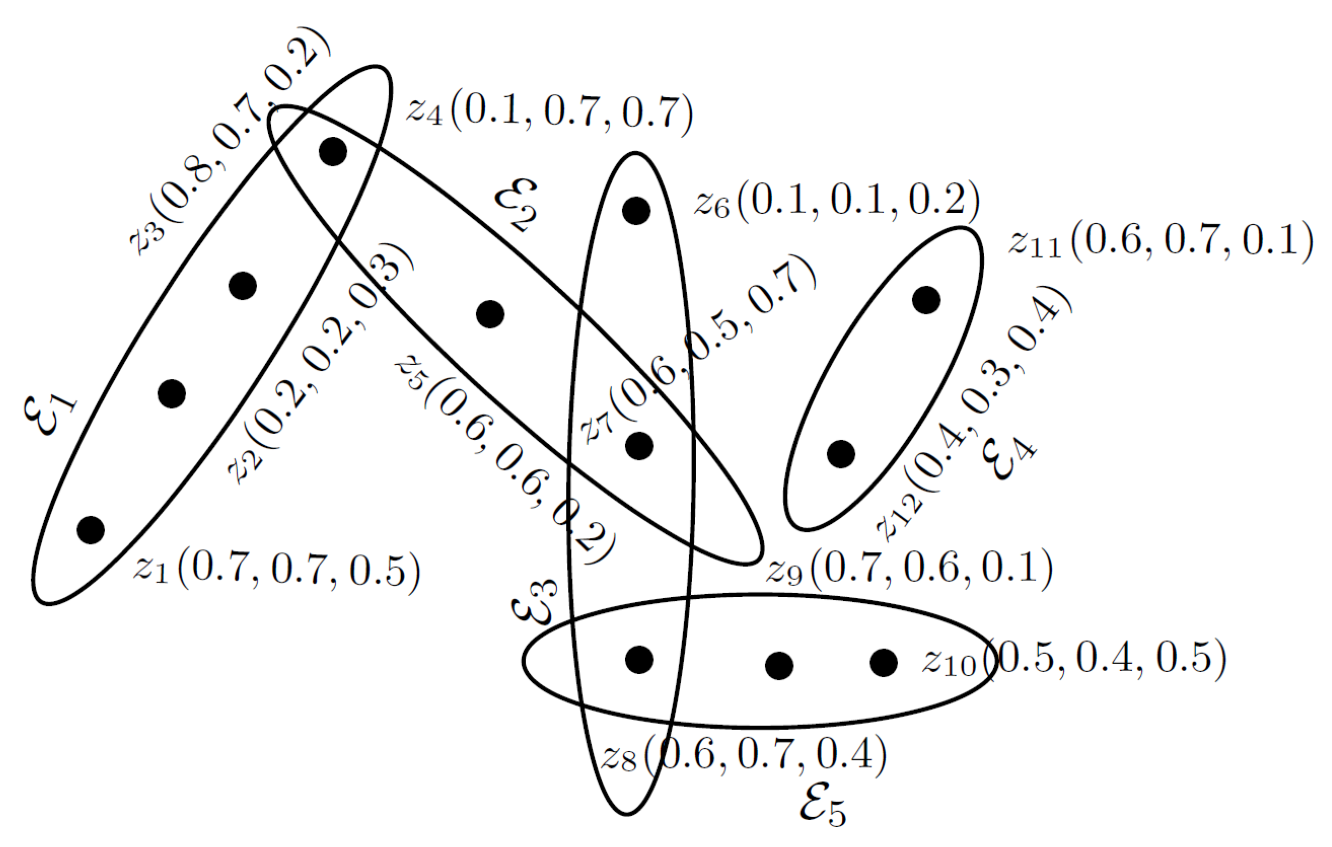
Let H = ( A , B ) be a three-PFHG as shown in Figure 11. Let Z = { z 1 , z 2 , z 3 , z 4 , z 5 , z 6 , z 7 , z 8 , z 9 , z 10 , z 11 , z 12 } , and B = { E 1 , E 2 , E 3 , E 4 , E 5 } .
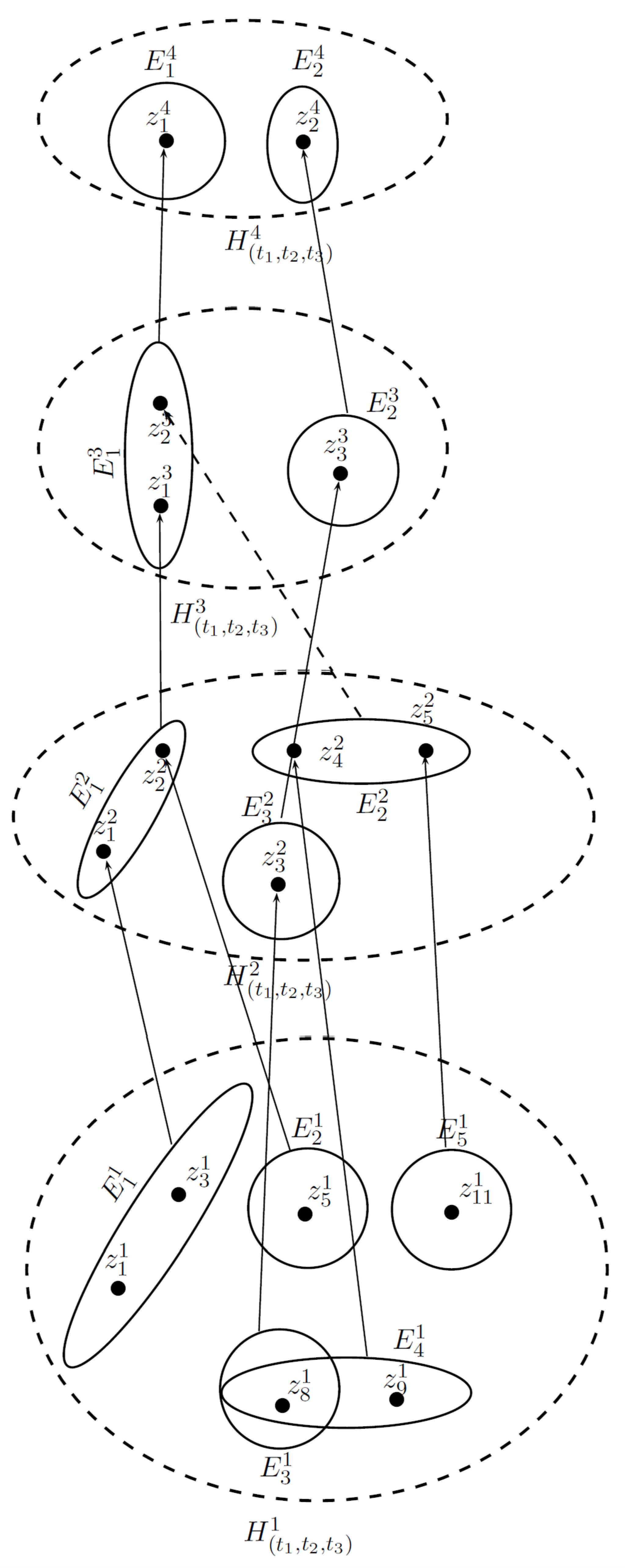
For t 1 = 0.5 , t 2 = 0.5 , and t 3 = 0.6 , the ( 0.5 , 0.5 , 0.6 ) -level hypergraph of H is given in Figure 12.
By considering the fixed t 1 , t 2 , t 3 and following Algorithm 2, the bottom-up construction of this model is given in Figure 13.
The possible method for the bottom-up construction is described in Algorithm 2.
Algorithm 2: Algorithm for the method of the bottom-up construction.
1 .  clc
2 . P j z i =input(‘ P j z i =’); T=input(‘ τ =’); q=1;
3 .     while q==1
4 .     [r, m]=size( P j z i );N=zeros(r, r);N=input(‘N=’); [ r 1 , r]=size(N); D=ones ( r 1 , m)+1;
5 .       for l=1: r 1
6 .            if N(l,:)==zeros(1, r)
7 .               D(l,:)=zeros(1, m);
8 .            else
9 .                 for k=1:r
10 .                      if N(l, k)==1
11 .                           for j=1:m
12 .                              D(l, j)=min(D(l, j), P j z i (k, j));
13 .                           end
14 .                      else
15 .                           s=0;
16 .                      end
17 .                 end
18 .            end
19 .       end
20 .       D
21 .       P j E i =input(‘ P j E i =’);
22 .       if size( P j E i )== [ r 1 , m]
23 .            if P j E i < =D
24 .                 if size(T)==[1, m]
25 .                    S=zeros( r 1 , r);s=zeros( r 1 , 1);
26 .                    for l=1: r 1
27 .                         for k=1:r
28 .                              if N(l, k)==1
29 .                                   if P j z i (k,:)>=T(1,:)
30 .                                     S(l, k)=1;
31 .                                     s(l, 1)=s(l, 1)+1;
32 .                                   else
33 .                                     S(l, k)=0;
34 .                                   end
35 .                              end
36 .                         end
37 .                    end
38 .                    S
39 .                    if s==ones( r 1 , 1)
40 .                      q=2;
41 .                    else
42 .                      P j z i = P j E i ;
43 .                    end
44 .                 else
45 .                    fprintf(‘error’)
46 .                 end
47 .            else
48 .              fprintf(‘error’)
49 .           end
50 .       else
51 .         fprintf(‘error’)
52 .       end
53 .     end

5. Conclusions

Granular computing (GrC) is a general framework to deal with granules, and it captures our ability to explore the real-world problems at different levels of granularity. It enables us to change these granularities during problem solving. The fundamental concepts of GrC are discussed in various environments, including cluster analysis, rough set theory, and artificial intelligence. The main objective of research in the field of GrC is to construct an effective computational model to deal with large amounts of information and knowledge. An m-PFS, as an extension of FS and BFS, is used to deal with multipolar information and multi-object network models. In this paper, we have used an m-PFHG model such that the benefits of m-PFSs and hypergraphs theory are combined to represent GrC. We have given a visual description of GrC and considered this model to examine the multi-polarity in GrC. After concise review of m-PFSs and m-PFHGs, we have applied these concepts in the formation of HQSSs. In this hypergraph model, we have obtained the granules as hyperedges from m-PFER, and the partition of the universe has been defined using these granules. Further, we have defined the zoom-in and zoom-out operators to give a description of the mappings between two hypergraphs. We have constructed a GrC model for web searching engines, which is based on multi-polar information. Moreover, we have discussed a concrete example to reveal the validity of our proposed model, and the procedure is represented through an algorithm. We aim to broaden our study to: ( 1 ) m-polar fuzzy directed hypergraphs, ( 2 ) fuzzy rough soft directed hypergraphs, ( 3 ) granular computing based on fuzzy rough and rough fuzzy hypergraphs, ( 4 ) hesitant m-polar fuzzy hypergraphs, and ( 5 ) the q-Rung picture fuzzy concept lattice.

Author Contributions

A.L., M.A. and A.N.A.K. conceived of the presented concept. A.L. and M.A. developed the theory and performed the computations. A.N.A.K. verified the analytical methods.

Acknowledgments

The authors are grateful to the Editor of the Journal and anonymous referees for their detailed and valuable comments.

Conflicts of Interest

The authors declare no conflict of interest.

References

  1. Lin, T.Y. Granular computing: From rough sets and neighborhood systems to information granulation and computing with words. In Proceedings of the European Congress on Intelligent Techniques and Soft Computing, Aachen, Germany, 8–12 September 1997. [Google Scholar]
  2. Zhang, L.; Zhang, B. Hierarchy and Multi-Granular Computing, Quotient Space Based Problem Solving; Tsinghua University Press: Beijing, China, 2014; pp. 45–103. [Google Scholar]
  3. Berge, C. Graphs and Hypergraphs; North-Holland Publishing Company: Amsterdam, The Netherlands, 1973. [Google Scholar]
  4. Liu, Q.; Jin, W.B.; Wu, S.Y.; Zhou, Y.H. Clustering research using dynamic modeling based on granular computing. In Proceedings of the IEEE International Conference on Granular Computing, Beijing, China, 25–27 July 2005; pp. 539–543. [Google Scholar]
  5. Wong, S.K.M.; Wu, D. Automated mining of granular database scheme. In Proceedings of the IEEE International Conference on Fuzzy Systems, St. Louis, MO, USA, 25–28 May 2002; pp. 690–694. [Google Scholar]
  6. Chen, G.; Zhong, N.; Yao, Y. A hypergraph model of granular computing. In Proceedings of the IEEE International Conference on Granular Computing, Hangzhou, China, 26–28 August 2008; pp. 130–135. [Google Scholar]
  7. Zadeh, L.A. Fuzzy sets. Inf. Control 1965, 8, 338–353. [Google Scholar] [CrossRef]
  8. Zhang, W.-R. Bipolar fuzzy sets and relations: A computational framework forcognitive modeling and multiagent decision analysis. In Proceedings of the First International Joint Conference of the North American Fuzzy Information Processing Society Biannual Conference, the Industrial Fuzzy Control and Intellige, San Antonio, TX, USA, 18–21 December 1994; pp. 305–309. [Google Scholar]
  9. Chen, J.; Li, S.; Ma, S.; Wang, Z. m-Polar fuzzy sets: An extension of bipolar fuzzy sets. Sci. World J. 2014, 2014, 416530. [Google Scholar] [CrossRef] [PubMed]
  10. Rosenfeld, A. Fuzzy graphs. In Fuzzy Sets and Their Applications to Cognitive and Decision Processes; Academic Press: New York, NY, USA, 1975; pp. 77–95. [Google Scholar]
  11. Akram, M. m-Polar fuzzy graphs. In Studies in Fuzziness and Soft Computing; Springer: Berlin, Germany, 2019; Volume 371, pp. 1–284. [Google Scholar]
  12. Kaufmann, A. Introduction a la Thiorie des Sous-Ensemble Flous; Masson: Paris, France, 1977. [Google Scholar]
  13. Gong, Z.; Wang, Q. On the connection of fuzzy hypergraph with fuzzy information system. J. Intell. Fuzzy Syst. 2017, 44, 1665–1676. [Google Scholar] [CrossRef]
  14. Wang, Q.; Gong, Z. An application of fuzzy hypergraphs and hypergraphs in granular computing. Inf. Sci. 2018, 429, 296–314. [Google Scholar] [CrossRef]
  15. Akram, M.; Sarwar, M. Novel applications of m-polar fuzzy hypergraphs. J. Intell. Fuzzy Syst. 2017, 32, 2747–2762. [Google Scholar] [CrossRef]
  16. Akram, M.; Sarwar, M. Transversals of m-polar fuzzy hypergraphs with applications. J. Intell. Fuzzy Syst. 2017, 33, 351–364. [Google Scholar] [CrossRef]
  17. Akram, M.; Shahzadi, G. Hypergraphs in m-polar fuzzy environment. Mathematics 2018, 6, 28. [Google Scholar] [CrossRef]
  18. Akram, M.; Luqman, A. Intuitionistic single-valued neutrosophic hypergraphs. Opsearch 2017, 54, 799–815. [Google Scholar] [CrossRef]
  19. Akram, M.; Luqman, A. Bipolar neutrosophic hypergraphs with applications. J. Intell. Fuzzy Syst. 2017, 33, 1699–1713. [Google Scholar] [CrossRef]
  20. Mordeson, J.N.; Nair, P.S. Fuzzy Graphs and Fuzzy Hypergraphs, 2nd ed.; Physica Verlag: Heidelberg, Germany, 2001. [Google Scholar]
  21. Parvathi, R.; Akram, M.; Thilagavathi, S. Intuitionistic fuzzy shortest hyperpath in a network. Inf. Process. Lett. 2013, 113, 599–603. [Google Scholar]
  22. Yang, J.; Wang, G.; Zhang, Q. Knowledge distance measure in multigranulation spaces of fuzzy equivalence relation. Inf. Sci. 2018, 448, 18–35. [Google Scholar] [CrossRef]
  23. Zhang, H.; Zhang, R.; Huang, H.; Wang, J. Some picture fuzzy Dombi Heronian mean operators with their application to multi-attribute decision-making. Symmetry 2018, 10, 593. [Google Scholar] [CrossRef]
  24. Zhang, L.; Zhang, B. The Theory and Applications of Problem Solving-Quotient Space Based Granular Computing; Tsinghua University Press: Beijing, China, 2007. [Google Scholar]
  25. Zhang, L.; Zhang, B. The structural analysis of fuzzy sets. J. Approx. Reason. 2005, 40, 92–108. [Google Scholar] [CrossRef]
  26. Yao, Y.Y. A partition model of granular computing. In Transactions on Rough Sets I. Lecture Notes in Computer Science; Peters, J.F., Skowron, A., Grzymala-Busse, J.W., Kostek, B., Swiniarski, R.W., Szczuka, M.S., Eds.; Springer: Berlin/Heidelberg, Germany, 2004. [Google Scholar]
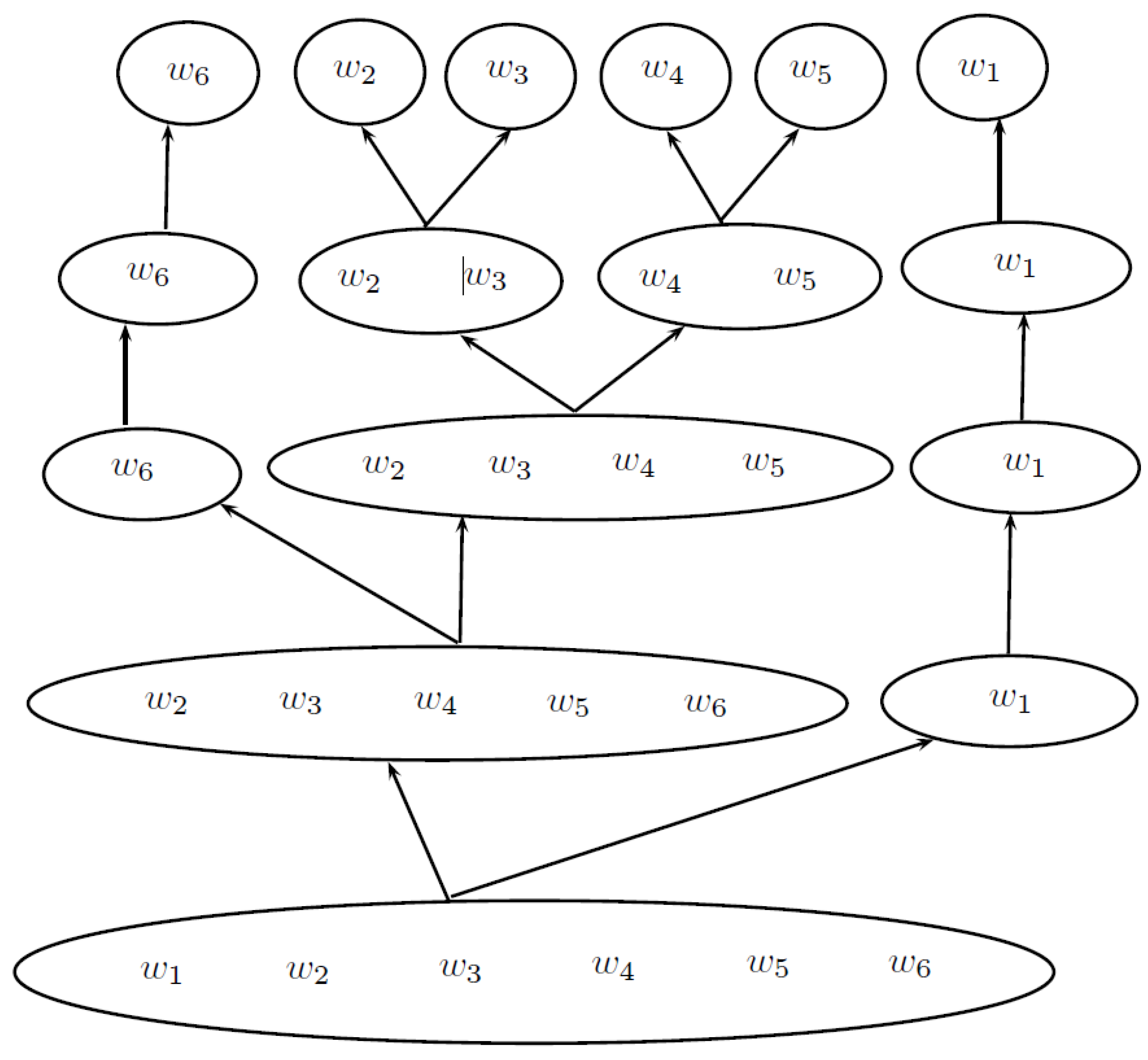
Figure 1. A four-polar fuzzy hierarchical quotient space structure.
Symmetry 11 00483 g001
Figure 2. Pyramid model of m-PFHQSS.
Symmetry 11 00483 g002
Figure 3. A partition of granules at a level.
Symmetry 11 00483 g003
Figure 4. A covering of granules at a level.
Symmetry 11 00483 g004
Figure 5. Zoom-in operator.
Symmetry 11 00483 g005
Figure 6. Zoom-out operator.
Symmetry 11 00483 g006
Figure 7. Internal and external zoom-out operators.
Symmetry 11 00483 g007
Figure 8. A four-PFHG representation of web searching.
Symmetry 11 00483 g008
Figure 9. A single-level model of four-PFHG.
Symmetry 11 00483 g009
Figure 10. Flowchart of the single-level model of m-PFHG.
Symmetry 11 00483 g010
Figure 11. A three-polar fuzzy hypergraph.
Symmetry 11 00483 g011
Figure 12. ( 0.5 , 0.5 , 0.6 ) -level hypergraph of H.
Symmetry 11 00483 g012
Figure 13. Bottom-up construction procedure.
Symmetry 11 00483 g013
Table 1. Incidence matrix.
A U 1 U 2 U 3 U 4 U 5
e 1 ( 0.2 , 0.3 , 0.3 , 0.2 ) ( 0 , 0 , 0 , 0 ) ( 0 , 0 , 0 , 0 ) ( 0 , 0 , 0 , 0 ) ( 0 , 0 , 0 , 0 )
e 2 ( 0.2 , 0.3 , 0.3 , 0.2 ) ( 0 , 0 , 0 , 0 ) ( 0 , 0 , 0 , 0 ) ( 0 , 0 , 0 , 0 ) ( 0 , 0 , 0 , 0 )
e 3 ( 0.2 , 0.3 , 0.3 , 0.2 ) ( 0.5 , 0.4 , 0.4 , 0.5 ) ( 0 , 0 , 0 , 0 ) ( 0 , 0 , 0 , 0 ) ( 0 , 0 , 0 , 0 )
e 4 ( 0.2 , 0.3 , 0.3 , 0.2 ) ( 0 , 0 , 0 , 0 ) ( 0 , 0 , 0 , 0 ) ( 0 , 0 , 0 , 0 ) ( 0.7 , 0.5 , 0.4 , 0.5 )
e 5 ( 0 , 0 , 0 , 0 ) ( 0.5 , 0.4 , 0.4 , 0.5 ) ( 0 , 0 , 0 , 0 ) ( 0 , 0 , 0 , 0 ) ( 0 , 0 , 0 , 0 )
e 6 ( 0 , 0 , 0 , 0 ) ( 0.5 , 0.4 , 0.4 , 0.5 ) ( 0 , 0 , 0 , 0 ) ( 0 , 0 , 0 , 0 ) ( 0 , 0 , 0 , 0 )
e 7 ( 0 , 0 , 0 , 0 ) ( 0 , 0 , 0 , 0 ) ( 0.6 , 0.6 , 0.5 , 0.5 ) ( 0 , 0 , 0 , 0 ) ( 0.7 , 0.5 , 0.4 , 0.5 )
e 8 ( 0 , 0 , 0 , 0 ) ( 0 , 0 , 0 , 0 ) ( 0 , 0 , 0 , 0 ) ( 0.6 , 0.5 , 0.5 , 0.6 ) ( 0 , 0 , 0 , 0 )
e 9 ( 0 , 0 , 0 , 0 ) ( 0 , 0 , 0 , 0 ) ( 0.6 , 0.6 , 0.5 , 0.5 ) ( 0.6 , 0.5 , 0.5 , 0.6 ) ( 0 , 0 , 0 , 0 )
e 10 ( 0 , 0 , 0 , 0 ) ( 0 , 0 , 0 , 0 ) ( 0 , 0 , 0 , 0 ) ( 0.6 , 0.5 , 0.5 , 0.6 ) ( 0 , 0 , 0 , 0 )
Table 2. The information table.
ACore TechnologyScalabilityContent ProcessingQuery Functionality
e 1 0.7 0.6 0.5 0.7
e 2 0.6 0.5 0.5 0.6
e 3 0.7 0.8 0.8 0.7
e 4 0.8 0.6 0.6 0.8
e 5 0.7 0.5 0.5 0.7
e 6 0.7 0.6 0.5 0.7
e 7 0.6 0.5 0.5 0.6
e 8 0.7 0.8 0.8 0.7
e 9 0.8 0.6 0.6 0.8
e 10 0.7 0.8 0.8 0.7