Article

Performance Analysis of Preemptive Priority Retrial Queueing System with Disaster under Working Breakdown Services

by
Sherif I. Ammar
1,2 and
Pakkirisamy Rajadurai
3,*
1
Department of Mathematics, College of Science, Taibah University, Madinah Munawwarah 414111, Saudi Arabia
2
Department of Mathematics, Menoufia University, Shebin El Koum 32511, Egypt
3
Department of Mathematics, Srinivasa Ramanujan Centre, SASTRA Deemed University, Kumbakonam 612001, India
*
Author to whom correspondence should be addressed.
Symmetry 2019, 11(3), 419; https://doi.org/10.3390/sym11030419
Submission received: 12 January 2019 / Revised: 25 February 2019 / Accepted: 4 March 2019 / Published: 21 March 2019

Abstract

:
In this investigation, a novel sort of retrial queueing system with working breakdown services is introduced. Two distinct kinds of customers are considered, which are priority and ordinary customers. The normal busy server may become inadequate due to catastrophes at any time which cause the major server to fail. At a failure moment, the major server is sent to be fixed and the server functions at a lower speed (called the working breakdown period) during the repair period. The probability generating functions (PGF) of the system size is found using the concepts of the supplementary variable technique (SVT). The impact of parameters in system performance measures and cost optimization are examined numerically.

1. Introduction

Every day we experience many queueing instances in which service is not prompt and customers need to wait to get service. The topic of retrial queues in queueing theory has been an interesting research topic in the last two decades. The retrial queues concept has received major efforts and attention from numerous researchers [1,2]. Such queueing models are employed in emerging applications in the performance analysis of an enormous scope of systems in telecommunications, data distributed networks, traffic management on high-speed networks and production engineering.
In retrial queueing literature, retrial queues with various sorts of customers have been widely investigated. The preemptive and non-preemptive priority concept plays a major role in priority discipline. In this regard, Choi and Park [3] provided a non-preemptive priority retrial queue through which customers enjoy non-preemptive priority as opposed to conventional customers. For an extensive examination of priority queueing models, the reader may refer to Wu and Lian [4], Gao [5] and Peng [6]. Priority retrial queues are utilized in many genuine implementations such as manufacturing systems, real-time systems and operating systems.
In the past, queueing models with different service rates were studied by several authors. The initiative of these models almost caused a change to the service rate depending on the situation of the system, such as queues in a random environment, queues with breakdown, working breakdown, models with vacations and working vacations. In 2002, Servi and Finn [7] presented an M/M/1 queueing system with working vacations. The M/M/1/WV queue to an M/G/1/WV queue was continued by Wu and Takagi [8]. Further, Tien Van Do [9] developed a model in M/M/1/WV with retrial concept. A short survey note on working vacation queueing models was written by Chandrasekaran et al. [10]. Authors like Arivudainambi et al. [11], Gao et al. [12], Rajadurai et al. [13], Gao and Liu [14], Zhang and Liu [15] analyzed the concepts of single server retrial queueing systems with working vacations.
In 2012, Kalidass and Ramanath [16] presented the idea of working breakdowns in M/M/1 queues, i.e., the system may face failure caused by disasters any time when the normal busy server is in service and the system ought to be ready with an alternate (standby) server in preparedness for possible prime server failures. The alternate server provides service to customers while the major server is repaired. The rate of service for the alternate server is diverse from (lower than) that of the major server. At the moment of the repair completion, the major server comes back to the system and is accessible again. Therefore, the working breakdown service is a progressively sensible repair policy for unreliable queueing systems. Recently, Kim and Lee [17] studied a model M/G/1 queueing system with disasters and working breakdown services. Utilizing the matrix geometric method, Ma et al. [18] obtained the stationary distribution of an M/M/1 queue with multiple vacations and working breakdowns. Recently, Deepa and Kalidass [19], Jiang and Liu [20], Liu and Song [21] and Rajadurai [22] developed a model disaster with working breakdowns.
Motivated by this factor, a new sort of M/G/1 preemptive priority retrial queue with disasters under working breakdown services is introduced in this work. During the working breakdown period, the server acts at a slow rate of service. The outcomes of this model are very helpful to decision-makers for developing management policies. The novelty of this work presents a generalization of priority retrial queueing models in the presence of working breakdown services. The result of these queueing models has convincing applications in Wireless Sensor Networks (WSNs), which are utilized in diverse applications to detect and transmit information to the localized node with energy effectiveness, thereby enlarging the network’s lifespan, namely the “Priority in Node Medium Access Control” (PRIN MAC) protocol that realizes quality of service (QoS) in terms of consuming the least energy to enlarge the lifetime of the network [23].
This investigation considers a general comparison of other systems on retrial queues in the sense that we have combined different characteristics together covering (i) priority arrival, (ii) disasters, (iii) breakdowns, (iv) working breakdown services and (v) repair whilst evolving the system for retrial queues.

2. Mathematical Model Description

We investigated a M/G/1 priority retrial queue with disasters under working breakdown services (priority policy of M/G/1/WB). The basic assumption of this model is described as follows:
  • The arrival process: Two sorts of customers were entered into the system: priority customers and regular customers. Priority customers have preemptive priorities over regular customers in relation to the service time of an occupied server. We supposed that both sorts of customers came as per three independent Poisson processes outgoing from the system with rates δ and λ, respectively.
  • The retrial process: We supposed that there was no waiting capacity and consequently an arriving priority customer saw the server free and the customer started the service directly. By the time the priority customer arrived, the server presented service for a priority customer or working breakdowns. A priority customer that arrived later would leave the system instantly wanting service. However, since the orderly occupied server was working with a regular customer, the arriving priority customer would obstruct the service of the regular customer as the server would directly start providing service to the priority customer.
  • We supposed that while an ordinary customer was preempted by a priority customer, the ordinary customer, who was solely being served before the service of the priority customer began, would wait in the service region for the residual service to finish. If an arriving ordinary customer discovered the server was occupied or was on working breakdown, the arrivals entered a pool of blocked customers, called an orbit, in accordance with FIFO discipline. This meant that only one customer at the head of the orbit queue was allowed to be served by the server. Then, measured from the instant the server became free, a potential priority customer, a regular customer and a retry customer competed to the entire server. Inter-retrial times are arbitrarily distributed R ( t ) with the Laplace Stieltijes Transform (LST) R ( ϑ ) . The retrial ordinary customer wanted to try to abandon the service if the first external customer or the average customer arrived first. In this case, the retrial ordinary customer returned to its location in the retrial queue.
  • The regular service process: Whenever a new primary (priority) customer or retry customer arrived at the server in idle state, then the server immediately started normal service for the arrivals. The service time of priority customers followed a general distribution denoted by the random variable Sp with distribution function S p ( t ) , having LST S p * ( ϑ ) and the first and second moments denoted as β p ( 1 ) and β p ( 2 ) . The service time of ordinary customers followed a general distribution denoted by the random variable Sb with distribution function S b ( t ) having LST S b * ( ϑ ) , and the first and second moments denoted as β b ( 1 )   and   β b ( 2 ) .
  • The working breakdown process: The system had the potential to become deficient by disasters at any time when the regular occupied server was in task with exponentially appropriated with a rate of α. The event of disasters forced all present ordinary customers out of the system and caused the primary server to fail. At a failure moment, the major server was sent to the reform, and the reform period started immediately. The repair time followed an exponential distribution with the rate of γ. We supposed that the repaired server was as good as a new server. Yet, disaster occurred in the regular working server or when the orbit became vacuous, after which the server left for a working breakdown. Through the duration of the working breakdown, the replacement server worked at a minimal service rate for the arriving customers (μw < μ). When the repair was completed, if there were customers in the orbit, the server changed to the normal working level. Alternatively, the server started another working breakdown period. Throughout the working breakdown periods (lower speed services), the service time pursued a general random variable Sw with distribution function S w ( t ) and LST S w * ( ϑ ) .
    We supposed that inter-arrival times, retrial times, service times and working breakdown times were disjointed and independent of one another.
  • Throughout the rest of the paper, we denote by F ¯ ( x ) = 1 F ( x ) the tail of distribution function F(x). We also denote F * ( s ) = 0 e s x d F ( x ) , to be the LST of F(x) and F ~ ( s ) = 0 e s x F ( x ) d x , to be the Laplace transform of F(x). Ee assume the notation F ¯ * ( s ) = 1 F * ( s ) s .

Practical Application of the Suggested Model

The proposed model has potential practical applications in the region of computer processing systems. In a computer processing system, if an arriving message (the customer) found that the processor (server) is complete, the messages would be incidentally put away in a retrial buffer (orbit) limited space to be served some time later (retrial time) according to FCFS. The working mail server might be influenced by a virus (breakdown) and the system may back off (working breakdown) the performance of the computer system. Therefore, the major mail server would be immediately sent for repair. The PC system may have the capacity to perform different errands, yet at a significantly slower rate (lower service speed). On the off chance that the processor is accessible, it would show that it is not currently chipping away at an errand and afterward a message would be prepared. If the processor is inaccessible, the messages would be briefly put away in a support section to be served some time later (retrial time) according to FCFS. This sort of working breakdown discipline is a decent estimation of a computer processing system.

3. Steady State Analysis of the System

For an M/G/1 priority retrial queue with disasters under working breakdowns (priority policy of M/G/1/WB), we constructed the steady state difference-differential equations based on the supplementary variable technique (SVT).

3.1. Steady State Probabilities and Notations

We defined the following notations:
  • N ( t ) the number of customers in the orbit at time t,
  • X ( t ) the state of the server at time t.
In addition, let ξ 1 0 ( t ) ,   ξ 2 0 ( t ) ,   ξ 3 0 ( t ) ,   ξ 4 0 ( t ) , be the elapsed times for retrial, service of priority and ordinary customers and working breakdowns, respectively, at time t.
Assume that A 1 ( 0 ) = 0 ,   A 1 ( ) = 1 ,   A 2 ( 0 ) = 0 ,   A 2 ( ) = 1 ,   A 4 ( 0 ) = 0 ,   A 4 ( ) = 1 are continuous at x = 0 and A 3 ( 0 ) = 0 , A 3 ( ) = 1 are continuous at y = 0.
Then the functions θ ( x ) ; μ p ( x ) ;   μ b ( y ) ;   μ w ( x ) . are the hazard rates for retrial, regular service for priority customers, ordinary customers and lower rate service, respectively.
i . e . ,   θ ( x ) d x = d A 1 ( x ) 1 A 1 ( x ) ; μ p ( x ) d x = d A 2 ( x ) 1 A 2 ( x ) ; μ b ( y ) d y = d A 3 ( y ) 1 A 3 ( y ) ; μ w ( x ) d x = d A 4 ( x ) 1 A 4 ( x ) .
Further, in the bivariate Markov process { X ( t ) , N ( t ) , t 0 } , X(t) denotes the server state (0, 1, 2, 3, 4, 5) depending on whether the server is free, busy for priority customers, ordinary customers and working breakdowns.
The steady state probabilities and limiting probability densities are defined as follows:
P 0 ( t ) = P { C ( t ) = 0 ,   N ( t ) = 0 } P i , n ( x ) d x = lim t P { C ( t ) = i , N ( t ) = n ,   x < ξ i 0 ( t ) x + d x } ,   for   t 0 ,   x 0   and   n 0 .   ( i = 1 , 2 , 4 , 5 ) P 3 , n ( x , y ) d x d y = lim t P { C ( t ) = 3 , N ( t ) = n ,   x < ξ 2 0 ( t ) x + d x ,   y < S b 0 ( t ) y + d y } ,   for   t 0 ,   x 0 ,   y 0 ,   n 0 .

3.2. Ergodicity Condition of the Model

We dissected the ergodicity of the embedded Markov chain at departure or vacation epochs. Let {tn; n = 1, 2, …} be the sequence of epochs at which either a normal service for priority/ordinary or a lower service completion occurs. The sequence of random vectors Z n = { X ( t n + ) ,   N ( t n + ) } forms an embedded Markov chain in the retrial queueing system. It follows from Appendix A that { Z n ;   n N } is ergodic if and only if ρ < A 1 * ( λ + δ ) , where ρ = ( A 1 * ( λ + δ ) + λ A ¯ 1 * ( λ + δ ) ) ( B A 3 * ( α ) + S ( 1 ) ) + δ λ A ¯ 1 * ( λ + δ ) β p ( 1 ) .

3.3. Steady State Equations

By the method of the SVT, we obtain the following system of equations:
( λ + δ + γ ) P 0 = γ P 0 +   0 P 2 , 0 ( x ) μ p ( x ) d x + 0 P 3 , 0 ( y ) μ b ( y ) d y + 0 P 5 , 0 ( x ) μ v ( x ) d x + α 0 P 4 , n ( y ) d y
d P 1 , n ( x ) d x + ( λ + δ + θ ( x ) ) P 1 , n ( x ) = 0 ,   n 1
d P 1 , 0 ( x ) d x + ( λ + θ ( x ) ) P 1 , 0 ( x ) = 0 ,   n = 0 ,
d P 2 , n ( x ) d x + ( λ + μ p ( x ) ) P 2 , n ( x ) = λ P 2 , n 1 ( x ) ,   n 1
P 3 , 0 ( x , y ) x + ( λ + μ p ( x ) ) P 3 , 0 ( x , y ) = 0 ,   n = 0 ,
P 3 , n ( x , y ) x + ( λ + μ p ( x ) ) P 3 , n ( x , y ) = λ P 3 , n 1 ( x , y ) ,   n 1 .
d P 4 , 0 ( y ) d y + ( λ + δ + α + μ b ( y ) ) P 4 , 0 ( y ) = 0 P 3 , 0 ( x , y ) μ p ( x ) d x ,   n = 0 .
d P 4 , n ( y ) d y + ( λ + δ + α + μ b ( y ) ) P 4 , n ( y ) = λ P 4 , n 1 ( y ) + 0 P 3 , n ( x , y ) μ p ( x ) d x ,   n 1
d P 5 , 0 ( x ) d x + ( λ + γ + μ w ( x ) ) P 5 , 0 ( x ) = 0 ,   n = 0 ,
d P 5 , n ( x ) d x + ( λ + γ + μ w ( x ) ) P 5 , n ( x ) = λ P 5 , n 1 ( x ) ,   n 1 .
The steady state boundary conditions at x = 0 and y = 0 are:
P 1 , n ( 0 ) = 0 P 2 , n ( x ) μ p ( x ) d x + 0 P 4 , n ( y ) μ b ( y ) d x + 0 P 5 , n ( x ) μ w ( x ) d x ,   n 1
P 2 , n ( 0 ) = δ 0 P 1 , n ( x ) d x ,   n 1
P 3 , n ( 0 , y ) = δ ( P 4 , n ( y ) ) ,   n 0
P 4 , 0 ( 0 ) = ( 0 P 1 , 1 ( x ) θ ( x ) d x + γ 0 P 5 , 0 ( x ) d x ) ,   n = 0
P 4 , n ( 0 ) = ( 0 P 1 , n + 1 ( x ) θ ( x ) d x + λ 0 P 1 , n ( x ) d x + γ 0 P 5 , n ( x ) d x ) ,   n 1
P 5 , n ( 0 ) = { ( λ + δ ) P 0 , n = 0 . 0 , n 1 .
The normalizing condition is:
P 0 + n = 1 0 P 1 , n ( x ) d x + n = 0 ( 0 P 2 , n ( x ) d x + 0 0 P 3 , n ( x , y ) d x d y + 0 P 4 , n ( y ) d y + 0 P 5 , n ( x ) d x ) = 1 .

3.4. Computation of the Steady State Solution

To analyze the developed queueing model, we make use of the SVT and the PGF method. We define the generating functions for |z| ≤ 1, as follows:
P 1 ( x , z ) = n = 1 P 1 , n ( x ) z n ;   P 1 ( 0 , z ) = n = 1 P 1 , n ( 0 ) z n ;   P 2 ( x , z ) = n = 0 P 2 , n ( x ) z n ;   P 2 ( 0 , z ) = n = 0 P 2 , n ( 0 ) z n ;   P 3 ( x , y , z ) = n = 0 P 3 , n ( x , y ) z n ;   P 3 ( 0 , y , z ) = n = 0 P 3 , n ( 0 , y ) z n ;   P 4 ( y , z ) = n = 0 P 4 , n ( y ) z n ; P 4 ( 0 , z ) = n = 0 P 4 , n ( 0 ) z n   ;   P 5 ( x , z ) = n = 0 P 5 , n ( x ) z n ;   P 5 ( 0 , z ) = n = 0 P 5 , n ( 0 ) z n ;
Theorem 1.
Based on the stability condition ρ < A 1 * ( λ + δ ) , the partial probability generating functions for server states are given by:
P 1 ( 0 , z ) = z ( λ + δ ) P 0 { W ( z ) ( A 3 * ( C ( z ) ) + S ( z ) ) + ( A 4 * ( D ( z ) ) 1 ) } { z ( A 1 * ( λ + δ ) + λ z A ¯ 1 * ( λ + δ ) ) ( A 3 * ( C ( z ) ) + S ( z ) ) z δ A ¯ 1 * ( λ + δ ) A 2 * ( B ( z ) ) }
P 2 ( 0 , z ) = z δ ( λ + δ ) A ¯ 1 * ( λ + δ ) P 0 { W ( z ) ( A 3 * ( C ( z ) ) + S ( z ) ) + ( A 4 * ( D ( z ) ) 1 ) } { z ( A 1 * ( λ + δ ) + λ z A ¯ 1 * ( λ + δ ) ) ( A 3 * ( C ( z ) ) + S ( z ) ) z δ A ¯ 1 * ( λ + δ ) A 2 * ( B ( z ) ) }
P 3 ( 0 , z ) = δ × P 4 ( 0 , z ) ( 1 A ¯ 3 * ( C ( z ) ) C ( z ) )
P 4 ( 0 , z ) = ( λ + δ ) P 0 { ( A 4 * ( D ( z ) ) 1 ) ( A 1 * ( λ + δ ) + λ z A ¯ 1 * ( λ + δ ) ) + z W ( z ) ( 1 δ A ¯ 1 * ( λ + δ ) ) } { z ( A 1 * ( λ + δ ) + λ z A ¯ 1 * ( λ + δ ) ) ( A 3 * ( C ( z ) ) + S ( z ) ) z δ A ¯ 1 * ( λ + δ ) A 2 * ( B ( z ) ) }
P 5 ( 0 , z ) = ( λ + δ ) P 0
where W ( z ) = γ ( 1 A 4 * ( D ( z ) ) ) D ( z ) ; S ( z ) = α ( 1 A 3 * ( C ( z ) ) ) C ( z ) ; A ¯ 2 * ( B ( z ) ) = ( 1 A 2 * ( B ( z ) ) B ( z ) ) ; A ¯ 3 * ( C ( z ) ) = ( 1 A 3 * ( C ( z ) ) C ( z ) ) ; B ( z ) = λ ( 1 z ) , C ( z ) = ( α + A p ( z ) + δ ( 1 A 2 * ( B ( z ) ) ) )   a n d   D ( z ) = ( γ + λ ( 1 z ) ) .
Proof. 
From Equations (2)–(16) multiplied by zn and Taking summation over n, (n = 0, 1, 2, …),
P 1 ( x , z ) x + ( λ + δ + θ ( x ) ) P 1 ( x , z ) = 0  
P 2 ( x , z ) x + ( λ ( 1 z ) + μ p ( x ) ) P 2 ( x , z ) = 0
P 3 ( x , y , z ) x + ( λ ( 1 z ) + μ p ( x ) ) P 3 ( x , y , z ) = 0
P 4 ( y , z ) y + ( λ ( 1 z ) + δ + α + μ b ( y ) ) P 4 ( y , z ) = 0 P 3 ( x , y , z ) μ p ( x ) d x
P 5 ( x , z ) x + ( λ ( 1 z ) + γ + μ w ( x ) ) P 5 ( x , z ) = 0 .
P 1 ( 0 , z ) = 0 P 2 ( x , z ) μ p ( x ) d x + 0 P 4 ( y , z ) μ b ( y ) d y + 0 P 5 ( x , z ) μ w ( x ) d x + α 0 P 4 ( y , z ) d y ( λ + δ ) P 0
P 2 ( 0 , z ) = δ 0 P 1 ( x , z ) d x
P 3 ( 0 , y , z ) = δ P 4 ( y , z )
P 4 ( 0 , z ) = 1 z 0 P 1 ( x , z ) θ ( x ) d x + λ 0 P 1 ( x , z ) d x + γ 0 P 5 ( x , z ) d x
P 5 ( 0 , z ) = ( λ + δ ) P 0 .
Solving the partial differential Equations (23)–(27), it follows that:
P 1 ( x , z ) = P 1 ( 0 , z ) [ 1 A 1 ( x ) ] e ( λ + δ ) x
P 2 ( x , z ) = P 2 ( 0 , z ) [ 1 A 2 ( x ) ] e B ( z ) x ,
P 3 ( x , y , z ) = P 3 ( 0 , y , z ) [ 1 A 2 ( x ) ] e B ( z ) x ,
P 4 ( y , z ) = P 4 ( 0 , z ) [ 1 A 3 ( y ) ] e C ( z ) y ,
P 5 ( x , z ) = P 5 ( 0 , z ) [ 1 A 4 ( x ) ] e D ( z ) x ,
where B ( z ) = λ ( 1 z ) , C ( z ) = ( α + A p ( z ) + δ ( 1 A 2 * ( B ( z ) ) ) )   a n d   D ( z ) = ( γ + λ ( 1 z ) )   .
Inserting Equation (33) in (29), we obtain:
P 2 ( 0 , z ) = δ P 1 ( 0 , z ) A 1 * ( λ + δ )
where A ¯ 1 * ( λ + δ ) = ( 1 A 1 * ( λ + δ ) λ + δ ) .
Using (36) in (30), we obtain:
P 3 ( 0 , y , z ) = δ × P 4 ( 0 , z ) ( 1 A 3 ( y ) ) e C ( y )
Inserting Equations (33) and (37) in Equation (31), we obtain:
P 4 ( 0 , z ) = P 1 ( 0 , z ) z ( A 1 * ( λ + δ ) + λ z A ¯ 1 * ( λ + δ ) ) + ( λ + δ ) P 0 W ( z )
where W ( z ) = γ ( 1 A 4 * ( D ( z ) ) ) D ( z ) ; A ¯ 2 * ( B ( z ) ) = ( 1 A 2 * ( B ( z ) ) B ( z ) ) ; A ¯ 3 * ( C ( z ) ) = ( 1 A 3 * ( C ( z ) ) C ( z ) ) ; .
Using (33)–(40) in (28), we obtain:
P 1 ( 0 , z ) =   P 2 ( 0 , z ) A 2 * ( B ( z ) ) + P 4 ( 0 , z ) ( A 3 * ( C ( z ) ) + S ( z ) ) + P 5 ( 0 , z ) A 4 * ( D ( z ) ) ( λ + δ ) P 0
where S ( z ) = α ( 1 A 3 * ( C ( z ) ) ) C ( z ) ; .
Using (38)–(40) in (41), we obtain:
{ z ( A 1 * ( λ + δ ) + λ z A ¯ 1 * ( λ + δ ) ) ( A 3 * ( C ( z ) ) + S ( z ) ) z δ A ¯ 1 * ( λ + δ ) A 2 * ( B ( z ) ) } P 1 ( 0 , z ) = z ( λ + δ ) P 0 { W ( z ) ( A 3 * ( C ( z ) ) + S ( z ) ) + ( A 4 * ( D ( z ) ) 1 ) }
From the above equation, we know that the key element for obtaining P ( 0 , z ) is to find the zeros of f ( z ) = { z ( A 1 * ( λ + δ ) + λ z A ¯ 1 * ( λ + δ ) ) ( A 3 * ( C ( z ) ) + S ( z ) ) z δ A ¯ 1 * ( λ + δ ) A 2 * ( B ( z ) ) } = 0 in the range 0 < z < 1 for the equation f ( z ) = 0 . (from [11]).
Using Equations (38)–(41) after making some manipulations, we obtain:
P 1 ( 0 , z ) = z ( λ + δ ) P 0 { W ( z ) ( A 3 * ( C ( z ) ) + S ( z ) ) + ( A 4 * ( D ( z ) ) 1 ) } { z ( A 1 * ( λ + δ ) + λ z A ¯ 1 * ( λ + δ ) ) ( A 3 * ( C ( z ) ) + S ( z ) ) z δ A ¯ 1 * ( λ + δ ) A 2 * ( B ( z ) ) }
P 2 ( 0 , z ) = z δ ( λ + δ ) A ¯ 1 * ( λ + δ ) P 0 { W ( z ) ( A 3 * ( C ( z ) ) + S ( z ) ) + ( A 4 * ( D ( z ) ) 1 ) } { z ( A 1 * ( λ + δ ) + λ z A ¯ 1 * ( λ + δ ) ) ( A 3 * ( C ( z ) ) + S ( z ) ) z δ A ¯ 1 * ( λ + δ ) A 2 * ( B ( z ) ) }
P 3 ( 0 , z ) = δ × P 4 ( 0 , z ) ( 1 A ¯ 3 * ( C ( z ) ) C ( z ) )
P 4 ( 0 , z ) = ( λ + δ ) P 0 { ( A 4 * ( D ( z ) ) 1 ) ( A 1 * ( λ + δ ) + λ z A ¯ 1 * ( λ + δ ) ) + z W ( z ) ( 1 δ A ¯ 1 * ( λ + δ ) ) } { z ( A 1 * ( λ + δ ) + λ z A ¯ 1 * ( λ + δ ) ) ( A 3 * ( C ( z ) ) + S ( z ) ) z δ A ¯ 1 * ( λ + δ ) A 2 * ( B ( z ) ) }
P 5 ( 0 , z ) = ( λ + δ ) P 0
where W ( z ) = γ ( 1 A 4 * ( D ( z ) ) ) D ( z ) ; S ( z ) = α ( 1 A 3 * ( C ( z ) ) ) C ( z ) ; A ¯ 2 * ( B ( z ) ) = ( 1 A 2 * ( B ( z ) ) B ( z ) ) ; A ¯ 3 * ( C ( z ) ) = ( 1 A 3 * ( C ( z ) ) C ( z ) ) ; B ( z ) = λ ( 1 z ) , C ( z ) = ( α + A p ( z ) + δ ( 1 A 2 * ( B ( z ) ) ) )   a n d   D ( z ) = ( γ + λ ( 1 z ) )   .
Using (18)–(22) in (33)–(37), we then obtain the limiting PGFs P 1 ( x , z ) ,   P 2 ( x , z ) ,   P 3 ( x , y , z ) , P 4 ( y , z )   a n d   P 5 ( x , z ) .  □
Theorem 2.
The PGFs of the number of customers in the orbit when the server is idle, busy serving a priority customer without preempting an ordinary customer, busy serving a priority customer with preempting an ordinary customer, busy serving an ordinary customer and on working breakdowns are given by:
P 1 ( z ) = z ( λ + δ ) A ¯ 1 * ( λ + δ ) P 0 { W ( z ) ( A 3 * ( C ( z ) ) + S ( z ) ) + ( A 4 * ( D ( z ) ) 1 ) } { z ( A 1 * ( λ + δ ) + λ z A ¯ 1 * ( λ + δ ) ) ( A 3 * ( C ( z ) ) + S ( z ) ) z δ A ¯ 1 * ( λ + δ ) A 2 * ( B ( z ) ) }
P 2 ( z ) = ( 1 A 2 * ( B ( z ) ) ) ( z δ ( λ + δ ) A ¯ 1 * ( λ + δ ) P 0 { W ( z ) ( A 3 * ( C ( z ) ) + S ( z ) ) + ( A 4 * ( D ( z ) ) 1 ) } ) B ( z ) × { z ( A 1 * ( λ + δ ) + λ z A ¯ 1 * ( λ + δ ) ) ( A 3 * ( C ( z ) ) + S ( z ) ) z δ A ¯ 1 * ( λ + δ ) A 2 * ( B ( z ) ) }
P 3 ( z ) = δ P 0 ( 1 A 3 * ( C ( z ) ) ) ( 1 A 2 * ( B ( z ) ) ) ( B ( z ) × C ( z ) ) × ( λ + δ ) { ( A 4 * ( D ( z ) ) 1 ) ( A 1 * ( λ + δ ) + λ z A ¯ 1 * ( λ + δ ) ) + z W ( z ) ( 1 δ A ¯ 1 * ( λ + δ ) ) } { z ( A 1 * ( λ + δ ) + λ z A ¯ 1 * ( λ + δ ) ) ( A 3 * ( C ( z ) ) + S ( z ) ) z δ A ¯ 1 * ( λ + δ ) A 2 * ( B ( z ) ) }
P 4 ( z ) = ( λ + δ ) P 0 ( 1 A 3 * ( C ( z ) ) ) { ( A 4 * ( D ( z ) ) 1 ) ( A 1 * ( λ + δ ) + λ z A ¯ 1 * ( λ + δ ) ) + z W ( z ) ( 1 δ A ¯ 1 * ( λ + δ ) ) } C ( z ) × { z ( A 1 * ( λ + δ ) + λ z A ¯ 1 * ( λ + δ ) ) ( A 3 * ( C ( z ) ) + S ( z ) ) z δ A ¯ 1 * ( λ + δ ) A 2 * ( B ( z ) ) }
P 5 ( z ) = { ( λ + δ ) P 0 W ( z ) γ }
P 0 = A 1 * ( λ + δ ) ρ η
where ρ = ( A 1 * ( λ + δ ) + λ A ¯ 1 * ( λ + δ ) ) ( B A 3 * ( α ) + S ( 1 ) ) + δ λ A ¯ 1 * ( λ + δ ) β p ( 1 ) .
η = ( A 1 * ( λ + δ ) ρ ) ( 1 + ( λ + δ ) ( 1 A 4 * ( γ ) ) / γ ) + ( λ + δ ) { 1 + δ β p ( 1 ) } ( 1 A 4 * ( γ ) ) { A ¯ 1 * ( λ + δ ) ( λ γ + λ A 3 * ( α ) ( 1 + δ β p ( 1 ) ) + S ( 1 ) ) + A ¯ 3 * ( α ) { A 1 * ( λ + δ ) δ λ A ¯ 1 * ( λ + δ ) β p ( 1 ) + λ γ ( 1 δ A ¯ 1 * ( λ + δ ) ) } }
  S ( 1 ) = λ ( 1 + δ β p ( 1 ) ) α ( 1 A 3 * ( α ) + α A 3 * ( α ) ) ; A ¯ 3 * ( α ) = ( 1 A 3 * ( α ) α ) ;   W ( 1 ) = λ γ ( 1 A 4 * ( γ ) + γ A 3 * ( α ) ) ; A b = λ ( 1 + δ β p ( 1 ) ) ;  
Proof. 
Inserting Equations (18)–(22) in (33)–(37) and integrating them with respect to x and y, we then can define the partial PGFs as:
P 1 ( z ) = 0 P 1 ( x , z ) d x , P 2 ( z ) = 0 P 2 ( x , z ) d x , P 3 ( z ) = ,   P 4 ( z ) = 0 P 4 ( y , z ) d y ,   P 5 ( z ) = 0 P 5 ( x , z ) d x .
Using the normalizing condition, by setting z = 1 in (47)–(52) and applying L’Hopital’s rule whenever necessary, we can obtain the probability that the server is idle (P0). □
Corollary 1.
If the system satisfies the stability condition ρ < A 1 * ( λ + δ ) , then:
The PGF of the number of customers in the system(Ks(z))is
K s ( z ) = P 0 + P 1 ( z ) + z i = 2 5 P i ( z ) .
The PGF of the number of customers in the orbit(Ko(z))is:
K o ( z ) = P 0 + i = 1 5 P i ( z ) .
Substituting Equations (47)–(52) into the above results, then (53) and (54) can be obtained by the PGF of system size and orbit size by direct calculation.

4. Performance Measures

Our analysis was based on the following system characteristics of the priority M/G/1/WB retrial queueing system.

System State Probabilities and Mean System Size

From Equations (47)–(54), by setting z 1 and applying L’Hopital’s rule whenever necessary, then we obtain the following results:
(i)
Let P be the steady state probability that the server is idle during the retrial time:
P 1 = P 1 ( 1 ) = ( λ + δ ) A ¯ 1 * ( λ + δ ) η { ( 1 A 4 * ( γ ) ) ( λ γ + λ A 3 * ( α ) ( 1 + δ β p ( 1 ) ) + S ( 1 ) ) } .
(ii)
The probability that the server is busy serving a priority customer without preempting an ordinary customer is given by:
P 2 = P 2 ( 1 ) = δ ( λ + δ ) A ¯ 1 * ( λ + δ ) β p ( 1 ) η { ( 1 A 4 * ( γ ) ) ( λ γ + λ A 3 * ( α ) ( 1 + δ β p ( 1 ) ) + S ( 1 ) ) } .
(iii)
The probability that the server is busy serving a priority customer with preempting an ordinary customer is given by:
P 3 = P 3 ( 1 ) = δ ( λ + δ ) β p ( 1 ) A ¯ 3 * ( α ) η ( 1 A 4 * ( γ ) ) { A 1 * ( λ + δ ) δ λ A ¯ 1 * ( λ + δ ) β p ( 1 ) + λ γ ( 1 δ A ¯ 1 * ( λ + δ ) ) } .
(iv)
The probability that the server is busy serving an ordinary customer is given by:
P 4 = P 4 ( 1 ) = ( λ + δ ) A ¯ 3 * ( α ) η ( 1 A 4 * ( γ ) ) { A 1 * ( λ + δ ) δ λ A ¯ 1 * ( λ + δ ) β p ( 1 ) + λ γ ( 1 δ A ¯ 1 * ( λ + δ ) ) } .
(v)
The probability that the server is on working vacation is given by:
P 5 = P 5 ( 1 ) = { ( λ + δ ) P 0 ( 1 A 4 * ( γ ) ) γ } .
(vi)
The excepted number of customers in the orbit (Lq) is obtained by differentiating (54) with respect to z and evaluating at z = 1:
L q = K o ( 1 ) = lim z 1 d d z K o ( z ) .
(vii)
The excepted number of customers in the system (Ls) is obtained by differentiating (53) with respect to z and evaluating at z = 1:
L s   = K s ( 1 )   =   lim z 1 d d z K s ( z ) .
(viii)
The average time a customer spends in the system (Ws) and queue (Wq) is expressed as:
W s = L s λ   and   W q = L q λ .

5. Special Cases

We present the following three special cases of our model:
Case 1: No disaster and no working breakdowns:
In this case, we put γ = α = 0, and our model was reduced to a preemptive priority retrial queueing system by Gao [5].
Case 2: No priority arrival, no retrial and exponential service:
By substituting A 1 * ( λ ) 1 ,   μ b ( x ) μ b and δ = 0, our model was reduced to an M/M/1 queueing system with working breakdowns by Kalidass and Ramanath [15].
Case 3: No priority arrival and no retrial:
By substituting δ = 0 and A 1 * ( λ ) 1 , our model was reduced to an M/G/1 queueing system with disasters and working breakdown services by Kim and Lee [16].

6. Cost Optimization Analysis and Sensitivity Analysis

In this section, we construct a cost function to make the system cost-effective and we discuss some numerical examples to represent the effect of system performance measures.

6.1. Cost Optimization

The optimal design of the single server priority retrial queue with working breakdown services is addressed [24]. In order to carry out a cost analysis, let us define:
  • Ch—the holding cost per unit time;
  • Co—the cost per unit time in operations;
  • Cs—the setup cost per busy cycle;
  • Cathe startup cost per unit time.
Utilizing the above cost parameters and corresponding system performance measures, the expected cost function per unit time under a linear cost structure is given by:
T C = C h L s + C o E ( T b ) E ( T c ) + C s 1 E ( T c ) + C a E ( T 0 ) E ( T c ) T C = C h L s + C o ( 1 P 0 ) + C s λ + C a P 0
where P 0 , L s , E ( T b )   and   E ( T c ) are given in Equations (52) and (61), respectively. Our objective is to find the total expected cost per unit of time (TC) by fixing the cost and other parameters. The effect of decision variable behaviors is presented in Figure 2. For the following values of the cost elements and other parameters such as λ = 0.5; δ = 2; α = 0.5; μb = 5; μp = 3; μw = 2; γ = 3; θ = 2; Ch = $5, Co = $60, Cs = $500 and Ca = $90 are chosen according to the satisfaction of the stability condition. Then the total expected cost per unit of time is TC = $310.3895.
Further, we explored the impact of the above system parameters on the expected cost function for various values of the cost parameters. Table 1 and Table 2 show the effects of (Ch, Co) and (Cs, Ca) on the expected cost function, respectively. The impact of the system parameters (λ, α) on the total expected cost per unit of time is shown in Figure 1 and Figure 2. From this, we infer that the expected cost function demonstrates a directly increasing trend with increasing cost parameters.

6.2. Sensitivity Analysis

Here, we discuss the sensitivity analysis based on some numerical cases to represent the impact of different parameters on the main performance measures. For the numerical study, we assumed that all distribution functions are considered as Exponentially, Erlangianly and Hyper Exponentially. The values were chosen arbitrarily to the parameters, but they satisfied the stability condition.

6.3. Results and Discussion

The numerical results are summarized in Table 3 and Table 4 are displayed in graphs (Figure 3, Figure 4, Figure 5 and Figure 6). To study the sensitivity of various parameters on system indices, the default parameters for the computational results are taken as follows: λ = 0.5; δ = 2; α = 0.5; μb = 5; μp = 3; μw = 2; γ = 3; θ = 2.
From Table 3, we notice that as the retrial rate (θ) increases, the system measures like Lq and P increase and the probability that the server is idle (P0) decreases. As can be seen in Table 4, there is a decreasing trend of P0 as the priority rate (δ) increases. However, the other measures such as Lq and Π1 increase as the priority rate increases.
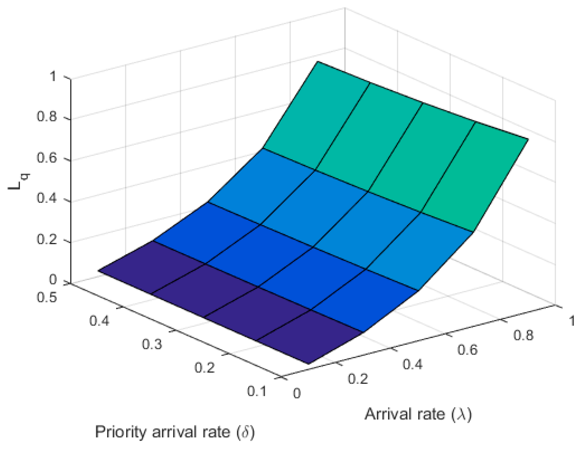
The sensitivity of parameters with respect to different performance indices are explained graphically in Figure 3, Figure 4, Figure 5 and Figure 6. In Figure 3, the surface displays an upward trend as expected for the increasing value of arrival rate of ordinary (λ) and priority (δ) customers against the mean orbit size (Lq).
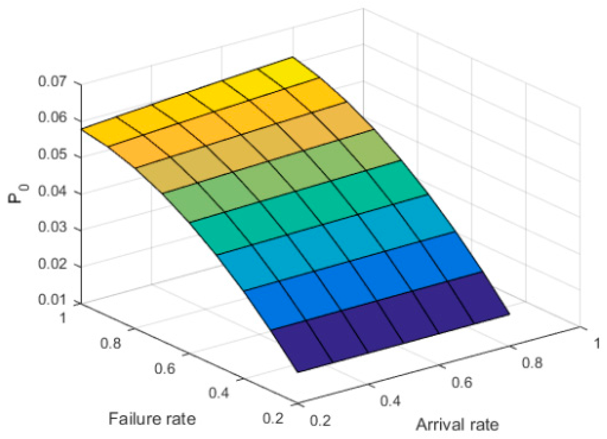
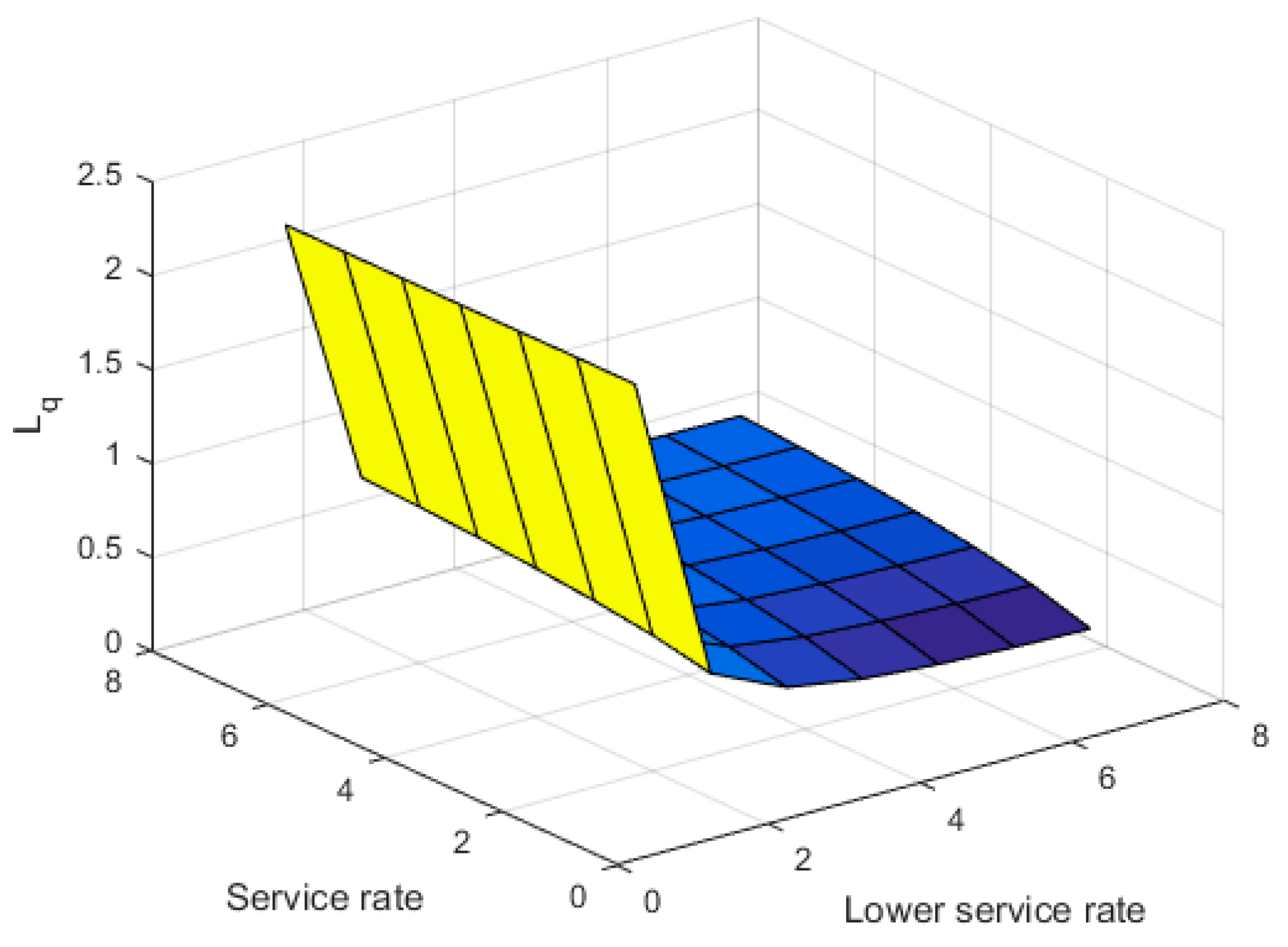
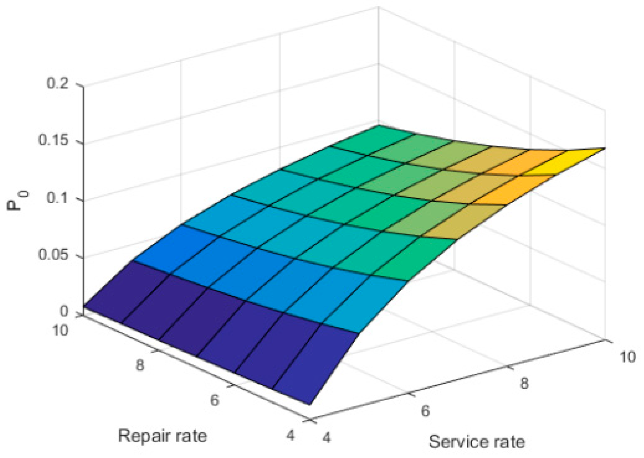
It is found from Figure 4 that P0 decreases with the increasing values of failure rate (α) and ordinary arrival rate (λ). As expected from Figure 5, the mean orbit size (Lq) decreases with the increasing value of the lower service rate (μw) and regular service rate (μ). Figure 6 shows that the idle probability increases with the increasing values of service rate (μ) and repair rate (η).

7. Conclusions

In this investigation, we have studied a preemptive priority retrial queue with disasters under working breakdown services (priority policy for M/G/1/WB). Using the method of the SVT, the PGFs for the system size and its orbit were found. Some important system characteristics like steady state probabilities and the mean system size were obtained. The analytical results were validated with the help of numerical illustrations. The cost optimization was discussed for this model. The novelty of this work is the introduction of a preemptive priority retrial queueing system in the presence of working breakdown services. This proposed model has practical applications in computer processing systems.

Author Contributions

Conceptualization, P.R.; Funding acquisition, S.I.A.; Methodology, P.R.; Software, P.R.; Supervision, S.I.A.; Validation, P.R.; Writing—original draft, P.R.; Both authors are discussed the content & review and edited the manuscript.

Funding

This research received no external funding.

Acknowledgments

The authors would like to thank the anonymous reviewers and editors for their valuable comments and suggestions to improve the quality of this paper.

Conflicts of Interest

The authors declare no conflict of interest.

Appendix A

To prove the sufficient condition of ergodicity, it is very convenient to use Foster’s criterion [25], which states that the chain { Z n ;   n N } is an irreducible and aperiodic Markov chain and is ergodic if there exists a non-negative function f(j), jN and ε> 0, such that the mean drift ψ j = E [ f ( z n + 1 ) f ( z n ) / z n = j ] is finite for all jN and ψ j ε for all jN, except perhaps for a finite value of j. In our case, we consider the function f(j) = j, following which we obtain:
ψ j = { ρ = ( R * ( λ + δ ) + λ R ¯ * ( λ + δ ) ) ( A b S ¯ b * ( α ) + S ( 1 ) ) + δ λ R ¯ * ( λ + δ ) β p ( 1 ) 1 ,   if   j = 0 , ρ = ( R * ( λ + δ ) + λ R ¯ * ( λ + δ ) ) ( A b S ¯ b * ( α ) + S ( 1 ) ) + δ λ R ¯ * ( λ + δ ) β p ( 1 ) R * ( λ + δ ) ,   if   j = 1 , 2
Clearly, the inequality ρ < R * ( λ + δ ) is a sufficient condition for ergodicity.
To prove the necessary condition, as noted in Sennott et al. [26], if the Markov chain { Z n ;   n 1 } satisfies Kaplan’s condition, namely, ψj < ∞ for all j ≥ 0 and there exists j0N such that ψj ≥ 0 for jj0. Notice that, in our case, Kaplan’s condition is satisfied because there is a k such that mij = 0 for j < ik and i > 0, where M = (mij) is the one-step transition matrix of { Z n ;   n N } . Then, ρ R * ( λ + δ ) implies the non-ergodicity of the Markov chain.

References

  1. Artalejo, J.R. Accessible bibliography on retrial queues: Progress in 2000–2009. Math. Comput. Model. 2010, 51, 1071–1081. [Google Scholar] [CrossRef]
  2. Artalejo, J.R.; Corral, A.G. Retrial Queueing Systems; Springer: Berlin, Germany, 2008. [Google Scholar]
  3. Choi, B.D.; Park, K.K. The M/G/1 retrial queue with Bernoulli schedule. Queueing Syst. 1990, 7, 219–228. [Google Scholar] [CrossRef]
  4. Wu, J.; Lian, W. A single-server retrial G-queue with priority and unreliable server under Bernoulli vacation schedule. Comp. Ind. Eng. 2013, 64, 84–93. [Google Scholar] [CrossRef]
  5. Gao, S. A preemptive priority retrial queue with two classes of customers and general retrial times. Oper. Res. 2015, 15, 233–251. [Google Scholar] [CrossRef]
  6. Peng, Y. On the discrete-time Geo/G/1 retrial queueing system with preemptive resume and Bernoulli feedback. Opsearch 2016, 53, 116–130. [Google Scholar] [CrossRef]
  7. Servi, L.D.; Finn, S.G. M/M/1 queues with working vacations. Perform. Eval. 2002, 50, 41–52. [Google Scholar] [CrossRef]
  8. Wu, D.; Takagi, H. M/G/1 queue with multiple working vacations. Perform. Eval. 2006, 63, 654–681. [Google Scholar] [CrossRef] [Green Version]
  9. Van Do, T. M/M/1 retrial queue with working vacations. Acta Inform. 2010, 47, 67–75. [Google Scholar]
  10. Chandrasekaran, V.M.; Indhira, K.; Saravanarajan, M.C.; Rajadurai, P. A survey on working vacation queueing models. Int. J. Pure Appl. Math. 2016, 106, 33–41. [Google Scholar]
  11. Arivudainambi, D.; Godhandaraman, P.; Rajadurai, P. Performance analysis of a single server retrial queue with working vacation. Opsearch 2014, 51, 434–462. [Google Scholar] [CrossRef]
  12. Gao, S.; Wang, J.; Li, W. An M/G/1 retrial queue with general retrial times, working vacations and vacation interruption. Asia-Pac. J. Oper. Res. 2014, 31, 06–31. [Google Scholar] [CrossRef]
  13. Rajadurai, P.; Chandrasekaran, V.M.; Saravanarajan, M.C. Analysis of an unreliable retrial G-queue with working vacations and vacation interruption under Bernoulli schedule. Ain Shams Eng. J. 2018, 9, 56–580. [Google Scholar] [CrossRef]
  14. Gao, S.; Liu, Z. An M/G/1 queue with single working vacation and vacation interruption under Bernoulli schedule. Appl. Math. Model. 2013, 37, 1564–1579. [Google Scholar] [CrossRef]
  15. Zhan, M.; Liu, Q. An M/G/1 G-queue with server breakdown, working vacations and vacation interruption. Opsearch 2015, 52, 256–270. [Google Scholar] [CrossRef]
  16. Kalidass, K.; Ramanath, K. A queue with working breakdowns. Comput. Ind. Eng. 2012, 63, 779–783. [Google Scholar] [CrossRef]
  17. Kim, B.K.; Lee, D.H. The M/G/1 queue with disasters and working breakdowns. Appl. Math. Model. 2014, 38, 1788–1798. [Google Scholar] [CrossRef]
  18. Ma, Z.; Cui, G.; Wang, P.; Hao, Y. M/M/1 vacation queueing system with working breakdowns and variable arrival rate. J. Comput. Inf. Syst. 2015, 11, 1545–1552. [Google Scholar]
  19. Deepa, B.; Kalidass, K. An M/M/1/N Queue with Working Breakdowns and Vacations. Int. J. Pure Appl. Math. 2018, 119, 859–873. [Google Scholar]
  20. Jiang, T.; Liu, L. The GI/M/1 queue in a multi-phase service environment with disasters and working breakdowns. Int. J. Comput. Math. 2017, 94, 707–726. [Google Scholar] [CrossRef]
  21. Liu, Z.; Song, Y. The MX/M/1 queue with working breakdown. Rairo Oper. Res. Rech. Opér. 2014, 48, 399–413. [Google Scholar] [CrossRef]
  22. Rajadurai, P. Sensitivity analysis of an M/G/1 retrial queueing system with disaster under working vacations and working breakdowns. Rairo Oper. Res. 2018, 52, 35–54. [Google Scholar] [CrossRef]
  23. Anandakumar, S.; Ilango, P. PRIN: A Priority-Based Energy Efficient MAC Protocol for Wireless Sensor Networks Varying the Sample Inter-Arrival Time. Wirel. Pers. Commun. 2017, 92, 863–881. [Google Scholar]
  24. Yang, D.Y.; Wu, C.H. Cost-minimization analysis of a working vacation queue with N-policy and server breakdowns. Comp. Ind. Eng. 2015, 82, 151–158. [Google Scholar] [CrossRef]
  25. Pakes, A.G. Some conditions for Ergodicity and recurrence of Markov chains. Oper. Res. 1969, 17, 1058–1061. [Google Scholar] [CrossRef]
  26. Sennott, L.I.; Humblet, P.A.; Tweedi, R.L. Mean drifts and the non Ergodicity of Markov chains. Oper. Res. 1983, 31, 783–789. [Google Scholar] [CrossRef]
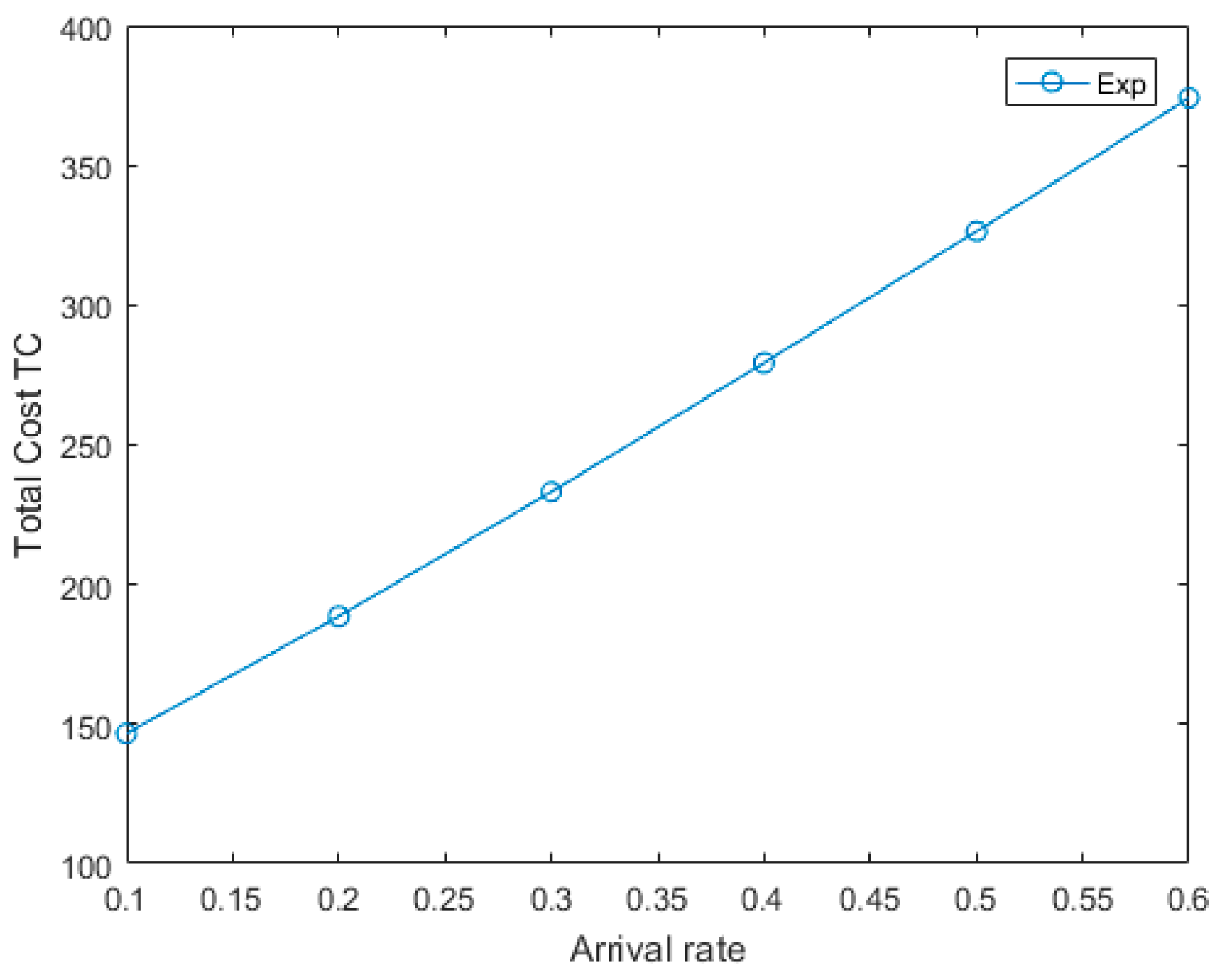
Figure 1. TC versus λ.
Symmetry 11 00419 g001
Figure 2. TC versus α.
Symmetry 11 00419 g002
Figure 3. Lq versus λ and δ.
Symmetry 11 00419 g003
Figure 4. P0 versus λ and α.
Symmetry 11 00419 g004
Figure 5. Lq versus μ and μw.
Symmetry 11 00419 g005
Figure 6. P0 versus μ and η.
Symmetry 11 00419 g006
Table 1. The impact of (Ch, Co) on cost per unit of time (TC) with Cs = $500 and Ca = $90.
(Ch, Co)(5, 60)(20, 60)(15, 60)(5, 75)(5, 100)
TC310.3895311.5580313.1159325.3895350.3895
Table 2. The impact of (Cs, Ca) on TC with Ch = $5 and Co = $60.
(Cs, Ca)(500, 90)(550, 90)(600, 90)(500, 100)(500, 110)
TC310.3895335.3985360.3985323.2147326.3924
Table 3. The impact of retrial rate (θ) on P0, Lq and P.
Retrial Rate (θ)ExpErlangHyp-Exp
P0LqPP0LqPP0LqP
2.000.46734.33450.17320.35075.48420.35380.39864.71280.2318
3.000.52503.85630.11550.47734.07950.22710.47663.94510.1539
4.000.55393.65470.08660.53743.64480.16710.51533.64990.1151
5.000.57123.54340.06930.57243.43370.13210.53853.49370.0920
6.000.58283.47300.05770.59523.30900.10920.55393.39700.0766
Table 4. The impact of priority arrival rate (δ) on P0, Lq and Π1.
Priority Arrival Rate (δ)ExpErlangHyp-Exp
P0LqΠ1P0LqΠ1P0LqΠ1
1.000.72080.08310.00330.42490.24870.02500.68200.16250.0116
2.000.58040.10570.00420.25260.34500.02550.53610.20290.0281
3.000.47600.12630.00430.16140.45220.02230.43410.22110.0446
4.000.39650.14460.00420.10900.56750.01910.35950.22860.0598
5.000.33480.16080.00400.07690.69350.01650.30310.23100.0732