A New GM(1,1) Model Based on Cubic Monotonicity-Preserving Interpolation Spline

Abstract
:1. Introduction
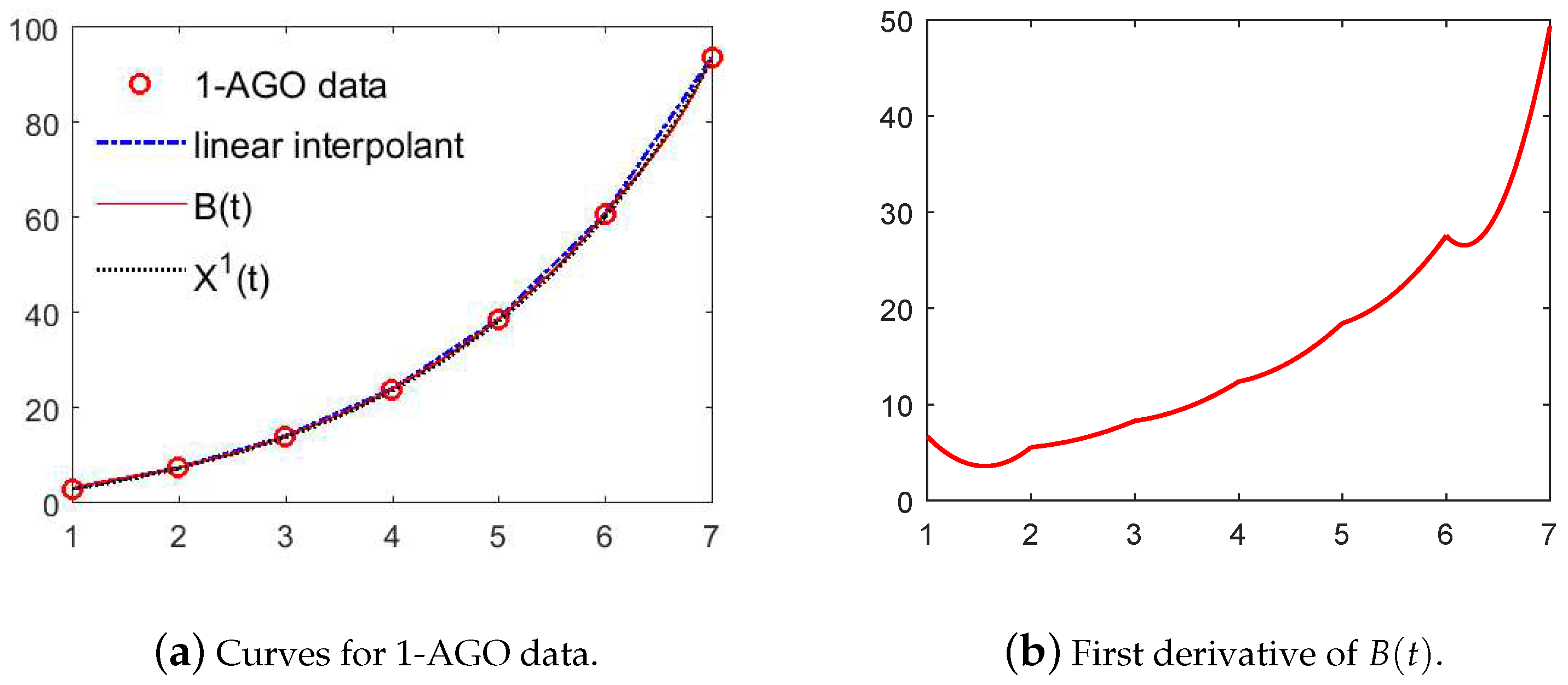
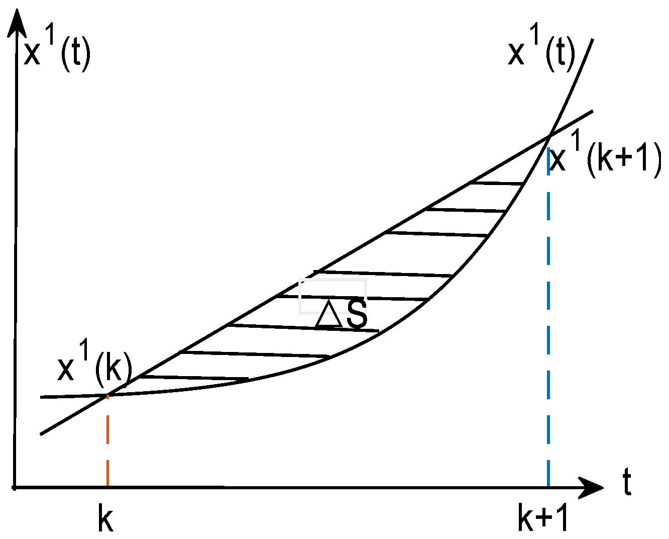
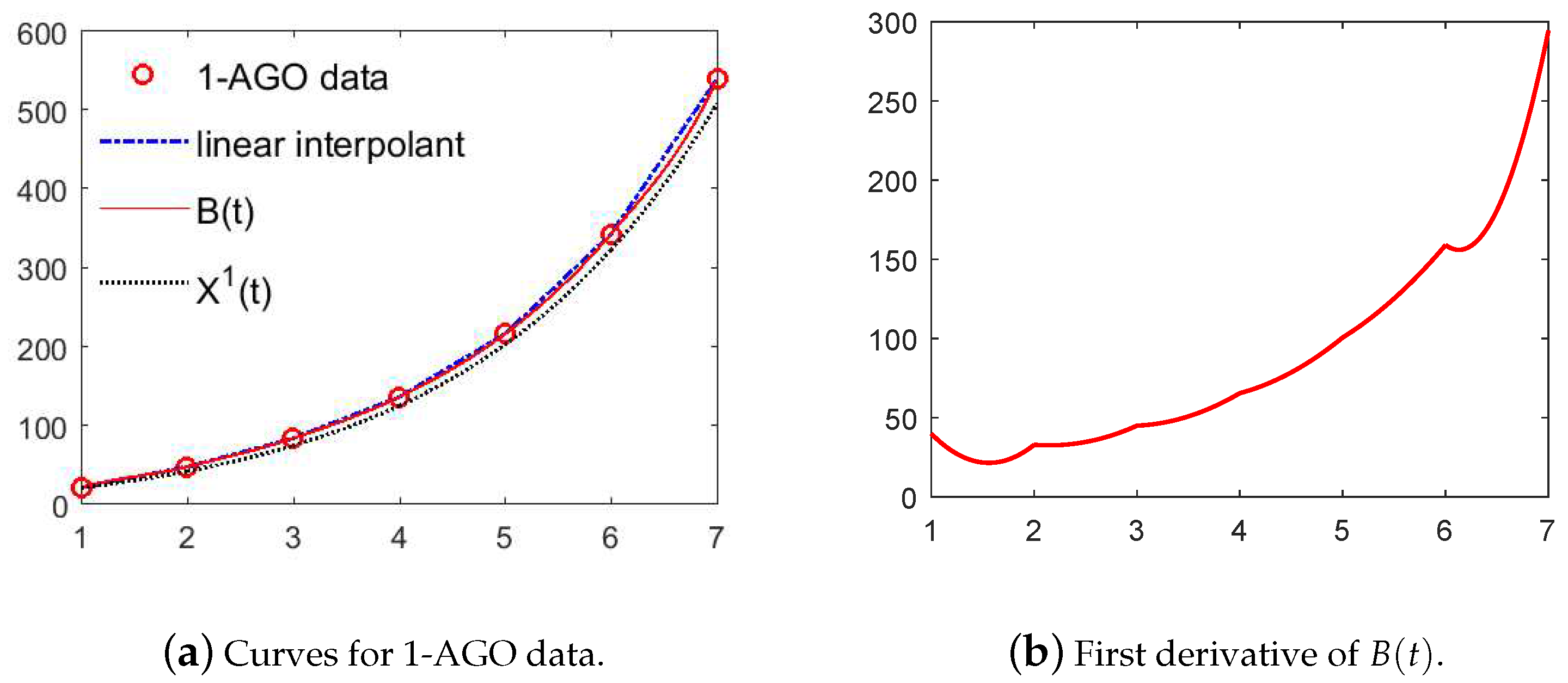
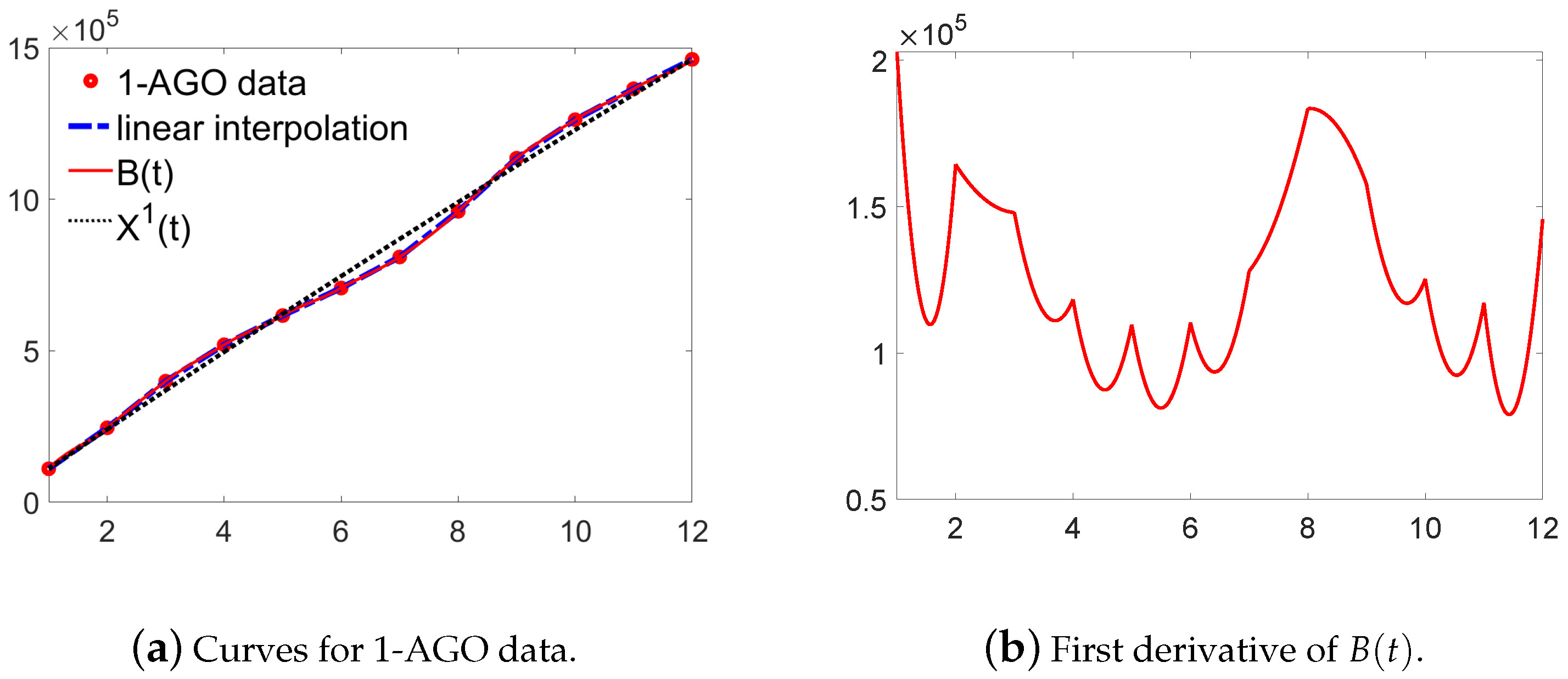
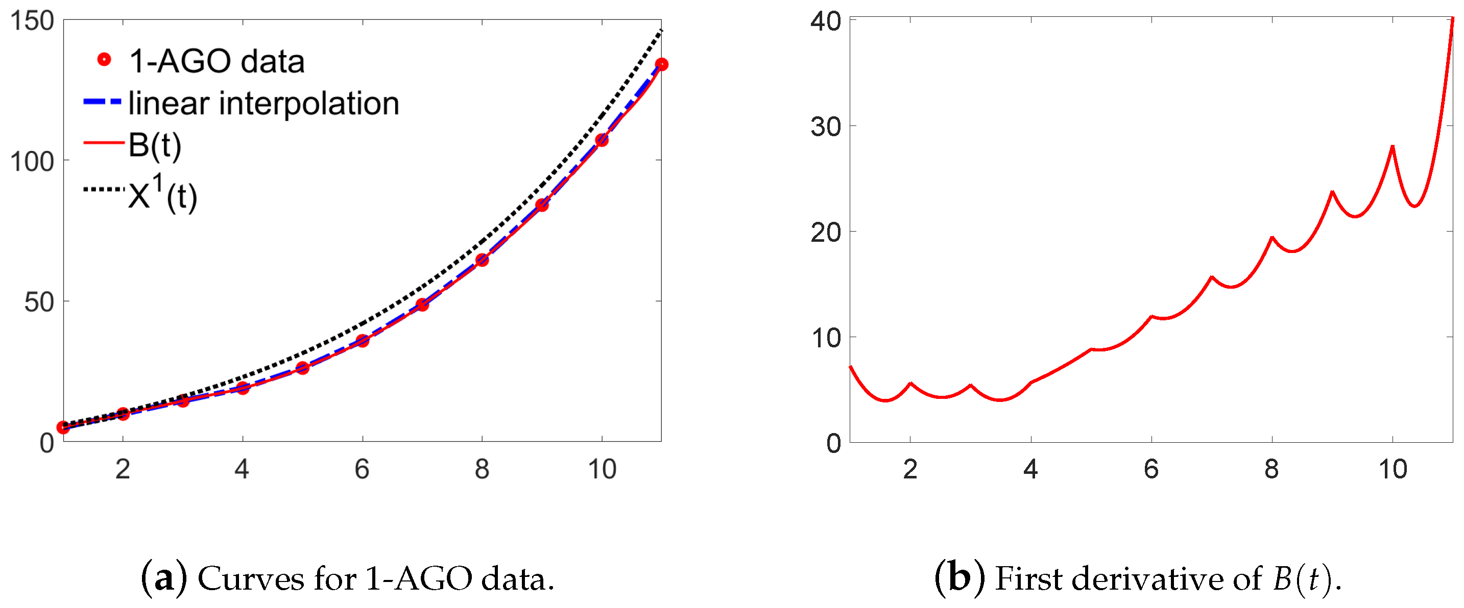
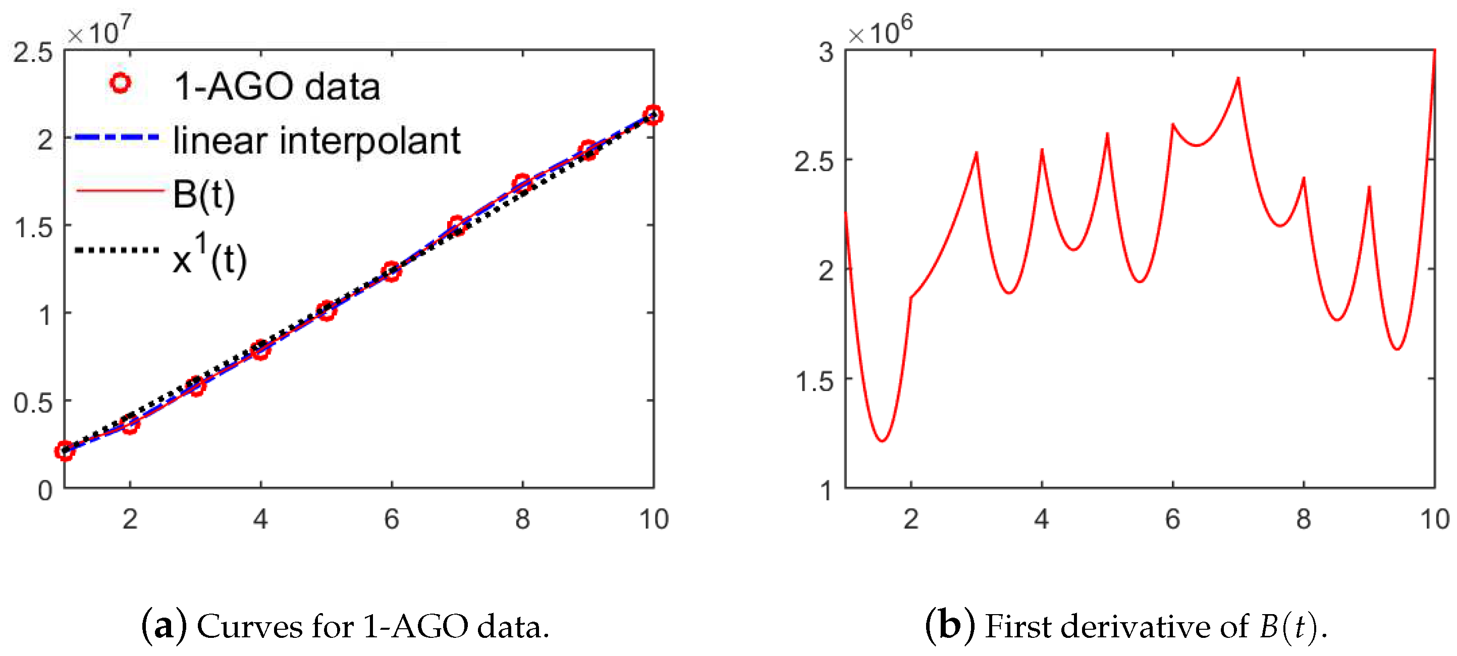
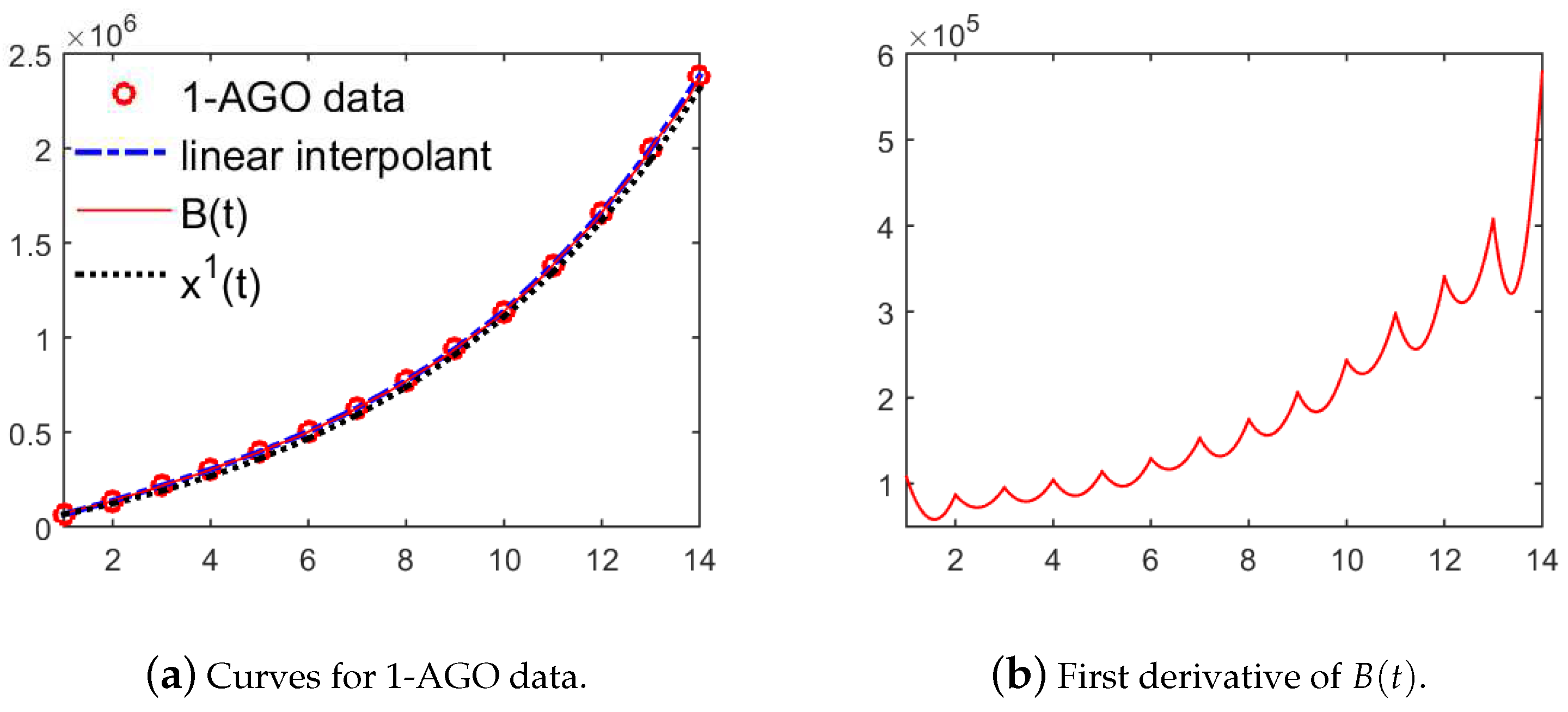
2. Monotonicity-Preserving Piecewise Cubic Interpolation Spline
3. Establish New GM(1,1) Model
4. Conclusions
Author Contributions
Funding
Acknowledgments
Conflicts of Interest
References
- Deng, J. Control problems of Grey system. Syst. Control Lett. 1982, 5, 288–294. [Google Scholar]
- Deng, J. Grey system basic method. In The Basis of Grey Theory; Julong, D., Ed.; Press of Huazhong University of Science and Technology: Wuhan, China, 2002; pp. 210–313. [Google Scholar]
- Tan, G. The structure method and application of background value in grey system GM(1,1) model (I). Syst. Eng. Theory Pract. 2010, 4, 98–103. [Google Scholar]
- Tan, G. The structure method and application of background value in grey system GM(1,1) model (II). Syst. Eng. Theory Pract. 2010, 5, 125–132. [Google Scholar]
- Tan, G. The structure method and application of background value in grey system GM(1,1) model (III). Syst. Eng. Theory Pract. 2010, 6, 70–74. [Google Scholar]
- Li, J.; Dai, W. A new approach of background value building and its application based on data interpolation and Newton-Cotes formula. Syst. Eng. Theory Pract. 2014, 4, 22–126. [Google Scholar]
- Tang, W.; Xiang, C. The improvements of forecasting method in GM(1,1) model based on quadratic interpolation. Chin. J. Manag. Sci. 2006, 14, 109–112. [Google Scholar]
- Wang, X.J.; Yang, S.L.; Ding, J.; Wang, H.J. Dynamic GM(1,1) model based on cubic spline for electricity consumption prediction in smart grid. Chin. Commun. 2010, 7, 83–88. [Google Scholar]
- Wu, L.; Liu, S.; Yao, L.; Yan, S. The effect of sample size on the grey system model. Appl. Math. Model. 2013, 37, 6577–6583. [Google Scholar] [CrossRef]
- Lin, Y.; Ting, Z.; Bingting, Q.; Liu, S. Object multi-attribute differences based grey dynamic clustering method and its application. Oper. Res. Manag. Sci. 2018, 27, 57–63. [Google Scholar]
- Wu, L.; Liu, S.; Fang, Z.; Xu, H. Properties of the GM(1,1) with fractional order accumulation. Appl. Math. Comput. 2015, 252, 287–293. [Google Scholar] [CrossRef]
- Cui, J.; Liu, S.; Zeng, B.; Xie, N. Parameters characteristics of grey Verhulst prediction model under multiple transformation. Control Decis. 2013, 28, 605–608. [Google Scholar]
- Yao, T.X.; Liu, S.F.; Xie, N.M. Study on the properties of new information discrete GM(1,1) model. J. Syst. Eng. 2010, 25, 164–170. [Google Scholar]
- Wang, B.; Xie, N. Unified representation and properties of generalized grey relational analysis models. Syst. Eng. Theory Pract. 2019, 39, 226–235. [Google Scholar]
- Hou, L.; Yang, S.; Wang, X. Mid-term load forecasting based on buffer operator and modified grey model. J. Syst. Simul. 2013, 25, 1–5. [Google Scholar]
- Fan, J.; Gijbels, I. Local Polynomial Modeling and Its Applications; Chapman and Hall: London, UK, 1996. [Google Scholar]
- Bohlin, T. Practical Grey-Box Process Identification: Theory Applications; Springer: Berlin, Germany, 2006. [Google Scholar]
- Wang, Z.; Dang, Y.; Liu, S. An optimal GM(1,1) based on the discrete function with exponential law. Syst. Eng. Theory Pract. 2008, 2, 61–67. [Google Scholar] [CrossRef]
- Tien, T. A new grey prediction model FGM(1,1). Math. Comput. Model. 2009, 49, 1416–1426. [Google Scholar] [CrossRef]
- Wang, Y.; Dang, Y.; Li, Y.; Liu, S. An approach to increase prediction precision of GM(1,1) model based on optimization of the initial condition. Expert Syst. Appl. 2010, 37, 5640–5644. [Google Scholar] [CrossRef]
- Wang, Y.; Liu, Q.; Tang, J.; Cao, W.; Li, X. Optimization approach of background value and initial item for improving prediction precision of GM(1,1) model. J. Syst. Eng. Electron. 2014, 25, 77–82. [Google Scholar] [CrossRef]
- Liu, J.; Xiao, X.; Guo, J.; Mao, S. Error and its upper bound estimation between the solutions of GM(1,1) grey forecasting models. Appl. Math. Comput. 2014, 246, 648–660. [Google Scholar] [CrossRef]
- Chen, P.; Yu, H. Foundation settlement prediction based on a novel NGM model. Math. Probl. Eng. 2014, 2, 1–8. [Google Scholar] [CrossRef]
- He, Z.; Shen, Y.; Li, J.; Wang, Y. Regularized multivariable grey model for stable grey coefficients estimation. Expert Syst. Appl. 2015, 42, 1806–1815. [Google Scholar] [CrossRef]
- Sidorov, D. Integral Dynamical Models: Singularities, Signals and Control; Vol. 87 of World Scientific Series on Nonlinear Science Series A; World Scientific Publ. Pte Ltd.: Singapore, 2015. [Google Scholar]
- Duan, H.; Xiao, X.; Pei, L. Forecasting the short-term traffic flow in the intelligent transportation system based on an inertia nonhomogenous discrete gray model. Complexity 2017, 2017, 1–16. [Google Scholar] [CrossRef]
- Ma, X.; Liu, Z. Application of a novel time-delayed polynomial grey model to predict the natural gas consumption in China. J. Comput. Appl. Math. 2017, 324, 17–24. [Google Scholar] [CrossRef]
- Wer, B.; Xie, N.; Hu, A. Optimal solution for novel grey polynomial prediction model. Appl. Math. Model. 2018, 62, 717–727. [Google Scholar]
- Wang, Z.; Li, Q.; Pei, L. A seasonal GM(1,1) model for forecasting the electricity consumption of the primary economic sectors. Energy 2018, 154, 522–534. [Google Scholar] [CrossRef]
- Zeng, B.; Duan, H.; Bai, Y.; Meng, W. Forecasting the output of shale gas in China using an unbiased grey model and weakening buffer operator. Energy 2018, 151, 238–249. [Google Scholar] [CrossRef]
- Wang, J.; Du, P.; Lu, H.; Yang, W.; Niu, T. An improved grey model optimized by multi-objective ant lion optimization algorithm for annual electricity consumption forecasting. Appl. Soft Comput. 2018, 72, 321–337. [Google Scholar] [CrossRef]


| Classical GM(1,1) | New GM(1,1) | The Model in [20] | ||||
|---|---|---|---|---|---|---|
| Prediction Data | (%) | Prediction Data | (%) | Prediction Data | (%) | |
| 2.9836 | 2.9836 | 0 | 2.9836 | 0 | 2.9836 | 0 |
| 4.4511 | 4.3804 | 1.5816 | 4.3531 | 2.2021 | 4.4561 | 0.1123 |
| 6.6402 | 6.5006 | 2.0903 | 6.5222 | 1.7835 | 6.6132 | 0.4066 |
| 9.9061 | 9.6469 | 2.5994 | 9.7720 | 1.3569 | 9.8146 | 0.9237 |
| 14.7781 | 14.3162 | 3.1039 | 14.6413 | 0.9344 | 14.5657 | 1.4373 |
| 22.0464 | 21.2454 | 3.6069 | 21.9368 | 0.5013 | 21.6168 | 1.9486 |
| 32.8893 | 31.5285 | 4.1065 | 32.8675 | 0.0793 | 32.0812 | 2.4570 |
| (%) | 2.8481 | 1.1429 | 1.2143 | |||
| Classical GM(1,1) | New GM(1,1) | The Model in [21] | ||||
|---|---|---|---|---|---|---|
| Prediction Data | (%) | Prediction Data | (%) | Prediction Data | (%) | |
| 21.1 | 21.1 | 0 | 21.1 | 0 | 21.1000 | 0 |
| 26.6 | 24.4166 | 8.2083 | 24.0779 | 9.4816 | 23.3606 | 12.1782 |
| 36.1 | 35.7198 | 1.0531 | 32.5648 | 9.7928 | 35.7858 | 0.8704 |
| 52.3 | 52.2557 | 0.0847 | 50.3116 | 3.8018 | 54.8198 | 4.8180 |
| 80.1 | 76.4466 | 4.5611 | 77.7300 | 2.9588 | 83.9777 | 4.8411 |
| 126.8 | 111.8361 | 11.8012 | 120.0906 | 5.2913 | 128.6443 | 1.4545 |
| 196.3 | 163.6087 | 16.6537 | 185.5365 | 5.4832 | 197.0684 | 0.3914 |
| (%) | 7.0604 | 6.1349 | 4.0923 | |||
| Classical GM(1,1) | New GM(1,1) | The Model in [7] | ||||
|---|---|---|---|---|---|---|
| Prediction Data | (%) | Prediction Data | (%) | Prediction Data | (%) | |
| 110,852 | 110,852 | 0 | 110,852 | 0 | 110,852 | 0 |
| 135,175 | 117,980 | 12.72 | 130,078 | 3.77 | 127,821 | 5.41 |
| 153,647 | 119,117 | 22.47 | 128,574 | 16.32 | 126,664 | 17.66 |
| 120,296 | 128,264 | 6.62 | 127,087 | 5.64 | 125,830 | 4.68 |
| 96,362 | 121,422 | 26.27 | 125,617 | 30.36 | 124,380 | 29.23 |
| 90,798 | 122,592 | 35.01 | 124,164 | 36.75 | 123,253 | 35.70 |
| 102,591 | 123,773 | 20.65 | 122,728 | 19.63 | 122,137 | 19.11 |
| 150,534 | 124,965 | 16.99 | 121,308 | 19.41 | 121,031 | 19.63 |
| 175,123 | 126,168 | 27.95 | 119,905 | 31.53 | 119,934 | 31.52 |
| 127,148 | 113,383 | 10.83 | 118,518 | 6.79 | 114,848 | 9.76 |
| 102,085 | 128,610 | 25.98 | 117,147 | 14.75 | 117,772 | 15.47 |
| 97,103 | 116,705 | 20.19 | 115,792 | 19.25 | 116,705 | 20.21 |
| (%) | 21.73 | 18.56 | 18.91 | |||
| Classical GM(1,1) | New GM(1,1) | The Model in [9] | ||||
|---|---|---|---|---|---|---|
| Prediction Data | (%) | Prediction Data | (%) | Prediction Data | (%) | |
| 5.08 | 5.08 | 0 | 5.08 | 0 | 5.08 | 0 |
| 4.80 | 3.55 | 26.04 | 4.24 | 11.51 | 3.65 | 23.9 |
| 4.67 | 4.52 | 3.21 | 5.25 | 12.57 | 4.61 | 1.28 |
| 4.50 | 5.76 | 28.00 | 5.51 | 22.44 | 5.84 | 29.78 |
| 7.12 | 7.34 | 3.09 | 8.05 | 13.09 | 7.42 | 4.21 |
| 9.67 | 9.34 | 3.41 | 9.97 | 3.05 | 9.45 | 2.28 |
| 12.80 | 11.90 | 7.03 | 12.33 | 3.64 | 12.04 | 5.94 |
| 15.88 | 15.15 | 4.59 | 15.26 | 3.88 | 15.37 | 3.21 |
| 19.49 | 19.30 | 0.97 | 18.89 | 3.07 | 19.65 | 0.82 |
| 23.07 | 24.57 | 6.50 | 23.38 | 1.34 | 24.57 | 8.92 |
| 26.86 | 31.29 | 16.49 | 28.93 | 7.72 | 31.29 | 19.73 |
| (%) | 9.03 | 7.48 | 8.29 | |||
| Classical GM(1,1) | New GM(1,1) | The Model in [11] | ||||
|---|---|---|---|---|---|---|
| Prediction Data | (%) | Prediction Data | (%) | Prediction Data | (%) | |
| 1610.71 | 1610.71 | 0 | 1610.71 | 0 | 1610.71 | 0 |
| 1245.28 | 1363.91 | 9.524 | 1365.22 | 9.632 | 1342.76 | 7.833 |
| 1347.71 | 1274.95 | 5.402 | 1275.75 | 5.340 | 1280.32 | 5.004 |
| 1382.45 | 1191.79 | 13.795 | 1192.14 | 13.766 | 1204.58 | 12.872 |
| 1018.45 | 1114.06 | 9.381 | 1114.01 | 9.383 | 1122.64 | 10.203 |
| 1014.96 | 1041.39 | 2.597 | 1041.00 | 2.566 | 1040.18 | 2.476 |
| 949.46 | 973.47 | 2.519 | 972.78 | 2.456 | 960.34 | 1.147 |
| (%) | 6.174 | 6.163 | 5.648 | |||
| Classical GM(1,1) | New GM(1,1) | |||
|---|---|---|---|---|
| Prediction Data | (%) | Prediction Data | (%) | |
| 64,832.05 | 64,832.05 | 0 | 64,832.05 | 0 |
| 71,847.09 | 57,476.77 | 20.001 | 57,308.50 | 20.235 |
| 78,646.30 | 67,165.21 | 14.598 | 67,022.83 | 14.779 |
| 86,293.10 | 78,486.76 | 9.046 | 78,383.83 | 9.166 |
| 93,887.95 | 91,716.70 | 2.312 | 91,670.62 | 2.362 |
| 105,557.09 | 107,176.71 | 1.534 | 107,209.65 | 1.566 |
| 125,761.85 | 125,242.71 | 0.413 | 125,382.70 | 0.301 |
| 143,143.63 | 146,353.96 | 2.243 | 146,636.24 | 2.440 |
| 168,850.20 | 171,023.78 | 1.287 | 171,492.46 | 1.565 |
| 198,739.27 | 199,852.01 | 0.560 | 200,562.04 | 0.917 |
| 245,352.80 | 233,539.60 | 4.815 | 234,559.18 | 4.400 |
| 278,541.09 | 272,905.57 | 2.023 | 274,319.16 | 1.516 |
| 334,839.41 | 318,907.39 | 4.758 | 320,818.83 | 4.187 |
| 386,086.72 | 372,663.28 | 3.477 | 375,200.63 | 2.820 |
| (%) | 4.791 | 4.732 | ||
© 2019 by the authors. Licensee MDPI, Basel, Switzerland. This article is an open access article distributed under the terms and conditions of the Creative Commons Attribution (CC BY) license (http://creativecommons.org/licenses/by/4.0/).
Share and Cite
Zhu, Y.; Jian, Z.; Du, Y.; Chen, W.; Fang, J. A New GM(1,1) Model Based on Cubic Monotonicity-Preserving Interpolation Spline. Symmetry 2019, 11, 420. https://doi.org/10.3390/sym11030420
Zhu Y, Jian Z, Du Y, Chen W, Fang J. A New GM(1,1) Model Based on Cubic Monotonicity-Preserving Interpolation Spline. Symmetry. 2019; 11(3):420. https://doi.org/10.3390/sym11030420
Chicago/Turabian StyleZhu, Yuanpeng, Zehua Jian, Yurui Du, Wenqing Chen, and Jiwei Fang. 2019. "A New GM(1,1) Model Based on Cubic Monotonicity-Preserving Interpolation Spline" Symmetry 11, no. 3: 420. https://doi.org/10.3390/sym11030420
APA StyleZhu, Y., Jian, Z., Du, Y., Chen, W., & Fang, J. (2019). A New GM(1,1) Model Based on Cubic Monotonicity-Preserving Interpolation Spline. Symmetry, 11(3), 420. https://doi.org/10.3390/sym11030420